Multilayer Adsorption of Polyatomic Species on Homogeneous and Heterogeneous Surfaces

Abstract

In this work we study the multilayer adsorption of polyatomic species on homogeneous and heterogeneous bivariate surfaces. A new approximate analytic isotherm is obtained and validated by comparing with Monte Carlo simulation. Then, we use the well-known Brunauer-Emmet-Teller’s (BET) approach to analyze these isotherms and to estimate the monolayer volume, $v_{\mathrm{m}}$. The results show that the value of the $v_{\mathrm{m}}$ obtained in this way depends strongly on adsorbate size and surface topography. In all cases, we find that the use of the BET equation leads to an underestimate of the true monolayer capacity.

1 Introduction

The theoretical description of multilayer adsorption is a long-standing important problem in surface science that does not have a general solution. [1, 2] Mainly this is due to the fact that the structure of the different layers differs from that in contact with the solid surface (first layer). At high coverage (multilayer region), it is expected that the adsorption process is well described by the slab theory of Frenkel, Halsey and Hill. [3, 4, 5] In this approach it is assumed that the higher layers retain the structure of the bulk liquid, and only its free energy changes gradually as one goes away from the solid surface. On the other hand, at low coverage, it is more appropriate to use the Brunauer-Emmet-Teller’s (BET) isotherm, [6] where the crystal-like structure of the surface is considered. In the BET theory it is assumed that the molecules are localized in sites and that the adsorption in the first layer is different from the remaining ones.

The BET equation is one of the most widely used isotherms. The approach discards such things as the polyatomic character of the adsorbate, the interaction between the admolecules and the surface heterogeneities. Then, with the purpose of including a more complex situation, numerous generalizations of the BET theory have been proposed. [2, 7] Nevertheless, the simplicity of the BET isotherm has made it very popular for practical purposes. In fact, by fitting an experimental isotherm with the BET equation, in many cases it is possible to predict the monolayer volume (or monolayer capacity) of the solid surface with an error not bigger than the $20\%$. [1] This surprising result is attributed to compensation effects arisen as consequence of having carried out many approximations. [1]

By means of numerical experiments, Walker and Zettlemoyer [8] have shown that the conventional BET theory predicts a monolayer volume smaller than the real value, when heterogeneous adsorption isotherms are analyzed. A similar result was obtained by Cortés and Araya, [9] when considering a Gaussian distribution of adsorption energies. The authors showed that the estimated values of the monolayer volume from the BET equation diminishes with increasing degree of surface heterogeneity (the width of the distribution of adsorption energies).

More recently, Nikitas [10] has arrived to similar conclusions by considering both, surface heterogeneity and polyatomic character of the adsorbate. In ref [10], by using an extension of the Flory-Huggins polymer solution theory, [7] the multilayer adsorption of polyatomic species was studied over a random heterogeneous surface. By particular cases analysis, the author concludes that one can obtain an underestimation of the true monolayer capacity of the order of $25\%$, when the adsorbate occupies more than one lattice site. This underestimation is bigger, if an heterogeneous surface is considered.

In this work, we study how the monolayer volume predicted by BET equation differs from its real value when considering both the adsorbate size and the surface topography, i. e. the space distribution of the adsorption energies over the solid surface. In particular, we consider the multilayer adsorption of polyatomic species on one-dimensional (1D) and two-dimensional (2D) homogeneous and heterogeneous bivariate surfaces. In each case, approximate analytic isotherms are built and validated by comparing with Monte Carlo simulation. Then, we estimate the monolayer volume, by analyzing these isotherms with the conventional BET theory.

The paper is structured as follows. In section 2, we present the lattice-gas model. Next, in sections 3 and 4, the multilayer adsorption isotherms for homogeneous and heterogeneous surfaces are obtained. The dependence of the monolayer volume on the surface topography and the adsorbate size is presented in section 5. Finally, conclusions are drawn in section 6.

2 The Lattice-Gas Model

A simple lattice-gas model to describe the multilayer adsorption of polyatomic molecules on homogeneous surface has been recently proposed. [11, 12] The surface is modeled by a regular lattice of $M$ sites, all with the same adsorption energy $\varepsilon$, and the adsorbate is represented by $k$-mers (linear particles that have $k$ identical units). A $k$-mer adsorbed on the surface occupies $k$ sites of the lattice with an energy $k\varepsilon$ and can arrange in many configurations. This property is called adsorption with multisite occupancy. On the other hand, for higher layers, the adsorption of a $k$-mer is exactly onto an already absorbed one, with an adsorption energy of $kU$. Thus, the monolayer structure reproduces in the remaining layers. This phenomenon is called pseudomorphism and, for example, is observed experimentally in the adsorption of straight chain saturated hydrocarbon molecules. [13] Finally, following the spirit of the BET theory, no lateral interactions are considered and only interactions among the layers are introduced. Figure 1 in ref [11] shows a snapshot representing this lattice-gas model.

We modify the model to consider the adsorption on a heterogeneous substrate: now the adsorption energy $\varepsilon_{i}$ depends on each site $i$ of the surface. Then, the Hamiltonian of the system is

$$H=\left(N-N_{\mathrm{m}}\right)kU+\sum_{i=1}^{M}\sigma_{i}\varepsilon_{i},$$ (1)

where $N$ is the total number of $k$-mers, $\sigma_{i}$ the occupation variable which can take the values 0 if the corresponding site is empty or 1 if the site is occupied, and $N_{\mathrm{m}}$ is the number of $k$-mers on the surface (monolayer),

$$N_{\mathrm{m}}=\frac{1}{k}\sum_{i=1}^{M}\sigma_{i}.$$ (2)

The Hamiltonian in eq (1) can be rewritten as

$$H=NkU+\sum_{i=1}^{M}\sigma_{i}\left(\varepsilon_{i}-U\right).$$ (3)

In the following sections, we will look for analytic solutions of the model in 1D and 2D, for homogeneous and heterogeneous surfaces.

3 Multilayer Adsorption on Homogeneous Surfaces

For the previous model, a simple analytic expression of the multilayer adsorption isotherm can be obtained in few particular cases. If the surface is homogeneous ($\varepsilon_{i}=\varepsilon$ for all $i$) and $k=1$, it is easy to demonstrate [1, 2, 11] that

$$\theta=\frac{1}{\left(1-p/p_{0}\right)}\frac{cp/p_{0}}{\left[1+\left(c-1\right)p/p_{0}\right]}.$$ (4)

Here, $\theta=kN/M$ is the total coverage, $p$ is the pressure, $p_{0}$ is the saturation pressure of the bulk liquid and $c$ is a constant defined as

$$c=\exp\left[-\beta k\left(\varepsilon-U\right)\right],$$ (5)

where $\beta=1/k_{B}T$ is the inverse temperature (being $k_{B}$ the Boltzmann constant and $T$ the absolute temperature). eq (4) is the well-known BET isotherm [6] and can be applied to systems in any dimension.

In the case of $k=2$, it is only possible to obtain an exact solution in 1D [11]

$$\theta=\frac{1}{\left(1-p/p_{0}\right)}\left\{1-\left[\frac{1-p/p_{0}}{1+\left(4c-1\right)p/p_{0}}\right]^{1/2}\right\}.$$ (6)

Equation (6) is the exact dimer isotherm for the multilayer adsorption on 1D homogeneous surface. As it has been previously shown, [11] the values of the monolayer volume predicted by eqs (4) and (6) are different: if a dimer isotherm is analyzed, the value of the monolayer capacity arising from using BET characterization is smaller than the real one.

In general, the multilayer isotherm corresponding to the model of eq (3) cannot be expressed by one equation only. To describe the isotherm, it is necessary to give two functions. [10, 12] Let us assume that an analytical expression of the monolayer adsorption isotherm is known, $\exp\left(\mu\beta\right)=\lambda$, being $\mu$ the chemical potential and $\lambda$ (the fugacity) a function of the monolayer coverage $\theta_{\mathrm{m}}=kN_{\mathrm{m}}/M$. Then, the following equations can be deduced [12]:

$$\frac{p}{p_{0}}=\frac{\lambda\left(\theta_{\mathrm{m}}\right)}{c+\lambda\left(\theta_{\mathrm{m}}\right)}$$ (7)

and

$$\theta=\frac{\theta_{\mathrm{m}}}{\left(1+p/p_{0}\right)}.$$ (8)

Equations (7) and (8) constitute the multilayer adsorption isotherm. By using the surface coverage ($0\leq\theta_{\mathrm{m}}\leq 1$) as a parameter, we can calculate the relative pressure from eq (7). Then, the values of $\theta_{\mathrm{m}}$ and $p/p_{0}$ are introduced in eq (8) and the total coverage is obtained.

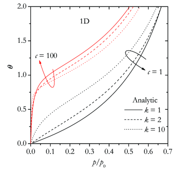
Figure 1: Exact 1D isotherms for $k=1$, 2 and 10, and two values of $c$ as indicated.

Following the previous scheme, it is possible to obtain the exact multilayer isotherm for $k$-mers in 1D homogeneous surfaces. [12] We start from the exact monolayer isotherm [14]

$$\lambda=\frac{\theta_{\mathrm{m}}\left[1-\frac{\left(k-1\right)}{k}\theta_{\mathrm{m}}\right]^{k-1}}{k\left(1-\theta_{\mathrm{m}}\right)^{k}}.$$ (9)

Then, eq (7) can be written as

$$\frac{p}{p_{0}}=\frac{\theta_{\mathrm{m}}\left[1-\frac{\left(k-1\right)}{k}\theta_{\mathrm{m}}\right]^{k-1}}{kc\left(1-\theta_{\mathrm{m}}\right)^{k}+\theta_{\mathrm{m}}\left[1-\frac{\left(k-1\right)}{k}\theta_{\mathrm{m}}\right]^{k-1}}.$$ (10)

Equations (10) and (8) represent the exact solution of the 1D model. In particular, for $k=1$ and $k=2$, it is possible to solve these equations to obtain single expressions of the multilayer isotherms, eqs (4) and (6), respectively. Figure 1 shows the exact 1D isotherms for $k=1$, 2 and 10, and two values of $c$.

Also, the previous scheme can be used to obtain an accurate approximation for multilayer adsorption on 2D substrates accounting multisite occupancy. In this case, we use the semi-empirical (SE) monolayer adsorption isotherm [15, 16]

$$\lambda=\frac{2\theta_{\mathrm{m}}\left[1-\frac{\left(k-1\right)}{k}\theta_{\mathrm{m}}\right]^{\left(k-1\right)\theta_{\mathrm{m}}}\left[1-\frac{2\left(k-1\right)}{\gamma k}\theta_{\mathrm{m}}\right]^{\left(k-1\right)\left(1-\theta_{\mathrm{m}}\right)}}{\gamma k\left(1-\theta_{\mathrm{m}}\right)^{k}},$$ (11)

where $\gamma$ is the connectivity of the lattice. It has been shown that eq (11) is a very good approximation for representing multisite-occupancy adsorption in the monolayer regime. [15, 16] Then, by using eqs (7) and (11) we obtain

$$\frac{p}{p_{0}}=\frac{2\theta_{\mathrm{m}}\left[1-\frac{\left(k-1\right)}{k}\theta_{\mathrm{m}}\right]^{\left(k-1\right)\theta_{\mathrm{m}}}\left[1-\frac{2\left(k-1\right)}{\gamma k}\theta_{\mathrm{m}}\right]^{\left(k-1\right)\left(1-\theta_{\mathrm{m}}\right)}}{\gamma kc\left(1-\theta_{\mathrm{m}}\right)^{k}+2\theta_{\mathrm{m}}\left[1-\frac{\left(k-1\right)}{k}\theta_{\mathrm{m}}\right]^{\left(k-1\right)\theta_{\mathrm{m}}}\left[1-\frac{2\left(k-1\right)}{\gamma k}\theta_{\mathrm{m}}\right]^{\left(k-1\right)\left(1-\theta_{\mathrm{m}}\right)}}.$$ (12)

Note that, for $\gamma=2$, the SE isotherm is identical to the eq (9). Therefore, eqs (8) and (12) represent the general solution of the problem of multilayer adsorption in homogeneous surfaces with multisite occupancy: for $\gamma=2$ (1D) this isotherm is exact, but is approximate for $\gamma>2$. In addition, in any dimension, the exact isotherm for $k=1$ (BET equation) can also be obtained from eqs (8) and (12), but always with $\gamma=2$ (these equations with $k=1$ and $\gamma>2$ are erroneous, because do not provide the BET isotherm).

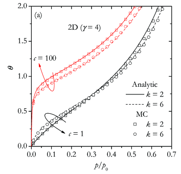
Figure 2: Comparison between analytic and simulated adsorption isotherms for 2D lattices and two different values of $c$ as indicated. (a) $k=2$ and 6, (b) $k=10$. In all cases, we have used $t=10^{5}$ MCSs.

In order to test the 2D approximation, we have compared the analytic multilayer isotherm with results of Monte Carlo (MC) simulation. The algorithm used is described in ref [12]. Here, the equilibrium state is reproduced after discarding a number $t$ of MC steps (MCSs). Then, the mean value of the total coverage is obtained as,

$$\theta=\frac{k\langle N\rangle}{M},$$ (13)

where the average $\langle N\rangle$ is calculated over another $t$ successive MCSs (the total number of MCSs is $2t$). The computational simulations were developed for a square lattice ($\gamma=4$) of linear size $L$ ($M=L\times L$). For each value of $k$, we choose $L=20k$. For these lattice sizes (proportional to $k$), we have verified that finite-size effects are negligible.

Figure 2a shows a comparison between the analytic isotherm [given by eqs (8) and (12)] and the MC results, for $k=2$ and 6 and two values of $c$. As we can see, the agreement is very good for the parameters used in the figure. On the other hand, the accuracy of the analytic isotherm diminishes as $k$ increases. Figure 2b shows this effect for $k=10$. Also, in this figure, we can appreciate that the difference between the analytic and the numerical isotherm diminishes as $c$ is increased.

4 Multilayer Adsorption on Heterogeneous Surfaces

In the previous section, we have obtained the multilayer isotherm from the monolayer isotherm. It is possible demonstrate that in general, the formalism allows to establish this connection only if $(1)$ pseudomorphism is present and $(2)$ no lateral interactions between the molecules in the multilayer regime are considered. In fact, eqs (7) and (8) still hold if the particles in the monolayer interact among them and with the solid surface. Although we could use this formalism to determine the multilayer adsorption isotherm for a given surface heterogeneity (for which it would be necessary to have an appropriate monolayer isotherm), we have chosen to use a different strategy.

We start here from the integral representation of the adsorption multilayer isotherm [2]

$$\theta=\int\chi(\varepsilon)\theta_{\mathrm{loc}}(\varepsilon)d\varepsilon,$$ (14)

where $\theta_{\mathrm{loc}}(\varepsilon)$ represents the local adsorption multilayer isotherm corresponding to an adsorptive site of energy $\varepsilon$ and $\chi(\varepsilon)$ is the adsorptive energy distribution which characterizes the surface heterogeneity (as before, the total and the local coverage depend on $p$ and $T$).

It should be noticed that eq (14) is strictly and generally valid only for noninteracting monomers ($k=1$), which is a quite unrealistic case. If adsorbed particles occupy more than one site (multisite occupancy) or interact with each other, then the local coverage at a point with a given adsorptive energy depends on the local coverage on neighbor points with different adsorptive energies and, in general, eq (14) should be replaced by a much more complex expression. [17, 18]

Nevertheless, in some situations eq (14) represents a good approximation of the adsorption isotherm (see below). For a lattice-gas model of $k$-mers, we can generalize this equation as

$$\theta=\sum_{s}\theta_{\mathrm{loc}}(E_{s}).$$ (15)

In the last equation, the sum extends over all possible configurations of a single $k$-mer in an empty lattice, and $E_{s}$ is the adsorption energy of each one of them. Note that the values of $E_{s}$ depend, among other things, on the energy distribution $\chi(\varepsilon)$, the surface topography and the number $k$.

In following sections, we will study the multilayer adsorption on 1D and 2D heterogeneous surfaces. As local isotherm, we will use eqs (8) and (12). Then, we will compare the multilayer adsorption isotherm obtained by using eq (15) and the calculated with MC simulation.

4.1 Adsorption on 1D Heterogeneous Surfaces

As we said in the introduction, the heterogeneity is modeled by two kinds of sites (bivariate surface): strong sites with adsorption energy $\varepsilon_{1}$ and weak sites with adsorption energy $\varepsilon_{2}$ ($\varepsilon_{1}<\varepsilon_{2}$). In 1D, where the surface is represented by a chain of sites with periodic boundary conditions, these sites form patches of size $l$ $(l=1,2,3,\cdots)$, which are spatially distributed (topography) in a deterministic alternate way.

The number of possible configurations of a single $k$-mer in an empty lattice is $M$. However, due to periodicity, eq (15) has only $2l$ terms (with many of them having the same adsorption energy). Then, the multilayer isotherm is approximated as

$$\theta=\frac{1}{2l}\sum_{i=1}^{2l}\theta_{\mathrm{loc}}\left(c_{i}\right).$$ (16)

Each term corresponds to an effective value of $c$ given by

$$c_{i}=\exp\left[-\beta\left(E_{i}-kU\right)\right],$$ (17)

where $E_{i}$ is the adsorption energy. This value of $c_{i}$ can also be expressed as function of $c_{1}$ and $c_{2}$, the values of $c$ for homogeneous surfaces given by eq (5) and whose adsorption energies are $\varepsilon_{1}$ and $\varepsilon_{2}$, respectively. If the $i$-th term in eq (16) corresponds to a $k$-mer with $k_{1}$ units located over strong sites and $k_{2}$ units located over weak sites, then the adsorption energy is $E_{i}=k_{1}\varepsilon_{1}+k_{2}\varepsilon_{2}$, and

$$c_{i}=\left(c_{1}^{k_{1}}c_{2}^{k_{2}}\right)^{1/k}.$$ (18)

As mentioned previously, we use eqs (8) and (12) with $\gamma=2$ as local isotherm. Note that eq (16) is a sum of local isotherms with different values of $c$, but at the same relative pressure. Then, in most of the cases it is necessary to be careful: although, for each local isotherm the surface coverage should be used as a parameter, it is not possible to use this as common parameter. In fact, eq (7) shows that for a fixed value of $p/p_{0}$, the surface coverage depends on $c$, $\theta_{\mathrm{m}}(c_{i})$.

Now, we analyze two simple cases. On one hand, eq (16) is exact for $k=1$ and can be obtained as the semisum of two BET isotherms,

$$\theta=\frac{p/p_{0}}{2\left(1-p/p_{0}\right)}\left\{\frac{c_{1}}{\left[1+\left(c_{1}-1\right)p/p_{0}\right]}+\frac{c_{2}}{\left[1+\left(c_{2}-1\right)p/p_{0}\right]}\right\}.$$ (19)

In this case, eq (19) does not depend on $l$ and, consequently, the multilayer adsorption isotherm is the same for all topography.

On the other hand, eq (16) has three different terms for $k=2$, being each one of them a dimer isotherm eq (6) with a particular value of $c$. Thus, for $k=2$, the multilayer adsorption isotherm is

$$\theta = \left(\frac{l-1}{2l}\right)\frac{1}{\left(1-p/p_{0}\right)}\left\{1-\left[\frac{1-p/p_{0}}{1+\left(4c_{1}-1\right)p/p_{0}}\right]^{1/2}\right\}+$$ (20)

$$+ \left(\frac{1}{l}\right)\frac{1}{\left(1-p/p_{0}\right)}\left\{1-\left[\frac{1-p/p_{0}}{1+\left(4\sqrt{c_{1}c_{2}}-1\right)p/p_{0}}\right]^{1/2}\right\}+$$

$$+ \left(\frac{l-1}{2l}\right)\frac{1}{\left(1-p/p_{0}\right)}\left\{1-\left[\frac{1-p/p_{0}}{1+\left(4c_{2}-1\right)p/p_{0}}\right]^{1/2}\right\}.$$

The first [third] term in the RHS of eq (20) represents the adsorption within a strong [weak] patch, on a pair of sites (1,1) [(2,2)], with $c_{1}$ [$c_{2}$]. There are $(l-1)$ configurations of this for each patch. The remaining term of eq (20) corresponds to a dimer isotherm with adsorption energy $E=\varepsilon_{1}+\varepsilon_{2}$ ($c=\sqrt{c_{1}c_{2}}$). There are only two configurations with this energy for pairs of sites (1,2) or (2,1). Contrary to eq (19), eq (20) depends on $l$ and the dimer isotherm sees the topography.

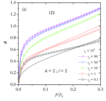
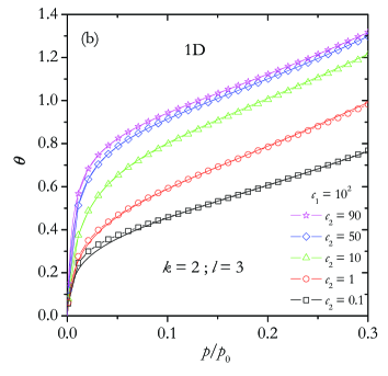
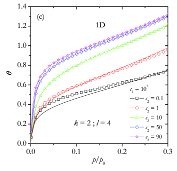
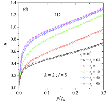
Figure 3: Comparison between approximate analytic and MC isotherms for dimers and different 1D heterogeneous surfaces: (a) $l=2$, (b) $l=3$, (c) $l=4$ and (d) $l=5$. In all cases we have used lattices of size $L=1200$ and $t=10^{5}$ MCSs.

For $l=1$, the adsorption energy of a dimer is $E=\varepsilon_{1}+\varepsilon_{2}$ for all configuration and, consequently, eq (20) is exact. In general, for $l>1$ and $c_{1}\neq c_{2}$, this equation is approximate. Then, to determine the range of validity of this equation, we compare the analytic isotherm with MC results. Figure 3a shows the dimer isotherm for patches of size $l=2$, $c_{1}=10^{2}$ and different values of $c_{2}$. As we can see, for $c_{2}\geq 10$ the analytic isotherms agree very well with the MC data. However, for smaller values of $c_{2}$, the differences between theoretical and numerical data begin to be significant. This happens because eq (20) has been built assuming that the three different pairs of sites are filled simultaneously and independently. However, for $c_{1}\gg c_{2}$, the real process occurs in 3 stages: $(i)$ the pairs of sites (1,1) are covered; $(ii)$ the pairs (2,2) begin to be filled and $(iii)$ the multilayer is formed. Note that in the first stage all the pair of sites (1,2) and (2,1) are removed. For this regime, a better approximation can be obtained by a semisum of two isotherms with $c_{1}$ y $c_{2}$.

When $l=3$, Figure 3b, the agreement between the analytic isotherms and the MC data is very good for all values of $c_{2}$. In this case, for $c_{1}\gg c_{2}$ the first stage does not eliminate all the pairs of sites (1,2) and (2,1), because each dimer occupies only two sites in the strong patches. For this reason, the range of validity of eq (20) is wider than in the previous case. Now, if $l=4$ or $l=5$, we see in Figures 3c and d that the behaviors are similar to those observed for $l=2$ or $l=3$, respectively. In general, for even $l$, the first stage eliminates almost completely the pairs of sites (1,2) and (2,1), while this does not happen for odd $l$. Finally, when $l\to\infty$, the fraction of pair (1,2) and (2,1) goes to zero and eq (20) is exact. This limit corresponds to the called large patches topography (LPT), where the surface is assumed to be a collection of homogeneous patches, large enough to neglect border effects between neighbor patches with different adsorption energies.

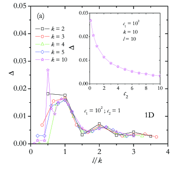
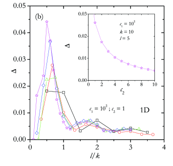
Figure 4: Function $\Delta$ vs $l/k$ for the adsorption in a 1D heterogeneous surface with $c_{1}=10^{2}$, $c_{2}=1$ and different values of $k$ as indicated. (a) Function $\Delta$ calculated from eq (16). The inset shows the dependence of $\Delta$ on $c_{2}$ for $k=10$ and $l=10$. b) Function $\Delta$ calculated from eq (23). The inset shows the dependence of $\Delta$ on $c_{2}$ for $k=10$ and $l=5$.

In general, if $k\gg l$ (with $k>1$), the multilayer adsorption isotherm can be represented by a single homogeneous isotherm

$$\theta=\theta_{\mathrm{loc}}\left(\sqrt{c_{1}c_{2}}\right).$$ (21)

On the other hand, for a LPT where $k\ll l$, the isotherm is

$$\theta=\frac{1}{2}\theta_{\mathrm{loc}}\left(c_{1}\right)+\frac{1}{2}\theta_{\mathrm{loc}}\left(c_{2}\right).$$ (22)

The details of the topography are relevant only when $k\sim l$. In this case, all terms in eq (16) are important. Nevertheless, it is also interesting to obtain a simpler expression of the multilayer isotherm given by

$$\theta=\left(\frac{l-1}{2l}\right)\theta_{\mathrm{loc}}\left(c_{1}\right)+\left(\frac{1}{l}\right)\theta_{\mathrm{loc}}\left(\sqrt{c_{1}c_{2}}\right)+\left(\frac{l-1}{2l}\right)\theta_{\mathrm{loc}}\left(c_{2}\right).$$ (23)

Equation (23) captures the extreme behaviors eqs (22) and (21), and it approximates the MC isotherm as well as eq (16). To verify this statement, we calculate the integral

$$\Delta=\int\left|\frac{\theta_{\mathrm{MC}}-\theta}{\theta_{\mathrm{MC}}}\right|d(p/p_{0}),$$ (24)

which allows to quantify the difference between the MC isotherm, $\theta_{\mathrm{MC}}$, and the analytic isotherm, $\theta$, given by either the eq (16) or the new approach eq (23). For practical purposes, we have chosen a range of relative pressure of $0-0.3$ to calculate the integral eq (24). MC simulation were carried out for lattice sizes of $L=20k$ with a number of $t=10^{5}$ MCSs.

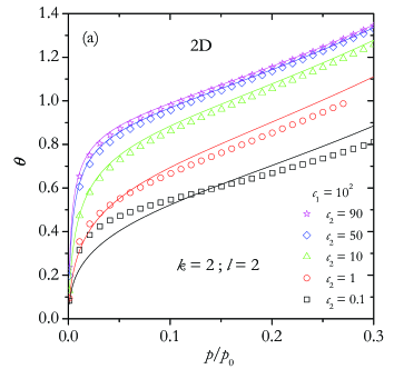
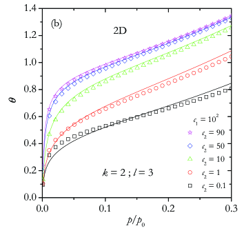
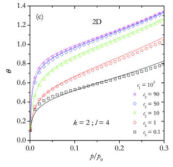
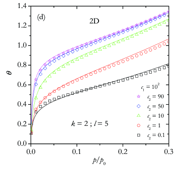
Figure 5: Comparison between approximate analytic and MC isotherms for dimers and different 2D heterogeneous surface: (a) $l=2$, (b) $l=3$, (c) $l=4$ and (d) $l=5$. In all cases, we have used lattices of size $L=240$ and $t=10^{5}$ MCSs.

Figure 4a shows the function $\Delta$ calculated from eq (16) for $c_{1}=10^{2}$, $c_{2}=1$ and different values of $k$ and $l$. As in the case of dimers, the difference between the analytic and the MC isotherms increases when $l$ is approximately a multiple of $k$. However, for large patches, i.e. $l>3k$, this difference becomes smaller. The inset shows, for a particular case ($k=10$ and $l=10$), how $\Delta$ diminishes as $c_{2}$ is increased. On the other hand, in Figure 4b we can see the function $\Delta$ calculated from eq (23). For $k>2$, the first peak is higher than the one shown in Figure 4a and is located in a value of $l/k$ between $0.5$ and $0.7$. Nevertheless, the oscillations attenuate quickly as the parameter $l/k$ is increased. As before, but now for $k=10$ and $l=5$, the inset shows how $\Delta$ diminishes as $c_{2}$ increases.

Finally, the analysis of Figure 4 indicates that, instead of eq (16) which has many terms, eq (23) can be used as a more simple expression to approach the 1D multilayer adsorption isotherm.

4.2 Adsorption on 2D Heterogeneous Surfaces

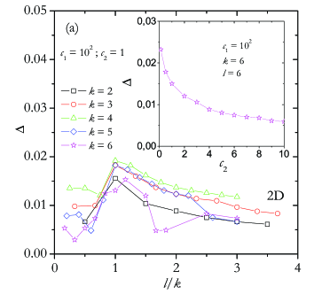
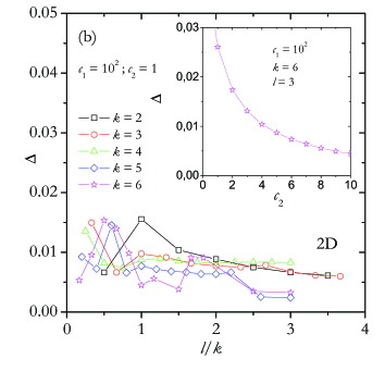
Figure 6: Function $\Delta$ vs $l/k$ for the adsorption in a 2D heterogeneous surface with $c_{1}=10^{2}$, $c_{2}=1$ and different values of $k$ as indicated. (a) Function $\Delta$ calculated from eq (16). The inset shows the dependence of $\Delta$ with $c_{2}$ for $k=6$ and $l=6$. b) Function $\Delta$ calculated with eq (23). The inset shows the dependence of $\Delta$ with $c_{2}$ for $k=6$ and $l=3$.

As in the homogeneous case, we represent the 2D surface by a square lattice with fully periodic boundary conditions. Strong and weak sites are spatially distributed in square patches of size $l$ forming a chessboard. Now, the total number of configurations of a single $k$-mer is $2M$. However, as before, only $2l$ terms are necessary to describe the multilayer isotherm. The explanation is quite simple: the available energies of a $k$-mer that it is forced to move in any direction of the lattice (row or column) are the same that in 1D. Then, eq (16) continues being valid in 2D, where the local isotherm is given by eqs (12) and (8), with $\gamma=4$.

We begin analyzing the multilayer isotherm for $k=2$ (for $k=1$, eq (19) continues being valid in 2D). Unfortunately, it is not possible to write a simple analytic expression [as eq (20)] in 2D. Nevertheless, the multilayer adsorption isotherm for dimers has the same structure that eq (20). Namely, it is composed by three terms with $c_{1}$, $c_{2}$ (both multiplied by $(l-1)/2l$) and $c=\sqrt{c_{1}c_{2}}$ (multiplied by $1/l$). Note that in 2D this function is approximate for any value of the parameter $l$.

Figures 5a, b, c and d show the multilayer isotherm for $c_{1}=10^{2}$ and different values of $l$ and $c_{2}$. The behavior of these curves is very similar to the one observed in 1D, but the difference between analytic and MC adsorption isotherms (for even and odd values of $l$) is no longer so important. On the other hand, Figures 6a and b show the dependence of the function $\Delta$ on $l/k$, where $\Delta$ was calculated by using eq (16) and eq (23), respectively. As in the case of 2D homogeneous surfaces, the analytic isotherm does not fit very well the MC data for $k>6$. For this reason, Figures 6a and b show the function $\Delta$ up to $k=6$ only.

In addition, we have shown that just by using an expression of three terms, eq (23), we can approach very well the multilayer isotherm in 1D and 2D for the adsorption on heterogeneous surfaces. In the next section, we will use this approximation and MC simulations to study how the topography affects the determination of monolayer volume predicted by the BET equation.

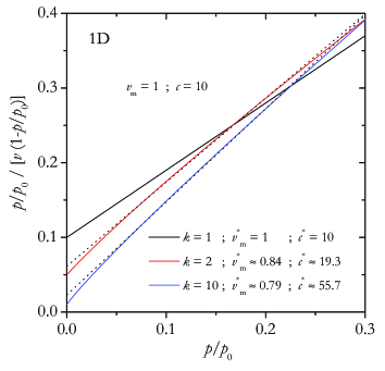
Figure 7: BET plots for 1D analytic isotherms of $k$-mers with $v_{\mathrm{m}}=1$, $c=10$ and different values of $k$ as indicated. Dotted lines correspond to linear fits of the data in the range $0.05$ to $0.25$.

5 Monolayer Volume

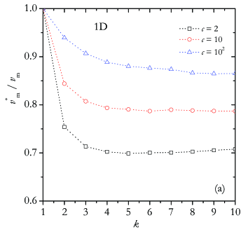
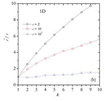
Figure 8: Results of the BET plots for the adsorption in 1D homogeneous surfaces. Dependence on $k$ of the fractions (a) $v_{\mathrm{m}}^{*}/v_{\mathrm{m}}$ and (b) $c^{*}/c$, for three different values of $c$ as indicated.

In this section, we carry out numerical experiments to determine, in different adsorption situations, how much the value of the monolayer volume predicted by the BET equation differs from its real value, $v_{\mathrm{m}}$. With this purpose, analytic and MC isotherms were analyzed as experimental data. In this way, we have determined how adsorbate size, energetic heterogeneity and surface topography affect the standard determination of the monolayer volume.

In a typical experiment of adsorption, the adsorbed volume of the gas, $v$, is measured at different pressures and at a given fixed temperature. In terms of this quantity, the total coverage is $\theta=v/v_{\mathrm{m}}$. Analyzing an isotherm with the BET equation, it is possible to estimate the monolayer volume. We rewrite the eq (4) as

$$\frac{p/p_{0}}{v\left(1-p/p_{0}\right)}=\frac{1}{cv_{\mathrm{m}}}+\frac{\left(c-1\right)}{cv_{\mathrm{m}}}p/p_{0}.$$ (25)

This equation is a linear function of $p/p_{0}$. If we denote with $a$ and $b$, the $y$-intercept and the slope of this straight line, respectively, we obtain

$$v_{\mathrm{m}}^{*}=\frac{1}{a+b}$$ (26)

and

$$c^{*}=\frac{b}{a}+1.$$ (27)

The asterisk has been added in order to indicate that the quantities given by eqs (26) and (27) correspond to the prediction of the BET theory. Then, by means of a plot (the so-called BET plot) of the experimental data of $\frac{p/p_{0}}{v\left(1-p/p_{0}\right)}$ vs $p/p_{0}$, we can obtain an estimate of the monolayer volume and the parameter $c$. Nevertheless, in the experiments it is commonly found that there are deviations from linearity in the BET plot. In many cases, the linear range extends from a relative pressure of $0.05$ to $0.35$, although there are cases where the range is shorter. [1]

Although the BET plot is a very simple and popular protocol, the value of the monolayer volume obtained in this way can differ from its real value. As mentioned in the introduction, in an interesting numerical experiment, [8] Walker and Zettlemoyer analyzed a BET plot of an analytic isotherm composed by two BET-like contributions (a isotherm similar to eq (19) for a LPT), each one with different values of $v_{\mathrm{m}}$ and $c$. The authors concluded that the application of the conventional BET equation to this heterogeneous isotherm may lead to an underestimate of the true monolayer volume, with a $c$ lying between the values for the two type of sites. Later, Cortés and Araya [9] have obtained a similar result by averaging the BET equation with a Gaussian distribution of adsorption energy. More recently Nikitas, [10] has arrived to similar conclusions by considering both, surface heterogeneity and polyatomic character of the adsorbate.

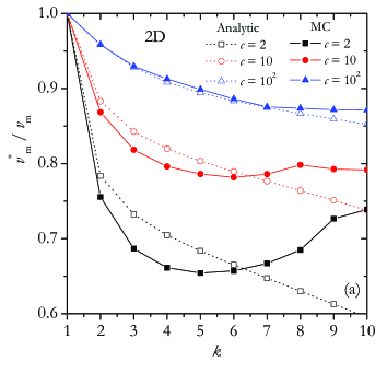
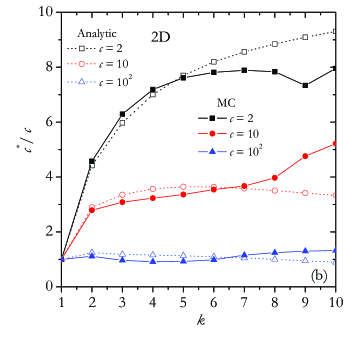
Figure 9: Results of the BET plots for the adsorption in 2D homogeneous surfaces. Dependence on $k$ of the fractions (a) $v_{\mathrm{m}}^{*}/v_{\mathrm{m}}$ and (b) $c^{*}/c$, for three different values of $c$ as indicated.

In the following, we will show that even for adsorption over homogeneous surfaces, the polyatomic character of the adsorbate affects significantly the predictions of a BET plot. Next, in Section 5.2, by considering bivariate surfaces, we will study the combined effect of energetic heterogeneity and multisite occupancy.

5.1 Homogeneous Surfaces

We begin analyzing the BET plots of the multilayer adsorption of $k$-mers over homogeneous surfaces, given by eqs (8) and (12) and MC data. Although in each particular case it is possible to find an optimum range of relative pressures, for practical purposes, we have chosen to set this range from $0.05$ to $0.25$. Nevertheless, by choosing other ranges (for example, between $0.05$ and $0.35$) we obtain similar results.

In Figure 7 we show the BET plot for 1D analytic isotherms with $c=10$ and $k=1$, 2 and 10. Note the deviations from linearity in the isotherms for $k=2$ and 10, which are concave to the pressure axis. The same behavior is observed in experimental isotherms and it is attributed to the existence of surface heterogeneities. [8] However, as we see in the example shown in Figure 7, these deviations also appear for the multilayer adsorption with multisite occupancy on a homogeneous surface.

On the other hand, as indicated in Figure 7, the obtained value of $v_{\mathrm{m}}^{*}$ for $k>1$ is smaller than the real one (we set $v_{\mathrm{m}}=1$), while the opposite effect is observed in the estimate of the parameter $c$. Figures 8a and b show the dependence of these quantities on $k$ for different values of $c$. In all cases, we obtain $v_{\mathrm{m}}^{*}\leq v_{\mathrm{m}}$ and $c^{*}\geq c$, but the differences between the BET predictions and the real values are smaller with increasing $c$.

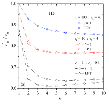
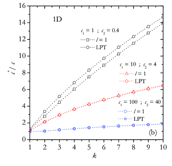
Figure 10: Results of the BET plots for the adsorption in 1D heterogeneous surfaces with $l=1$ and LPT. Dependence on $k$ of the fractions (a) $v_{\mathrm{m}}^{*}/v_{\mathrm{m}}$ and (b) $c^{*}/c$, for three different values of $c_{1}$ and $c_{2}$ (being $c_{1}/c_{2}=2.5$) as indicated.

Similar results have been obtained in 2D: the BET plots of both analytic and MC isotherms show the same curvature as found in 1D. Figures 9a and b show the results of these 2D BET plots. As we can see, the differences between analytic and MC isotherms are significant for small values of $c$. However, always $v_{\mathrm{m}}^{*}\leq v_{\mathrm{m}}$ and $c^{*}\geq c$ for $k>1$. As in the 1D case, the monolayer volume predicted by BET is approximately 10-30 per cent smaller than the real value.

5.2 Heterogeneous Surfaces

In previous work, [8, 9] it has been determined that, as heterogeneous adsorption isotherms of monomers are analyzed, the monolayer volume obtained from a BET plot is smaller than the real value. Since in this case $k=1$, the surface topography does not affect the obtained results. In this section, we study the dependence of the monolayer volume on both, adsorbate size and surface topography. In particular, we analyze analytic and MC adsorption isotherms of $k$-mers over bivariate surfaces with $l=1$ and LPT.

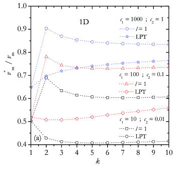
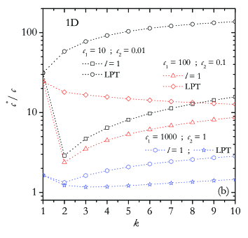
Figure 11: Results of the BET plots for the adsorption in 1D heterogeneous surfaces with $l=1$ and LPT. Dependence on $k$ of the fractions (a) $v_{\mathrm{m}}^{*}/v_{\mathrm{m}}$ and (b) $c^{*}/c$, for three different values of $c_{1}$ and $c_{2}$ (being $c_{1}/c_{2}=10^{3}$) as indicated.

Figures 10a and b show the results of the 1D BET plots for three different values of $c_{1}$ and $c_{2}$, being $c_{1}/c_{2}=2.5$. In this case, only analytic isotherms were studied because they are exact for LPT and the agreement with MC data is seen to be remarkably good for $l=1$ [except for odd values of $l$ ($l>1$), as was previously mentioned]. In all cases we have used $c=\sqrt{c_{1}c_{2}}$ as the reference parameter. As we can see, the curves show that there is not a significant difference between both topographies. Only when the quotient between $c_{1}$ and $c_{2}$ is increased, the space distribution of the adsorption energies over the solid surface begins to be important. This is shown in Figures 11a and b, where $c_{1}/c_{2}=10^{3}$. The results of the BET plots for $l=1$ and LPT are very different. For $c_{1}=10$ and $c_{2}=0.01$, the deviations due to molecule size $k$ are increased in LPT, i. e. the monolayer volume and the parameter $c$ obtained from a BET plot are, respectively, smaller and larger than the real values (or the reference value). However, most of the curves show a compensation effect which is larger for $l=1$, and for $c_{1}=10^{3}$ and $c_{2}=1$.

Finally, Figures 12a and b, and Figures 13a and b show the results of the 2D BET plots for $c_{1}/c_{2}=2.5$ and $c_{1}/c_{2}=10^{3}$, respectively. In all cases, we have analyzed both analytic and MC isotherms. As we can see, the behavior is similar to the 1D case. Nevertheless, even taking very different values of the parameters $c_{1}$ and $c_{2}$, it is not possible to obtain a complete compensation effect.

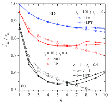
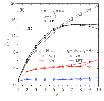
Figure 12: Results of the BET plots for the adsorption in 2D heterogeneous surfaces with $l=1$ and LPT. Open (full) symbols show results obtained from the analytic (MC) isotherms. Dependence on $k$ of the fractions (a) $v_{\mathrm{m}}^{*}/v_{\mathrm{m}}$ and (b) $c^{*}/c$, for three different values of $c_{1}$ and $c_{2}$ (being $c_{1}/c_{2}=2.5$) as indicated.

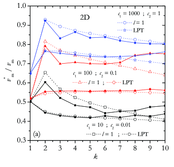
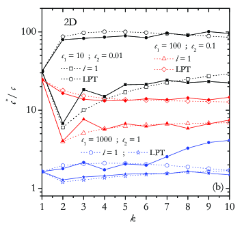
Figure 13: Results of the BET plots for the adsorption in 2D heterogeneous surfaces with $l=1$ and LPT. Open (full) symbols show results obtained from the analytic (MC) isotherms. Dependence on $k$ of the fractions (a) $v_{\mathrm{m}}^{*}/v_{\mathrm{m}}$ and (b) $c^{*}/c$, for three different values of $c_{1}$ and $c_{2}$ (being $c_{1}/c_{2}=10^{3}$) as indicated.

6 Conclusions

In the present paper, an analytic isotherm for the multilayer adsorption of polyatomic molecules on different surfaces has been proposed. The formalism reproduces the classical BET theory [6] and the recently reported dimer equations; [11] leads to the exact solution for a 1D homogeneous substrate; and, as is demonstrated from comparison with MC simulation, provides a good approximation for 1D heterogeneous surfaces. With respect to 2D substrates (homogeneous and heterogeneous surfaces), the approach is not exact. However, MC data shows that, for molecules of moderate size (not larger than $k=6$), the analytic isotherm behaves qualitatively similar to the simulation.

In addition, we carry out numerical experiments to determine, in different adsorption situations, how much the value of the monolayer volume predicted by the BET equation differs from its real value. For this purpose, analytic isotherms and MC data were analyzed as experimental data. For 1D and 2D homogeneous surfaces, the monolayer volume calculated by the BET plots is approximately 10-30 per cent smaller than the real value. On the other hand, in all cases, the parameter $c^{*}$ is always larger than $c$. As the multilayer adsorption occurs on a bivariate heterogeneous surface, a compensation effect is found, with very different values of $c$. Nevertheless, in any of the considered cases, this compensation is not enough to eliminate the decrease caused by the molecular size.

References

- [1] Gregg, S. J.; Sing, K. S. W. Adsorption, Surface Area and Porosity; Academic Press: New York, 1991.
- [2] Rudzinski, W.; Everett, D. H. Adsorption of Gases on Heterogeneous Surfaces; Academic Press: London, 1992.
- [3] Frenkel, J. Kinetic Theory of Liquids; Clarendon Press: Oxford, 1946; Dover reprint: New York, 1955.
- [4] Halsey, G. D. J. Chem. Phys. 1948, 16, 931.
- [5] Hill, T. L. Adv. Catal. 1952, 4, 211.
- [6] Brunauer, S.; Emmett, P. H.; Teller, E. J. Am. Chem. Soc. 1938, 60, 309.
- [7] Hill, T. L. An Introduction to Statistical Thermodynamics; Addison Wesley Publishing Company: Reading, MA, 1962.
- [8] Walker, W. C.; Zettlemoyer, A. C. J. Phys. Coll. Chem. 1948, 52, 47.
- [9] Cortés, J.; Araya, P. J. Coll. Interface Sci. 1987, 115, 271.
- [10] Nikitas, P. J. Phys. Chem. 1996, 100, 15247.
- [11] Riccardo, J. L.; Ramirez-Pastor, A. J.; Romá, F. Langmuir 2002, 18, 2130.
- [12] Romá, F.; Ramirez-Pastor, A. J.; Riccardo, J. L. Surf. Sci. 2005, 583, 213.
- [13] Somorjai, G. A.; Van Hove, M. A. Adsorbed Monolayers on Solid Surfaces; Springer-Verlag: Berlin, 1979.
- [14] Ramirez-Pastor, A. J.; Eggarter, T. P.; Pereyra, V. D.; Riccardo, J. L. Phys. Rev. B 1999, 59, 11027.
- [15] Romá, F.; Riccardo, J. L.; Ramirez-Pastor, A. J. Langmuir 2006, 22, 3192.
- [16] Riccardo, J. L.; Romá, F.; Ramirez-Pastor, A. J. Int. J. of Mod. Phys. B 2006, 20, 4709.
- [17] Riccardo, J. L.; Chade, M. A.; Pereyra, V. D.; Zgrablich, G. Langmuir 1992, 8, 1518.
- [18] Bulnes, F.; Ramirez-Pastor, A. J.; Zgrablich, G. J. of Chem. Phys. 2001, 115, 1513.