EL MÉTODO DE PATRONES ESTANDARIZABLES PARA
SUPERNOVAS TIPO II-PLATEAU

Abstract

Durante el desarrollo de esta tesis estudiamos el Método de Patrones Lumínicos Estandarizables (SCM) para supernovas Tipo II “plateau” haciendo uso de fotometría $BVRI$ y espectroscopía óptica. Se implementó un procedimiento analítico para ajustar funciones a las curvas de luz, de color y de velocidad de expansión. Encontramos que el color $V$ – $I$ de estas supernovas, medido hacia el final de la época “plateau”, puede ser utilizado para estimar el enrojecimiento provocado por el material interestelar de la galaxia anfitriona con una precisión de $\sigma(A_{V})=0.2$ mag. Tras realizar las correcciones necesarias a la fotometría se recupera la relación luminosidad versus velocidad de expansión, reportada previamente en la literatura científica. Ocupando esta relación y asumiendo una ley de extinción estándar ($R_{V}=3.1$) obtenemos diagramas de Hubble con dispersiones de $\sim$ 0.4 mag en las bandas $BVI$. Por otra parte, si permitimos variaciones en $R_{V}$ en favor de incertezas menores obtenemos una dispersión final de 0.25–0.30 mag, lo que implica que estos objetos pueden entregar distancias tan precisas como 12–14%. El valor resultante para $R_{V}$ es de $1.4\pm 0.1$, que sugiere una ley de extinción no-estándar en nuestra línea de visión hacia este tipo de supernovas. Utilizando dos objetos con distancia Cefeida para calibrar la relación luminosidad-velocidad obtenemos una constante de Hubble de $70\pm 8$ km s^-1 Mpc^-1, en buen acuerdo con el valor que obtuvo el HST Key Project.

Quiero agradecer en primer lugar a mi amada mujer, Natalia Armijo, quien logró mantenerme enfocado y motivado. Su constante apoyo fue vital para mi constancia. Junto con mi familia jugaron el importante rol de estar incondicionalmente presentes, respaldándome. Esas visitas de fin de semana a la casa de mi familia en Valparaíso fueron una contribución infalible en favor del relajo y en contra del estrés. Mi hermano Sebastián, mi abuela Mariana y mi madre Ana María me recibieron siempre con los brazos abiertos. En especial mi madre, quién fue crucial al momento de empezar mis estudios fuera de casa. Sin su constante apoyo no hubiese podido sobrellevar la complicada vida del estudiante de provincia en Santiago. Muchas gracias también a todos mis amigos, de quienes recibí mucha ayuda a la hora de despejar la mente. En cuanto a lo académico, muchos de mis conocimientos e ideas impregnadas en esta tesis fueron responsabilidad de mi profesor guía, Mario Hamuy, quién consiguió transmitirme todo su entusiasmo, ideas innovadoras y experiencia. Le agradezco a Mario el haberme llevado por el mejor camino hacia la obtención de mi grado. Además quiero agradecer el apoyo del Centro Milenio para Estudios de Supernovas a través del subsidio P06–045–F financiado por el “Programa Bicentenario de Ciencia y Tecnología de CONICYT” y por el “Programa Iniciativa Científica Milenio de MIDEPLAN”, y el apoyo recibido por parte del Centro de Astrofísica FONDAP 15010003 y de Fondecyt a través del subsidio 1060808.

Para mi madre,
sin ella nada de esto hubiese sido posible.

Chapter 0 Introduction

Supernovae (hereafter SNe) correspond to the explosive, high-energy final stages of some stars. The mechanical energy released in these powerful events can reach as much as 10⁵¹ erg (or 1 foe), and their peak luminosities can be comparable to the total light of their host-galaxies. SNe can be classified in two types, either “Core Collapse” or “Thermonuclear”, depending on their explosion mechanisms.

Core-collapse SNe (CCSNe) are closely associated to star forming regions in late-type galaxies (Anderson & James 2008). Therefore they have been attributed to massive stars born with $>$ 8 M_⊙ that undergo the collapse of their iron cores after a few million years of evolution and the subsequent ejection of their envelopes (Burrows 2000). These SNe leave a compact object as a remnant, either a neutron star or a black hole (Baade & Zwicky 1934; Arnett 1996). The core-collapse model received considerable support with the first detection of neutrinos from the Type II SN 1987A (Svoboda et al. 1987), although no compact remnant has been found so far in the explosion site. Among CCSNe we can observationally distinguish those with prominent hydrogen lines in their spectra (dubbed Type II), those with no H but strong He lines (Type Ib), and those lacking H or He lines (Type Ic) (Minkowski 1941; Filippenko 1997). Although all of these objects are thought to share the same explosion mechanism, their different observational properties are explained in terms of how much of their H-rich and He-rich envelopes were retained prior to explosion. When the star explodes with a significant fraction of its initial H-rich envelope, in theory it should display a H-rich spectrum and a light curve characterized by a phase of $\sim$ 100 days of nearly constant luminosity followed by a sudden drop of 2–3 mag (Nadyozhin 2003; Utrobin 2007; Bersten et al. 2008). Nearly 50% of all CCSNe belong to this class of Type II “Plateau” SNe (SNe II-P).

Thermonuclear SNe are characterized by the lack of hydrogen and helium in their spectra. Their early-time spectra show strong lines due to intermediate mass elements (e.g. Si 2, Ca 2, Mg 2; Filippenko 1997). They are found both in elliptical, spiral, or irregular galaxies. These objects are thought to originate in low-mass stars that end their lifes as white dwarfs and explode after a period of mass accretion from a companion star, leaving no compact remnants behind them (Hillebrandt & Niemeyer 2000). Observationally they are referred as Type Ia SNe.

Given their large intrinsic luminosities, SNe have long been considered potential probes for extra-galactic distance determinations and the measurement of the cosmological parameters that drive the Universe dynamics. Among all types of SNe, the Type Ia family is the one displaying the highest degree of homogeneity (Li et al. 2001), both photometrically and spectroscopically. However, these objects are not perfect standard candles. Empirical calibrations have allowed us to standardize their luminosities to levels of $\sim$ 0.15–0.22 mag and determine distances to their host-galaxies with an unrivaled precision of $\sim$ 7%–10% (Phillips 1993; Hamuy et al. 1996; Phillips et al. 1999). This powerful technique led a decade ago to the construction of Hubble diagrams between $z=0$–0.5 and measure very precisely the history of the expansion of the Universe over 5 Gyr of look-back time. Contrary to our intuition these observations revealed that the Universe dynamics is described by an accelerated expansion (Riess et al. 1998; Perlmutter et al. 1999; Astier et al. 2006; Wood-Vasey et al. 2007). The discovery of the accelerating Universe is profoundly connected with theoretical cosmology as it implies the possible existence of a cosmological constant, a concept initially introduced by Albert Einstein at the beginning of the 20th century, whose origin still is a mystery.

Although the acceleration of the Universe has been indirectly confirmed by other independent experiments such as the Wilkinson Microwave Anisotropy Probe (WMAP; Spergel et al. 2007; Bennett et al. 2003) and the Baryon Accoustic Oscillations (BAO; Blake & Glazebrook 2003; Seo & Eisenstein 2003), it is important to obtain independent confirmation of the Type Ia results. Although not as bright and uniform as the Type Ia’s, Hamuy & Pinto (2002) showed that the luminosities of SNe II-P can be standardized to levels of 0.4 and 0.3 mag in the $V$- and $I$-bands respectively, thus converting these objects into potentially useful tools to measure cosmological parameters.

Even though SNe II-P are 1–2 mag fainter and much less homogeneous than SNe Ia, these objects provide two interesting routes to distance determinations. First, the Expanding Photosphere Method (EPM, Kirshner & Kwan 1974), a theoretical technique based on atmosphere models that is independent of the extra-galactic distance scale (Eastman et al. 1996; Dessart & Hillier 2005). This method can achieve dispersions of 0.3 mag in the Hubble diagram, which translates into a 14% precision in distance (Schmidt et al. 1994; Hamuy 2001; Jones et al. 2008). Second, the Standardized Candle Method (SCM for short), an empirical technique initially proposed by Hamuy & Pinto (2002) that is based on an observational correlation between the absolute magnitude of the SN and the expansion velocity of the photosphere, the Luminosity-Expansion Velocity ($LEV$) relation. This correlation shows that SNe II-P with greater luminosities have higher expansion velocities, which permits one to remove the large ($\sim$ 4 mag) luminosity differences displayed by these objects to levels of only 0.3 mag. So far, the SCM has been applied to 24 low-$z$ ($z<0.05$) SNe (Hamuy 2003) and more recently by Nugent et al. (2006) to 5 high-$z$ ($z<0.29$) SNe. The latter work was the first attempt to derive cosmological parameters from SNe II-P and demonstrated the enormous potential of this class of objects as cosmological probes.

The upcoming years will witness the deployment of several survey telescopes, such as the Panoramic Survey Telescope and Rapid Response System (Pan-STARRS; Hodapp et al. 2004), the Large Synoptic Survey Telescope (LSST; Tyson et al. 2003), the Visible and Infrared Survey Telescope (VISTA; Emerson et al. 2004), the VLT Survey Telescope (VST; Capaccioli et al. 2003), the Dark Energy Survey (DES; Castander 2007), and the Skymapper (Granlund et al. 2006), all of which offer the promise to discover SNe by the thousands. Whether we use it or not, we will be inevitably confronted by enormous amounts of data on SNe II-P which will contain valuable cosmological information. In spite of the great promise shown by the SCM, it still suffers from a variety of problems which need to be addressed: 1) the lack of a well-defined maximum in the light curves has prevented us from defining the phase of each event; 2) each SN shows a different color evolution, which has compromised the use of the photometric data for the determination of host-galaxy extinction; 3) the assumption for dereddening employed by Hamuy & Pinto (2002), namely that all SNe reach the same asymptotic color toward the end of the plateau phase, has often led to negative extinctions so it still needs to be further tested; 4) the small sample size used so far, especially the scarcity of SNe in the Hubble flow, has prevented a proper determination of the intrinsic precision of the method.

The purpose of this research is to take advantage of the larger and more distant sample of SNe II-P available to us today to address the issues mentioned above, refine the SCM, and assess the feasibility of using SNe II-P to measure distances in the Universe, in preparation for the massive samples of high-$z$ SNe which will be produced in the years to come. With this purpose in mind we have developed a robust mathematical procedure to model the light curves, color curves, and velocity curves, in order to obtain a more accurate determination of the relevant parameters required by the SCM (magnitudes, colors and ejecta velocities). This work makes use of 37 SNe to construct a Hubble diagram (HD), evaluate the accuracy of the SCM, and obtain an independent determination of the Hubble constant. Since our sample has several objects in common with the recent EPM analysis of Jones et al. (2008), we perform a comparison between SCM and EPM.

We organize this thesis as follows. In § 1 we describe all of the observational material used in this work such as the telescopes, intruments and surveys involved. The analysis, methodology and procedures, such as the $A_{G},\ K$ and $A_{host}$ corrections, are explained in detail in § 2. The dereddening analysis, the Hubble diagram, the value of the Hubble constant, and the distance comparison between SCM and EPM are addressed in § 3. The final remarks in § 4 provide a discussion about possible variations of the reddening law for SNe II-Palong with comparisons between the value of $H_{0}$ computed by us and those derived from other methods. The first part of this section explores the possibility of a non-standard extinction law in the SN host-galaxies. We present our conclusions in § 5.

Chapter 1 Observational Material

This work makes use of data obtained in the course of four systematic SN follow-up programs carried out between 1986–2003: 1) the Cerro Tololo SN program (1986–1996); 2) the Calán/Tololo SN program (CT, 1990–1993); 3) the Optical and Infrared Supernova Survey (SOIRS, 1999–2000); 4) the Carnegie Type II Supernova Program (CATS, 2002–2003). As a result of these efforts photometry and spectroscopy (some IR but mostly optical) was obtained for nearly 100 SNe of all types, 51 of which belong to the Type II class. All of the optical data have been already reduced and they are being prepared for publication (Hamuy et al. 2008). Next we describe in general terms the data acquisition and reduction procedures. For more details the reader can refer to Hamuy et al. (2008).

1 Photometric Data

The photometry was acquired with telescopes from Cerro Tololo Inter-American Observatory (CTIO), Las Campanas Observatory (LCO), the European Southern Observatory (ESO) in La Silla, and Steward Observatory (SO). A host of different telescopes and intruments were used to generate this dataset as shown in Table 1. In all cases we employed CCD detectors and standard Johnson-Kron-Cousins-Hamuy $UBVRIZ$ filters (Johnson et al. 1966; Cousins 1971; Hamuy et al. 2001).

Table 1: Telescopes and instruments

Telescope	Instrument	Phot/Spec
CTIO 0.9m	CCD	P
YALO 1.0m	ANDICAM	P
YALO 1.0m	2DF	S
CTIO 1.5m	CCD	P
CTIO 1.5m	CSPEC	S
Blanco 4.0m	CSPEC	S
Blanco 4.0m	2DF	S
Blanco 4.0m	CCD	P
Swope 1.0m	CCD	P
du Pont 2.5m	WFCCD	P/S
du Pont 2.5m	MODSPEC	S
du Pont 2.5m	2DF	S
du Pont 2.5m	CCD	P
Baade 6.5m	LDSS2	P/S
Baade 6.5m	B&C	S
Clay 6.5m	LDSS2	P/S
ESO 1.52m	IDS	S
Danish 1.54m	DFOSC	P/S
ESO 2.2m	EFOSC2	S
NTT 3.58m	EMMI	S
ESO 3.6m	EFOSC	S
Kuiper 61”	CCD	P
Bok 90”	B&C	S

The images were processed with IRAF through bias subtraction and flatfielding. All of them were further processed through the step of galaxy subtraction using template images of the host-galaxies. Photometric sequences were established around each SN based on observations of Landolt and Hamuy standards (Landolt 1992; Hamuy et al. 1992, 1994). The photometry of all SNe was performed differentially with respect to the local sequence on the galaxy-subtracted images. The transformation of instrumental magnitudes to the standard system was done by taking into account a linear color-term and a zero-point. Although this procedure partially removes the instrument-to-instrument differences in the SN magnitudes, it should be kept in mind that significant systematic discrepancies can still remain owing to the non-stellar nature of the SN spectrum (e.g.  Hamuy et al. 1990).

2 Spectroscopic Data

The spectroscopic data were also obtained with a great variety of instruments and telescopes as shown in Table 1. The observations consisted of the SN observation immediately followed by an arc lamp taken at the same position in the sky, and 2–3 flux standards per night from the list of Hamuy et al. (1992, 1994).

We always used CCD detectors, in combination with different gratings/grisms and blocking filters. The reductions were performed with IRAF and consisted in bias subtraction, flatfielding, 1D spectrum extraction and sky subtraction, wavelength and flux calibration. No attempts were done to remove the telluric lines.

3 Subsample used for this work

Of the 51 SNe II observed in the course of these four surveys, a subset of 33 objects comply with the requirements of 1) having light curves with good temporal coverage; 2) having sufficient spectroscopic temporal coverage; 3) being a member of the plateau class. To this sample we added four SNe from the literature: SN 1999gi, SN 2004dj, SN 2004et, and SN 2005cs. Complementary photometry for SN 2003gd obtained by Van Dyk et al. (2003) and Hendry et al. (2005) was also incorporated in our analysis. Table 2 lists our final sample of 37 SNe II-P. For each SN this table includes the name of the host-galaxy, equatorial coordinates, the heliocentric redshift and its source, the reddening due to our own Galaxy (Schlegel et al. 1998) and the survey or reference for the data.

Table 2: Supernova sample

SN name	Host Galaxy	RA(J2000)	DEC(J2000)	$z_{host}$	(s)	$E(\mbox{$B\!-\!V$})_{GAL}$	References
1991al	LEDA 140858	19 42 24.00	–55 06 23.0	0.01525	HP02	0.051	1
1992af	ESO 340-G038	20 30 40.20	–42 18 35.0	0.01847	NED	0.052	1
1992am	MCG–01–04–039	01 25 02.70	–04 39 01.0	0.04773	NED	0.049	1
1992ba	NGC 2082	05 41 47.10	–64 18 01.0	0.00395	NED	0.058	1
1993A	$anonymous$	07 39 17.30	–62 03 14.0	0.02800	NED	0.173	1
1999br	NGC 4900	13 00 41.80	+02 29 46.0	0.00320	NED	0.024	2
1999ca	NGC 3120	10 05 22.90	–34 12 41.0	0.00931	NED	0.109	2
1999cr	ESO 576–G034	13 20 18.30	–20 08 50.0	0.02020	NED	0.098	2
1999em	NGC 1637	04 41 27.04	–02 51 45.2	0.00267	NED	0.040	2
1999gi	NGC 3184	10 18 17.00	+41 25 28.0	0.00198	NED	0.017	3
0210	MCG +00–03–054	01 01 16.80	–01 05 52.0	0.05140	NED	0.036	4
2002fa	NEAT J205221.51	20 52 21.80	+02 08 42.0	0.06000	NED	0.099	4
2002gw	NGC 922	02 25 02.97	–24 47 50.6	0.01028	NED	0.020	4
2002hj	NPM1G +04.0097	02 58 09.30	+04 41 04.0	0.02360	NED	0.115	4
2002hx	PGC 23727	08 27 39.43	–14 47 15.7	0.03099	NED	0.054	4
2003B	NGC 1097	02 46 13.78	–30 13 45.1	0.00424	NED	0.027	4
2003E	MCG–4–12–004	04 39 10.88	–24 10 36.5	0.01490	J08	0.048	4
2003T	UGC 4864	09 14 11.06	+16 44 48.0	0.02791	NED	0.031	4
2003bl	NGC 5374	13 57 30.65	+06 05 36.4	0.01459	J08	0.027	4
2003bn	2MASX J10023529	10 02 35.51	–21 10 54.5	0.01277	NED	0.065	4
2003ci	UGC 6212	11 10 23.83	+04 49 35.9	0.03037	NED	0.060	4
2003cn	IC 849	13 07 37.05	–00 56 49.9	0.01811	J08	0.021	4
2003cx	NEAT J135706.53	13 57 06.46	–17 02 22.6	0.03700	NED	0.094	4
2003ef	NGC 4708	12 49 42.25	–11 05 29.5	0.01480	J08	0.046	4
2003fb	UGC 11522	20 11 50.33	+05 45 37.6	0.01754	J08	0.183	4
2003gd	M74	01 36 42.65	+15 44 20.9	0.00219	NED	0.069	4, 5, 6
2003hd	MCG–04–05–010	01 49 46.31	–21 54 37.8	0.03950	NED	0.013	4
2003hg	NGC 7771	23 51 24.13	+20 06 38.3	0.01427	NED	0.074	4
2003hk	NGC 1085	02 46 25.76	+03 36 32.2	0.02265	NED	0.037	4
2003hl	NGC 772	01 59 21.28	+19 00 14.5	0.00825	NED	0.073	4
2003hn	NGC 1448	03 44 36.10	–44 37 49.0	0.00390	NED	0.014	4
2003ho	ESO 235–G58	21 06 30.56	–48 07 29.9	0.01438	NED	0.039	4
2003ip	UGC 327	00 33 15.40	+07 54 18.0	0.01801	NED	0.066	4
2003iq	NGC 772	01 59 19.96	+18 59 42.1	0.00825	NED	0.073	4
2004dj	NGC 2403	07 37 17.00	+65 35 58.1	0.00044	NED	0.040	7
2004et	NGC 6946	20 35 25.30	+60 07 18.0	0.00016	NED	0.342	8
2005cs	NGC 5194	13 29 53.40	+47 10 28.0	0.00154	NED	0.035	9, 10

Chapter 2 Methodology and Procedures

1 AKA corrections

The photon flux measured by an observer is related to the intrinsic luminosity of the source, its distance, dust extinction along the line of sight, and the shift of the spectral energy distribution (SED) to longer wavelengths caused by the expansion of the Universe. More specifically, if $L_{\lambda^{\prime}}$ is the SN rest-frame emergent luminosity in units of $erg~{}s^{-1}~{}$Å^-1, the photon flux per unit wavelength seen by the observer (in units of $photons~{}cm^{-2}~{}s^{-1}~{}$Å^-1), is

$$n(\lambda)=\frac{L_{\lambda^{\prime}}~{}(\lambda^{\prime}/hc)~{}A_{host}(\lambda^{\prime})~{}A_{G}(\lambda)}{4\pi{d_{L}}^{2}}$$ (1)

where $\lambda^{\prime}$ is the SN rest-frame wavelength, $\lambda$=$\lambda^{\prime}(1+z)$ is the observer’s wavelength, and $d_{L}$ is the luminosity distance to the source.

The flux is modified along its journey to the observer in the following order: host-galaxy reddening ($A_{host}$), redshift ($K$-term), and Galactic reddening ($A_{G}$) (or AKA, for short). In order to be able to extract the distance from the observed fluxes, it proves necessary to remove Nature’s imprint on the observed magnitudes in reverse order. To undo Nature’s work, we first need to correct the observed magnitudes for Galactic extinction ($A_{G}$), which is equivalent to moving the observer outside the Milky Way. Then we must move the observer just outside the host-galaxy, for which we must correct the spectrum for the redshift caused by the expansion of the Universe ($K$ correction). Finally, we must correct the magnitudes for host-galaxy extinction ($A_{host}$), which brings the observer to the SN rest-frame. For the latter step we used as a first approximation the reddenings determined by Dessart (2008). In a second iteration we applied our own reddenings (see § 3).

In this work the AKA corrections are computed numerically using a library of 196 SNe II-P optical spectra. Most of the spectra comes from our own database of 44 Type II SNe, 10 of which are not included in Table 2 (SN 1987A, SN 1988A, SN 1989L, SN 1990E, SN 1990K, SN 1993S, SN 1999eg, SN 2000cb, SN 2002gd, and SN 2003ib). These 10 additional objects belong to the Type II class, although do not comply with the requirements of § 3 to be included in this analysis. The database comprises spectra covering the plateau and nebular phases. Each spectrum is brought to the SN rest-frame, i.e., to redshift zero and null Galactic reddening using the redshifts and Galactic reddenings listed in Table 2. Also the spectra are corrected using our own host-galaxy reddenings, as determined below (see § 3).

1 $A_{G}$ corrections

We define the synthetic apparent Galactic extinction correction as the difference between the magnitude of an unextinguished SED and the magnitude of the extinguished SED, i.e.,

$$A_{G}(\overline{\lambda})=-2.5~{}log_{10}~{}\frac{\int L_{\lambda^{\prime}}~{}\lambda^{\prime}~{}A_{host}(\lambda^{\prime})~{}A_{G}(\lambda)~{}S(\lambda)~{}d\lambda}{\int L_{\lambda^{\prime}}~{}\lambda^{\prime}~{}A_{host}(\lambda^{\prime})~{}S(\lambda)~{}d\lambda}$$ (2)

where $S(\lambda)$ is the filter transmission function (see Appendix 6). We apply this definition to all the spectra of our library using the $BVRI$ bandpasses. Since the effective wavelength $\overline{\lambda}$ changes as the SN spectrum evolves, we expect the apparent $A_{G}$ to be a function of the color of the SED. To examine this point, Figure 1 shows $A_{G}(V)$ against $B\!-\!V$ for the specific case of $A_{G}^{true}(V)$ = 1 mag, where we identify with different colors spectra from the plateau and nebular phases.

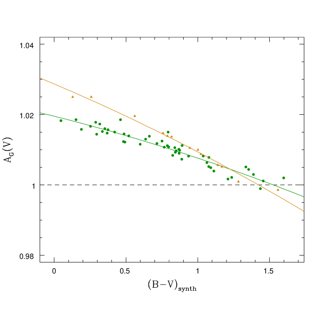
Figure 1: The dependence of the apparent $A_{G}(V)$ on the synthetic $B\!-\!V$ color obtained from the library of spectra must be taken into account. The dashed line defines the input $A_{G}^{true}(V)=1$ mag, indicating variations up to 0.025 mag. Plateau-phase spectra (filled circles) are shown and fitted in green, whereas the data from the nebular phase are shown with brown triangles. This diagram shows that the $A_{G}(V)$ versus $B\!-\!V$ calibration must be treated separately for the plateau and nebular phases.

Although the apparent $A_{G}$ does not show large variations, the dependence on color is evident and must be taken into account. For this purpose we chose to fit these relations with 3rd order polynomials. With this calibration we can proceed to interpolate the corresponding value of the apparent $A_{G}$ for the specific color of the SN and subtract this value from the observed magnitudes at every epoch we have photometry to obtain ($m_{obs}-A_{G}$). The RMS of our calibration —0.0008 mag— provides an estimate of the uncertainty in the correction, so we add this number in quadrature to the uncertainty in the observed magnitudes.

2 $K$ corrections

We use a similar procedure to compute the $K$ corrections. The synthetic $K$-term is defined as the difference between the magnitude of a redshifted SED and the magnitude of the zero-redshift SED, i.e.,

$$K(\overline{\lambda})=-2.5~{}log_{10}~{}\frac{\int L_{\lambda^{\prime}}~{}\lambda^{\prime}~{}A_{host}(\lambda^{\prime})~{}S(\lambda)~{}d\lambda}{\int L_{\lambda}~{}\lambda~{}A_{host}(\lambda)~{}S(\lambda)~{}d\lambda}$$ (3)

This definition is equivalent to that given by Schneider et al. (1983) except that they use fluxes per unit frequency. By definition the $K$-term is a color, therefore we expect it to correlate with the broad-band colors of the SED. To demonstrate this point, Figure 2 shows $K$ versus $B\!-\!V$ for the specific case of the $V$-band for $z$=0.05.

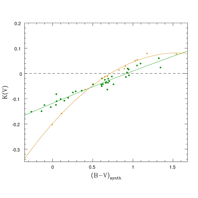
Figure 2: The dependence of $K(V)$ on the synthetic color $B\!-\!V$ obtained from the library of spectra. For a redshift of $z=0.05$ the $K$-terms reach absolute values up to 0.2 mag. Plateau-phase spectra (filled circles) are shown and fitted in green, whereas data from the nebular phase are shown with brown triangles. The diagram shows that the $K(V)$ versus $B\!-\!V$ calibration must be treated separately for the plateau and nebular phases.

This dependence is very useful as it permits us to interpolate $K$ values for the specific color of the SN and correct the photometry at the plateau or nebular phases separately. The result of this correction is the quantity ($m_{obs}-A_{G}-K$). The RMS of the points around the polynomial fits are of the order of $\sim$ 0.001–0.01 mag, and these are quadratically added to the error of ($m_{obs}-A_{G}$) in order to account for the uncertainties in the $K$ correction.

3 $A_{host}$ corrections

Finally, we must repeat the previous process for the $A_{host}$ correction. The following equation

$$A_{host}(\overline{\lambda})=-2.5~{}log_{10}~{}\frac{\int L_{\lambda}~{}\lambda~{}A_{host}(\lambda)~{}S(\lambda)~{}d\lambda}{\int L_{\lambda}~{}\lambda~{}S(\lambda)~{}d\lambda}$$ (4)

defines the apparent $A_{host}$ and gives the difference between the magnitude of the supernova right outside the host-galaxy ($m_{obs}-A_{G}-K$) and the magnitude free of host-galaxy dust ($m_{obs}-A_{G}-K-A_{host}$).

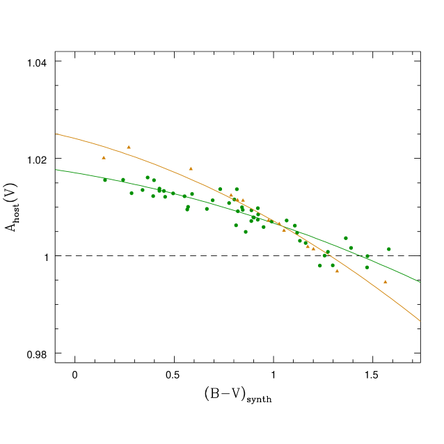
Figure 3: The dependence of the apparent $A_{host}(V)$ on the synthetic $B\!-\!V$ color obtained from the library of spectra. The dashed line defines the input $A_{host}^{true}(V)=1$, indicating variations up to 0.023 mag. Plateau-phase spectra (filled circles) are shown and fitted in green, whereas data from the nebular phase are shown in brown triangles. This diagram shows that the $A_{host}(V)$ versus $B\!-\!V$ calibration must be treated separately for the plateau and nebular phases.

Figure 3 shows this correction for all the plateau and nebular spectra of our library separately for the specific case $A_{host}^{true}(V)$ = 1 mag, which confirms the previous results, namely that the apparent $A_{host}$ is a function of the broad-band colors. We fit these relations with a 3${}^{\mbox{\scriptsize rd}}$ order polynomial and apply these calibrations to the SN magnitudes, making sure to include the RMS of the fits —varying between 0.003–0.01— in the error budget. At this point, we obtain the magnitude of the SN corrected for Galactic extinction, redshift and host-galaxy extinction for all epochs (colors) of the SN.

2 Fits to light, color and velocity curves

In the first incarnation of the SCM Hamuy & Pinto (2002) measured all the relevant quantities (magnitudes, colors and velocities) at fixed epochs with respect to the time of explosion. In most cases, however, it proves hard to constrain this time, thus hampering the task to compare data obtained for different SNe. It would be ideal to have a conspicuous feature in the light curves but, unlike other SN types, SNe II-P generally do not show an obvious maximum during the plateau phase.

One way around this is to use the end of the plateau as an estimate of the time origin for each event. Although simple in theory, in practice it is not easy to measure this time owing to the coarser sampling of the light curves at this phase. Thus, our first aim is to implement a robust light curve fitting procedure in order to obtain a reliable time origin to be used as a uniform reference epoch to measure magnitudes, colors, and expansion velocities. In the remainder of this section we proceed to implement fitting methods to measure reliable colors and expansion velocities.

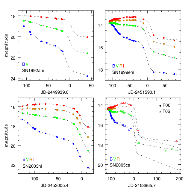
Figure 4: Four representative light curves of the SN sample. Data points are colored according to the filters. $BVRI$ magnitudes are respectively shown in blue, green, brown and red. The dotted line corresponds to the analytic fit (see Fig. 8). In the $B$ and $R$ light curve of SN 2005cs we can appreciate the quality of the procedure, since even without data points the code manages to achieve reasonable fits. The light curves of this SN were complemented with photometry from the literature (P06; Pastorello et al. 2006)(T06; Tsvetkov et al. 2006).

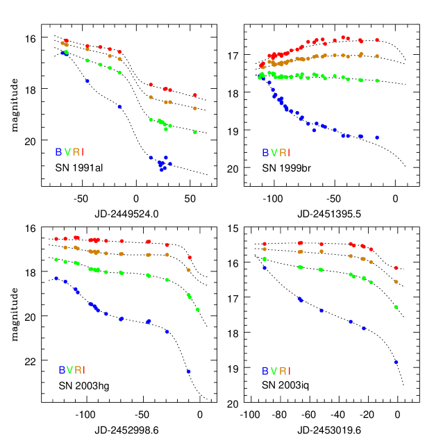
Figure 5: Four representative light curves of the SN sample. Data points are colored in the same way as in Fig. 4. The dotted line corresponds to the analytic fit (see Fig. 8).

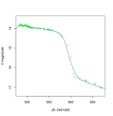
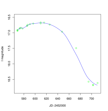
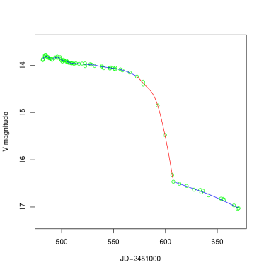
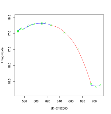
Figure 6: Loess fits to the $V$ light curve of SN 1999em (left panel) and to the $I$ light curve of SN 2002gw (right panel). Although the fits do a good job on small scales, the transition evidently is not well modelled.

Figure 7: Loess fits to the $V$ light curve of SN 1999em (left panel) and to the $I$ light curve of SN 2002gw (right panel). In this case the algorithm was applied separately to each phase (plateau, transition, and tail). Despite the satisfactory accuracy of the regression, we could not find an easy way to force the continuity at the two interfaces.

1 $BVRI$ light curve fits

Figures 4 and 5 show $BVRI$ light curves of eight well-observed SNe II-P. These SNe are representative of the whole sample. As can be seen, there are three distinguishable phases in the light curves:

—

The Plateau phase in which the SN shows an almost constant luminosity during the first $\sim$ 100 days of its evolution. This phase corresponds to the optically thick period in which a hydrogen recombination wave recedes in mass, gradually releasing the internal energy of the star (Nadyozhin 2003; Utrobin 2007; Bersten et al. 2008).

—

The Linear or Radioactive Tail, a linear decay in magnitude (exponential in flux) starting about 100 days after the explosion. This phase corresponds to the optically thin period powered by the ⁵⁶Co $\rightarrow$ ⁵⁶Fe radioactive decay (Weaver & Woosley 1980).

—

A Transition phase of $\sim$ 30 days between the plateau and linear phases.

Both the plateau and linear phases are trivial to model if taken separetely, but the abrupt transition makes the fitting task much more challenging, especially with coarsely sampled light curves. The first attempt consisted in using the Local Polynomial Regression Fitting, a technique developed by Cleveland et al. (1992) within the framework of the R environment for statistical computing. The name of the method is self-explanatory, since it performs a polynomial regression over small local intervals along the domain using a routine called loess. Figure 7 shows the resulting fits when all the data are fitted simultaneously by loess. The small scale features of the plateau are nicely reproduced, but loess is unable to model the transition satisfactorily. Another attempt was done by fitting separately the three phases of the light curves. The results, shown in Figure 7, satisfy our needs, but the lack of continuity at the two interfaces led us to look for alternative approaches.

After experimenting with several fitting approaches we concluded that the best fits could be achieved with analytic functions. After examining several options we ended up using the arithmetic sum of the three functions shown in Figure 8:

$\triangleright$

A Fermi-Dirac function (red dashed line in Fig. 8) which provides a very good description of the transition between the plateau and radioactive phases.

$$f_{FD}(t)=\frac{-a_{0}}{1+e^{\frac{t-t_{PT}}{w_{0}}}}$$ (5)

$a_{0}$ : represents the height of the step in units of magnitude.

$t_{PT}$ : corresponds to the middle of the transition phase and is a natural candidate to define the origin of the time axis.

$w_{0}$ : quantifies the width of the transition phase. At $t=t_{PT}-3w_{0}$ the height of the step has been reduced by 4.7%, and it decreases down to 95.3% at $t=t_{PT}+3w_{0}$.

$\triangleright$

A straight line (green dashed line in Fig. 8) which accounts for the slope due to the radiactive decay.

$$l(t)=p_{0}\,(t-t_{PT})+m_{0}$$ (6)

$p_{0}$ : corresponds to the slope of radioactive tail and an approximate slope for the plateau in units of magnitudes per day.

$m_{0}$ : corresponds to the zero point in magnitude at $t=t_{PT}$.

$\triangleright$

A Gaussian function (blue dashed line in Fig. 8) which serves mainly for fitting the $B$ light bump curve and the $I$ light curve curvature during the plateau phase.

$$g(t)=-P\,e^{-\left(\frac{t-Q}{R}\right)^{2}}$$ (7)

The Gaussian function is also useful for reproducing the small scale features that can appear in the $V$-band plateau.

$P$ : height of the Gaussian peak in units of magnitudes.

$Q$ : center of the Gaussian function in days.

$R$ : width of the Gaussian function.

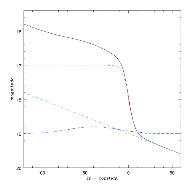
Figure 8: The analytic function used to fit the light curves is shown with the black continuous line. The dashed lines represent the decomposition of the main function in its three addends: the Fermi-Dirac in red, a straight line in green, and a Gaussian function in blue.

The resulting analytic function we use to model the light curves, is the sum of the three functions detailed above

$$\mathcal{F}(t) = f_{FD}(t)+l(t)+g(t)$$ (8)

$$= \frac{-a_{0}}{1+e^{\frac{t-t_{PT}}{w_{0}}}}+p_{0}\,(t-t_{PT})+m_{0}-P\,e^{-\left(\frac{t-Q}{R}\right)^{2}}$$

which has 8 free parameters. It is fitted to the individual light curves using a $\chi^{2}$ minimizing procedure. In order to find the minimum $\chi^{2}$ we use the Downhill Simplex Method (see Appendix 7), which although is not very efficient in terms of the number of iterations required, provides robust solutions. Examples of the analytic fits are shown as dotted lines in Figures 4 and 5. Although we cannot model most of the small scale features in the plateau, the fitting does a really good job modelling the transition. Furthermore, the analytic function gives us important parameters that characterize the light curve shape, particularly $t_{PT}$ which provides a time origin. In the plots in Fig. 4 the time axis is chosen to coincide with the value of this parameter obtained from the $V$ light curve. A critical quantity in the analysis that follows is $t_{PT}$ and its uncertainty, both of which determine the uncertainties in all the relevant SCM quantities. Normally, when the tail phase has been observed the $\chi^{2}$ minimizing routine has no difficulties finding $t_{PT}$ and delivers a credible error. On the other hand, when the light curve does not have any late-time data points the routine underestimates $\sigma(t_{PT})$, in which case we need to provide a more realistic estimate of this uncertainty. The criteria to fix $\sigma(t_{PT})$ depend on what fraction of the transition phase was sampled. Two useful parameters are introduced to describe such sampling:

$t_{f}$ : the day of the last data point for a given SN.

$t_{end}$ : the approximate day of the end of the $V$-band plateau. We estimate this time around each observed point, by calculating the magnitude difference, $\Delta m$, between the previous and the following point. We start from the earliest epochs onward in time, until $\Delta m$ exceeds 0.7 mag. This value is an input parameter for the fitting routine (see Appendix 7).

The criteria to estimate $t_{PT}$ and $\sigma(t_{PT})$ are the following,

1. When the transition can be clearly seen, but if we are uncertain that the last data point (at $t=t_{f}$) belongs to the tail phase, we set a conservative estimate of $\sigma(t_{PT})$=5 days. An example of such a case is SN 2003hl (Fig. 4).

2. When the transition can be clearly seen, but we are sure that the last data point (at $t=t_{f}$) does not belong to the tail phase (see SN 2003hg and SN 2003iq in Fig. 5), the routine usually fails to converge to a reasonable value because there are not enough constraints on the transition phase. We identify the failing cases when $t_{PT}>t_{end}+45$ because $t_{PT}$ is never greater than $t_{end}+25$. In these cases, we set $t_{PT}=t_{end}+15$ since the typical value for the width of the transition is 30 days. For this same reason the value of $\sigma(t_{PT})$ is set to 15 days, a very conservative value as it encompasses the full possible range of $t_{PT}$ values.

3. When the plateau was extensively observed for more than 100 days but could not detect any hints of the transition (see SN 1999br in Fig. 5), we arbitrarily set $t_{PT}=t_{f}+15$, because the plateau phase usually lasts $\sim$100 days. In the two cases where we face this situation, $\sigma(t_{PT})$ is set to 20 days, which generously covers the possibility of a longer plateau.

Regardless of the sampling of the light curves, we assign a minimum of $\sigma(t_{PT})=2$.

The light curve fits also have a healthy benefit: they allow us to interpolate magnitudes at epochs where only one of the magnitudes was obtained and the second magnitude, necessary to construct a color, is missing. Without a color we would be unable to calculate the AKA corrections, so that the interpolation feature is extremely beneficial as it permits one to correct magnitudes at all epochs.

2 Color curves fits

Figure 9 shows the ($B\!-\!V$), ($V$ – $R$), and ($V$ – $I$) colors of three proto-typical Type II-P SNe corrected for $A_{G}$ and $K$-terms.

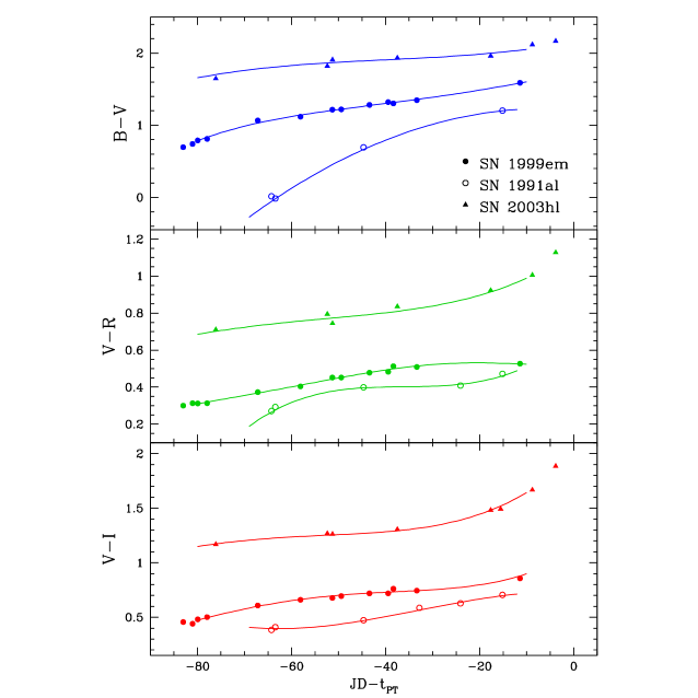
Figure 9: ($B\!-\!V$), ($V$ – $R$), and ($V$ – $I$) color curves of SN 1999em (filled circles), SN 1991al (open circles) and SN 2003hl (filled triangles) corrected for $A_{G}$ and $K$-terms. This comparison demonstrates that each SN displays a different color evolution, which prevents us to determine color excesses from a simple color offset after correcting for $A_{G}$ and $K$-terms.

The time origin (the $x$-axis) corresponds to $t_{PT}$, i.e. the middle of the transition phase. In each case we employ all the data points between day –100 and  –10 to fit a Legendre polynomial shown with solid lines in Fig. 9. The degree of the polynomial was chosen on a case-by-case basis and varied between 3rd and 6th order. It is evident that, during the plateau phase, the photosphere gets redder with time owing to the decrease of the surface temperature as the SN expands. In theory the photospheric temperature should approach and never get below the temperature of hydrogen recombination around 5,000 K. Based on this physical argument, Hamuy & Pinto (2002) argued that all SNe II-P should reach the same intrinsic colors toward the end of the plateau phase and, therefore, they proposed that the color excesses measured at this phase could be attributed to dust reddening in the SN host-galaxy and be exploited to measure $A_{host}$. Hamuy & Pinto (2002) performed their analysis with a simple naked-eye estimate of the asymptotic colors. Here we improve significantly this situation through the formal color curve fitting procedure describe above.

Armed with the polynomial fits we proceeded to interpolate colors on a continuous one-day spaced grid between day –80 and –10 for analyzing colors at multiple epochs (see § 3). In a handful of cases the data did not encompass the whole grid and we had to extrapolate colors, but never by more than 3 days from the nearest data point.

3 Fe 2 based expansion velocity curves

The third ingredient for SCM is the velocity of the SN ejecta. It is well known that different spectroscopic lines yield different expansion velocities. The Fe 2 $\lambda 5169$ line is thought to closely match the SN photospheric velocity and has been usually employed for SCM and EPM. Here we use that line as a proxy for the velocity of the SN ejecta. Due to the expansion of the envelope, the spectral lines show a P-Cygni profile with an emission centered at the rest-frame wavelength $\lambda_{0}$ and an absorption shifted bluewards by $\Delta\lambda$. From a measurement of $\Delta\lambda$ we can compute an expansion velocity

$$\upsilon_{exp}=c\times\frac{\Delta\lambda}{\lambda_{0}}$$ (9)

In this study we use the expansion velocities measured by Jones et al. (2008). Figure 10 shows Fe 2 velocities as a function of SN phase, for four different SNe selected for their wide range of sampling characteristics.

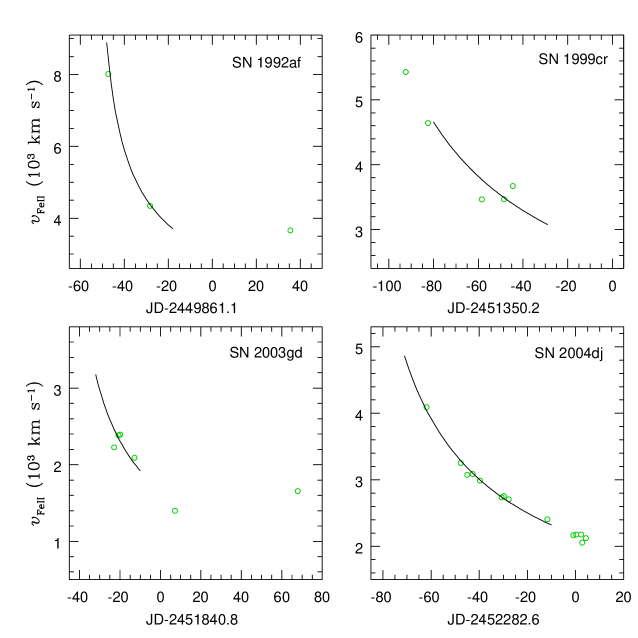
Figure 10: Four expansion velocity curves representative of the SN sample measured by means of the Fe 2 $\lambda$5169 line profile. The solid lines correspond to a power law (eq. 10). For SN 1992af (upper left panel) we fit only two velocities (see § 3 for more details). The upper right panel shows a 15 days extrapolation for SN 1999cr beyond the last data point. The lower left and right panels show a 10 days extrapolation for SN 2003gd and SN 2004dj prior to the first data point.

In all cases the SNe show a systematic decrease of their velocities with time. Two physical arguments support this observational fact: 1) all the shells of the SN undergo an homologous expansion, i.e. the outer shells move faster than the inner shells, and 2) the photosphere recedes in mass allowing us to observe deeper and slower layers of the SN as time passes. As shown by Fig. 10 the Fe 2 $\lambda 5169$ expansion velocity curve during the plateau phase can be properly modeled with a power law of the form

$$\upsilon_{exp}(t)=A\times(t-t_{0})^{\alpha}$$ (10)

where $A$, $t_{0}$ and $\alpha$ are three free fitting parameters without obvious physical meaning.

In general we fit for three free parameters ($A,t_{0},\alpha$), but when only two velocity measurements are available (e.g. SN 1992af in the upper left panel of Fig. 10) we fix the $\alpha$ exponent to –0.5, which corresponds to a typical value for our sample. As shown with solid lines in Figure 10 the fits are quite satisfactory. Here we choose to restrict the power-law fits to the plateau phase, since the power-law behavior is not observed for expansion velocities beyond the transition phase. We use the same one-day continous grid as the color curves in order to interpolate velocities at different epochs between –80 to –10 days. Given the good quality of the fits and the shallow slope at late epochs, we allow extrapolations of up to 15 days past the nearest data point (see SN 1999cr in Fig. 10). At the left boundary we reduce the extrapolations to 10 days prior to the first point, because the power law gets steeper at early times (see SN 2003gd and SN 2004dj in Fig. 10). When only two velocity measurements are available we reduce the extrapolations by 5 days.

3 Host Extinction Determination

While the determination of Galactic reddening is straighforward —thanks to the IR dust maps of Schlegel et al. (1998)—, it is much more challenging to ascertain the extinction due to host-galaxy dust. To address this issue here we assume that, owing to the hydrogen recombination nature of their photospheres, all SNe II-P should evolve from a hot initial stage to one of similar photospheric temperature. If two SNe have similar spectra but suffer different amounts of extinction, all color indices of one object should be redder than the corresponding color indices of the other object. This is the hypothesis we want to test in this section.

Although simple in theory there are a couple of practical difficulties to perform this test. First, it is not always possible to contrain the time of explosion and line up color curves from different objects. One way around this is to use the transition time $t_{PT}$ defined in § 1. The second problem is illustrated in Figure 9: the color curve shapes can vary significantly from SN to SN, preventing one to measure a single color offset between two SNe. Our approach to get around this is to pick a single fiducial epoch in the color evolution and assess the performance of such color as reddening estimator. Our polynomial fits to the color curves are very convenient for this purpose as they allow us to interpolate reliable colors on a day-to-day basis over a wide range of epochs and explore which epoch is the one that gives the best results.

If all SNe share the same intrinsic temperature at some epoch we expect the subset of dereddened SNe to have nearly identical colors ($C_{0}$) and the remaining objects should show color excesses, $E(C)=C-C_{0}$, in direct proportion to their extinctions. A useful diagnostic to check our underlying assumption is the color-color plot. Unreddened SNe should occupy a small region in this plane. If we further assume the same extinction law in the SN host-galaxies, the subset of extinguished objects should describe a straight line originating from such region. The figures of merit in this test are 1) the color dispersion displayed by the unreddened SNe, 2) the slope described by the reddened SNe (which is determined by the extinction law), and 3) the dispersion relative to the straight line (the smaller the better).

We have identified four objects in our sample (SN 2003B, SN 2003bl, SN 2003bn, SN 2003cn) consistent with zero reddening. Such objects were selected for having: 1) no significant Na 1-$D$ interstellar lines in their spectra at the redshifts of their host-galaxies, and 2) dust-free early-time spectra. For the latter we used extinction values determined by Dessart (2008) from fits of Type II-P SN atmosphere models to our early-time spectra. Such models use the SN spectral lines to constrain the photospheric temperature and the continuum to restrict the amount of extinction. As shown in Figure 11, the atmosphere models successfully reproduce the early-time SN spectra.

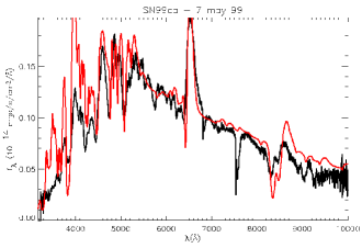
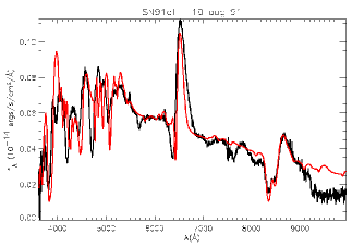
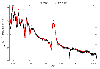
Figure 11: Type II-P SN atmosphere models by Dessart (2008) (red line) fitted to our spectra (black line). The top panel shows an example of an unsatisfactory fit to one of our late-time spectra. The middle panel shows a better fit to an early-time spectrum of SN 1991al. A much better fitting is achieved for an early spectrum of SN 2003bl as shown in the bottom panel.

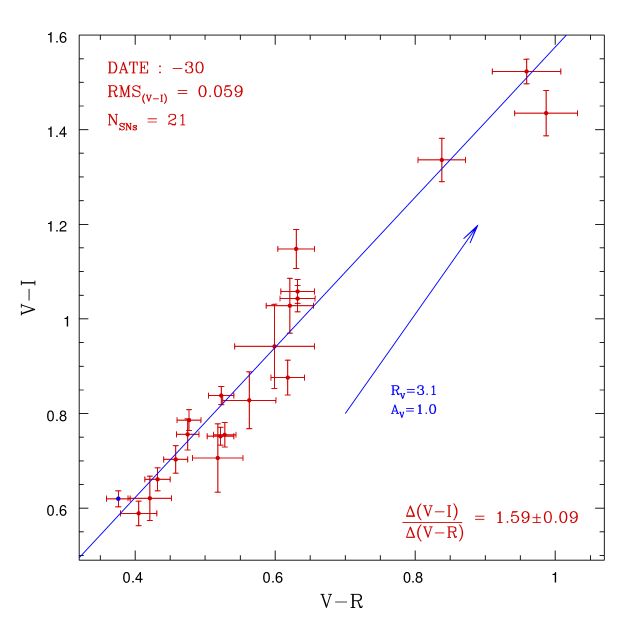
Figure 12: ($V$ – $I$) versus ($V$ – $R$) diagram for 21 SNe II-P having $VRI$ photometry corrected for $A_{G}$ and $K$-terms. The blue line is a least-squares fit to the data, with a slope of $1.59\pm 0.09$. The blue arrow has a slope of 2.12 and corresponds to the reddening vector for a standard Galactic extinction law ($R_{V}=3.1$). With a blue dot is shown the one SN of this subsample consistent with zero extinction having $R$-photometry.

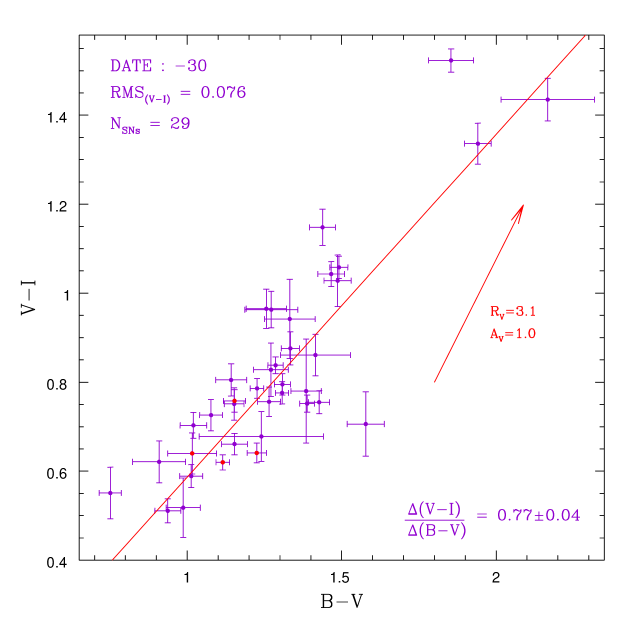
Figure 13: ($V$ – $I$) versus ($B\!-\!V$) diagram for 29 SNe II-P having $BVI$ photometry corrected for $A_{G}$ and $K$-terms. The red line is a least-squares fit to the data, with a slope of $0.77\pm 0.04$. The red arrow has a slope of 1.38 and corresponds to the reddening vector for a standard Galactic extinction law ($R_{V}=3.1$). With red dots are shown the four SNe consistent with zero host-galaxy extinction.

We investigated two color-color plots ($V$ – $I$ versus $V$ – $R$, and $V$ – $I$ versus $B\!-\!V$) over a wide range (from day –50 to –15) of epochs after correcting the photometry for Galactic extinction and $K$-terms. The best results obtained from our scrutiny is the ($V$ – $I$) versus ($V$ – $R$) diagram constructed from day –30 and shown in Figure 12. At this epoch —approximately the end of the plateau— we obtain the linear behavior expected for a sample with the same intrinsic color but different degrees of extinction. Shown with a blue dot is the one SN consistent with zero extinction which is, remarkably, one of the bluest objects in this diagram; the other three unextinguished SNe do not have $R$-photometry. A least-squares fit to the data yields a slope of $1.59\pm 0.09$, which is close but not exactly equal to the $E(V-I)/E(V-R)=2.12$ ratio expected for a Galactic extinction law ($R_{V}=3.1$), shown as a vector in Figure 12. This suggests a somewhat different extinction law in the SN hosts compared to the Galaxy. The dispersion of 0.059 in $V$ – $I$ is a promising result as it translates into an uncertainty of $A_{host}(V)\,=\,0.15$ mag, which corresponds to the limiting precision of this method. The reduced $\chi^{2}$ of 1.55 implies that the dispersion can be accounted almost solely by our error bars and that any instrinsic color dispersion in our sample is $\leq 0.06$. The bottom line is that both the ($V$ – $R$) and ($V$ – $I$) colors fulfill the minimum requirements as reddening indicators.

The best results from the ($B\!-\!V$) versus ($V$ – $I$) analysis were obtained from day –30, which are shown in Figure 13. The four SNe consistent with zero extinction, shown with red dots, average colors $(B-V)_{0}=1.147\pm 0.053$ and $(V-I)_{0}=0.656\pm 0.053$. Note that there are five SNe in this diagram which are slightly bluer than the unreddened sample. The $V$ – $I$ color dispersion of 0.076 is greater than that obtained in Fg. 12 and is most likely due to the $B\!-\!V$ color, since the $B$-band is more sensitive to the metallicity of the SN, owing to several absorption lines that lie in this spectral region. Therefore we believe that the greater dispersion in this diagram could be due to the different metallicities of our SN sample. A least-squares fit to the data yields a slope of $0.77\pm 0.04$. This slope is quite different than the $E(V-I)/E(B-V)=1.38$ ratio expected for the Galactic extinction law (shown as a vector in Figure 13), in agreement with the suggestion made in the previous paragraph from the ($V$ – $I$) versus ($V$ – $R$) diagram.

We conclude from our exploration that, while the $B\!-\!V$ color is problematic, both the ($V$ – $R$) and ($V$ – $I$) colors offer a promising route for dereddening purposes. In what follows we will employ solely the $V$ – $I$ color since only a small subset of our objects possess $R$ photometry. Although the evidence points to a non-Galactic reddening law, for now we will assume a standard reddening law (later on we will relax this assumption; see section 2). Using our library of SNe II spectra we computed synthetically the appropriate conversion factor between $E(V-I)$ and $A_{V}$ for Type II SNe and a standard reddening law ($R_{V}=3.1$), which yielded:

$$\beta_{V}=\frac{A_{V}}{E(V-I)}=2.518$$ (11)

Assuming an intrinsic ($V$ – $I$)${}_{0}=0.656\pm 0.053$ the host-galaxy extinction can be computed, with its corresponding uncertainty, from:

$$A_{V}(V-I) = 2.518\times[(V-I)-0.656]$$ (12)

$$\sigma(A_{V}) = 2.518\times\sqrt{\sigma_{(V-I)}+0.053^{2}+0.059^{2}}$$

Table 1: Host-galaxy extinctions for all 37 SNe

SN name	$A_{V}$(spec)	subclass	$A_{V}$(Na 1-$D$)	$A_{V}$($V$ – $I$)
1991al	0.31(16)	silver	0.31(06)	–0.17(21)
1992af	1.24(31)	coal	0.17(15)	–0.37(21)
1992am	$\cdots$		0.00(43)	0.52(23)
1992ba	0.43(16)	silver	0.00(03)	0.30(21)
1993A	0.00(31)	bronze	0.00(54)	0.06(25)
1999br	0.25(16)	silver	0.00(04)	0.94(25)
1999ca	0.12(31)	coal	0.34(05)	0.25(21)
1999cr	0.47(31)	coal	0.69(21)	0.12(21)
1999em	0.31(16)	gold	1.01(05)	0.24(21)
1999gi	0.56(16)	silver	0.50(08)	1.02(21)
0210	0.31(31)	bronze	0.00(23)	0.31(36)
2002fa	$\cdots$		0.00(14)	–0.35(26)
2002gw	0.40(19)	silver	0.00(02)	0.18(22)
2002hj	0.16(31)	bronze	0.00(06)	0.24(22)
2002hx	0.16(25)	coal	0.00(16)	0.38(22)
2003B∗	0.00(25)	silver	0.12(05)	–0.09(21)
2003E	1.09(31)	coal	0.71(07)	0.78(23)
2003T	0.53(31)	coal	0.19(19)	0.35(21)
2003bl∗	0.00(16)	gold	0.11(10)	0.26(21)
2003bn∗	0.09(16)	silver	0.00(03)	–0.04(21)
2003ci	0.43(31)	coal	0.00(23)	0.78(23)
2003cn∗	0.00(25)	gold	0.00(09)	–0.04(23)
2003cx	0.65(25)	coal	$\cdots$	–0.27(25)
2003ef	1.24(25)	gold	1.40(12)	0.98(21)
2003fb	0.37(31)	coal	0.54(23)	1.24(23)
2003gd	0.40(31)	coal	0.00(04)	0.33(21)
2003hd	0.90(31)	coal	0.74(27)	0.01(21)
2003hg	$\cdots$		2.29(12)	1.97(24)
2003hk	0.65(31)	coal	1.69(20)	0.44(25)
2003hl	1.24(25)	gold	1.84(09)	1.72(23)
2003hn	0.59(25)	coal	0.64(08)	0.46(21)
2003ho	1.24(31)	bronze	1.28(10)	2.19(21)
2003ip	0.40(31)	coal	0.42(08)	0.56(22)
2003iq	0.37(16)	silver	0.91(04)	0.25(22)
2004dj	0.50(25)	coal	0.26(06)	–0.09(23)
2004et	0.00(25)	coal	1.17(02)	0.13(27)
2005cs	$\cdots$		$\cdots$	0.72(30)

where $V$ – $I$ corresponds to the color of a given SN at day –30 (corrected for $K$-terms and foreground extinction) and $\sigma_{(V-I)}$ combines the instrumental errors in the $V$ and $I$ magnitudes, the RMS of the $A_{G}$ and $K$ terms (see § 1 and § 2 respectively), and the uncertainty in $t_{PT}$ (§ 1). The uncertainty in the intrinsic ($V$ – $I$)₀ color was also included in the error of $A_{V}$ along with the ($V$ – $I$) RMS in the ($V$ – $I$) versus ($V$ – $R$) diagram. The host-galaxy reddening values obtained from this technique are listed in column 5 of Table 1 (with the uncertainties given in parenthesis for the whole sample of 37 SNe). There are eight SNe with ($V$ – $I$) colors bluer than ($V$ – $I$)₀ which stand out in this table for their negative reddenings. Although not physically meaningful, these negative values are statistically consistent with zero or moderate reddenings. In fact, seven out of these eight objects differ by $<1.1\sigma$ from zero reddening. Only SN 1992af differs by $1.8\sigma$ from $A_{host}=0$. In the following section we compare this method to other dereddening techniques.

Chapter 3 Analysis

1 Comparing dereddening techniques

At our request, Dessart (2008) has kindly performed fits of SNe II-P atmosphere models to our library of spectra. In these fits the spectral lines are used to constrain the photospheric temperature and the corresponding continuum is employed to estimate the extinction. A crucial condition for this technique to work is the spectrophotometric quality of the spectra.

In general our observations were obtained with the slit oriented along the paralactic angle and the relative shape of the spectra should be accurate. However, this was not always possible and sometimes the spectra were contaminated from light of the host-galaxy or the slit could not be rotated. For all these reasons we first checked the flux calibration of each spectrum by synthesizing magnitudes and comparing them to the observed magnitudes, duly interpolated to the time of the spectroscopy. In general we found good agreement between the observed and synthetic colors (Figure 1), thus confirming our confidence in the flux calibration.

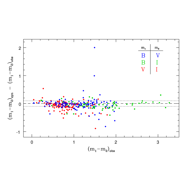
Figure 1: Synthetic colors minus observed colors versus observed colors for the 150 library spectra. The 64 cases (18% of all cases) with colors outside the $\sigma=0.1$ contours are selected for a “mangling” correction, whose purpose is to correct the flux calibration of a spectrum and make it consistent with the observed photometry.

In the 64 cases (18% of all cases) where we found significant differences between synthetic and observed colors ($\geq$ 0.1 for any color) we applied a low-order polynomial correction to the spectrum. Basically, this “mangling” correction used the observed photometry to change the slope of a spectrum. After checking the flux calibration (and mangling it, if needed) the next step was to correct for Galactic absorption and de-redshift the spectra. This database was then used by Dessart (2008) for the atmosphere model fits. Examples of the fits are shown in Fig. 11.

The resulting spectroscopic reddenings are summarized in column 2 of Table 1. As pointed out by Dessart (2008), the spectrum fitting technique works much better with early-time spectra than with late-time observations. At late times the photosphere has receded in mass exposing inner and more metal-rich layers, which translates into an over-abundance of heavy-elements absorption lines. Therefore the fitting to the continuum —practically a temperature fitting— is hampered by the presence of strong absorption lines at late times. According to this we divided our sample in four quality subcategories based on the epoch and the flux quality of the spectra used in the reddening determination:

                 $\diamond$ 

gold : early-time spectra, without mangling correction

                 $\diamond$ 

silver : early-time spectra, with mangling correction

                 $\diamond$ 

bronze : late-time spectra, without mangling correction

                 $\diamond$ 

coal : late-time spectra, with mangling correction

Note that the main criterion is whether the spectrum is early or late and the second criterion corresponds to the flux calibration quality. We trust more the spectra that do not require any corrections as they reflect that the observations were better performed, so we consider the unmangled spectra as higher-quality than the mangled ones. This sub-classification is given for each SN in column 3 of Table 1. As the reader can notice, the error is directly related to this sub-classification. Dessart (2008) assigns an error of $\sigma_{E(B-V)}=0.05$ when using early-time spectra, and $\sigma_{E(B-V)}=0.1$ when using late-time spectra. We refine this argument ramping up from 0.05 to 0.10, depending on the number of spectra employed for each extinction determination. These values are given in Table 1 in units of $A_{V}=3.1\times E(B-V)$.

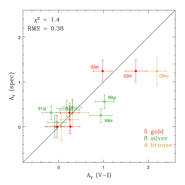
Figure 2: Comparison between two dereddening techniques: the spectrum fitting method ($y$-axis, Dessart 2008) and our technique ($x$-axis, § 3). The figure shows three subclasses defined by the quality of the spectroscopic data used by Dessart (2008): the gold+silver+bronze sample (see § 1). The solid black line is the one-to-one relation.

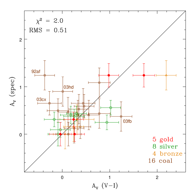
Figure 3: Comparison between two dereddening techniques: the spectrum fitting method ($y$-axis, Dessart 2008) and our technique ($x$-axis, § 3). The figure shows the same three subclasses as Fig. 2 plus the worst quality coal sample (see § 1). The solid black line is the one-to-one relation.

Figure 2 shows a comparison between the spectroscopic reddenings $A_{V}$(spec) and our color reddenings $A_{V}(V-I)$ derived in § 3, for the 17 SNe belonging to the top three subclasses (gold+silver+bronze). A good agreement is displayed between both techniques with a dispersion of 0.38 mag. The resulting $\chi^{2}=1.4$ suggests that this dispersion is consistent with the combined errors between both techniques. The exceptions are two objects: SN 1999br and SN 2003ho. The first object (SN 1999br) only has plateau photometry making hard the determination of $t_{PT}$. Although the error in $t_{PT}$ is quite large (20 days), this uncertainty does not have a great impact on the error of the $V$ – $I$ color due to the flatness of the color curve at these epochs (+0.0024 per day). Another cause for the disagreement is the extreme properties (low luminosity and velocity) of this SN which might also have a $V$ – $I$ color instrinsically redder than that of the bulk of the SNe. The second discrepant object (SN 2003ho) belongs to the bronze group so it is possible that the difference could be due to the use of a late-time of the spectrum in the determination of the spectroscopic reddening.

Figure 3 shows the same comparison, but this time we include the 16 lowest-quality coal SNe. This inclusion clearly deteriorates the good agreement seen in Fig. 2 from $\sigma=0.38$ mag to $\sigma=0.51$ mag ($\chi^{2}=2.0$), namely due to SN 1992af, SN 2003cx, SN 2003hd, and SN 2003fb. This confirms the warning by Dessart (2008), namely, that his spectroscopic technique works much better with early-time spectra. The large value of $\chi^{2}$ also suggests that the errors in the spectroscopic reddenings derived from late-time spectra are underestimated.

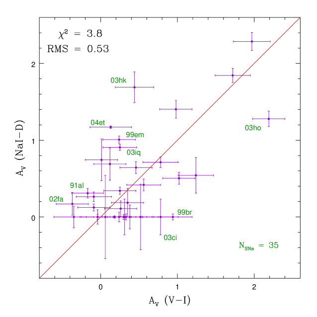
Figure 4: Comparison between two dereddening techniques: the Na 1-$D$ interstellar line ($y$-axis) and our technique ($x$-axis, § 3). The equivalent width of the Na 1-$D$ interstellar line are transformed into visual extinctions according to the calibration given by Barbon et al. (1990).

Another way to estimate host-galaxy reddening is from the Na 1-$D$ $\lambda\lambda$5893,5896 interstellar absorption doublet observed in the SN spectrum at the host-galaxy redshift. Whenever the line was detected we measured its equivalent width; in those cases where we did not detect the Na 1-$D$ line we assigned it a null value. In all cases we estimated the uncertainty in the equivalent width ($EW$) based on the signal-to-noise of the continuum around this line. We converted these measurements into visual extinctions $A_{V}$(Na 1-$D$) using the calibration of Barbon et al. (1990):

$$E(B-V)\,\simeq\,0.25\,\times\,EW(\mbox{{Na {1}}-$D$}),$$ (1)

and tabulate our results in column 4 of Table 1. The comparison between $A_{V}$(Na 1-$D$) and our technique, shown in Figure 4, exhibits a dispersion of 0.53 mag ($\chi^{2}=3.8$), which is much higher than the $\sigma$=0.38 mag obtained from the previous comparison. The disagreement can be attributed to the fact that the absorption line traces the gas content along the line of sight, but does not necessarily probe dust (Munari & Zwitter 1997). Furthermore, reddenings derived from the EW of the Na 1-$D$ lines measured from low-dispersion spectra simply cannot be expected to be precise which is exactly our case. The basic problem is that the D lines produced by a typical interstellar cloud are saturated (Hobbs 1974). The only way that one can hope to derive the reddening from the D lines is via very high-dispersion spectra that resolve the lines and allow the column density to be derived.

2 The Luminosity-Expansion Velocity relation

Armed with the dereddening method based on late-time colors we can now revisit the $LEV$ relation originally discovered by Hamuy & Pinto (2002) which is at the core of the SCM. For this purpose we applied AKA corrections (§ 1) to our photometry, we used our analytic fits (§ 1) to interpolate $BVI$ magnitudes on day –30, and we employed the CMB redshifts in Table 1 to convert apparent magnitudes to absolute values (assuming $H_{0}=70$ km s^-1 Mpc^-1). The expansion velocities were determined from the minimum of the Fe 2 $\lambda$5169 P-Cygni line profiles. We performed a power-law fit to interpolate a velocity contemporaneous to the photometry (day –30) as described in section 1. From our original sample of 37 SNe II-P we were able to use 30 SNe to build this relation, since five of them do not have Fe 2 velocities at day –30, and two others have extremely low redshifts ($cz_{CMB}<300$ km s^-1).

Figure 5 shows the resulting $LEV$ relation (absolute magnitude versus expansion velocity) for all $BVI$ bands. Evidently we recover the result of Hamuy & Pinto (2002), namely that the most luminous SNe have greater expansion velocities. In their case the data were modeled with a linear function. Our sample suggests that the relation may be quadratic, but we need more SNe at low expansion velocities to confirm this suspicion. Linear least-squares fits to our $BVI$ data yields the following solutions

$$M_{abs}(B) = 3.50(\pm 0.30)~{}\log{(\upsilon_{\mbox{\scriptsize FeII}}/5000)}-16.01(\pm 0.20)$$ (2)

$$M_{abs}(V) = 3.08(\pm 0.25)~{}\log{(\upsilon_{\mbox{\scriptsize FeII}}/5000)}-17.06(\pm 0.14)$$ (3)

$$M_{abs}(I) = 2.62(\pm 0.21)~{}\log{(\upsilon_{\mbox{\scriptsize FeII}}/5000)}-17.61(\pm 0.10)$$ (4)

which are shown with solid lines in Figure 5.

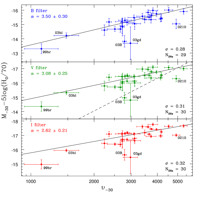
Figure 5: $BVI$ band absolute magnitudes ($y$-axis) against the Fe 2 expansion velocity ($x$-axis) for 29–30 SNe. We use the magnitudes corrected for Galactic extinction, $K$-terms, and host-galaxy extinction together with a value of the Hubble constant of 70 km s^-1 Mpc^-1. The dashed line in the middle panel represents the $LEV$ relation for the $V$-band found by Hamuy & Pinto (2002) obtained from magnitudes and velocities measured at day 50 past the explosion (approximately day –60 in our own time scale).

The relation found by Hamuy & Pinto (2002) for the $V$-band is shown with the dashed line in the middle panel of the same figure. Given that the study of Hamuy & Pinto (2002) was performed using data at day 50 after the explosion (around day –60 in our time scale), it is not unexpected that their $LEV$ relation is shifted to higher expansion velocities. Some of the difference in slope is explained by the inclusion of SN 2003bl in our sample, which flattens the correlation. This relation exhibits a dispersion of 0.3 mag, similar to that reported before. This low scatter is very encouraging as it implies that the expansion velocities can be used to predict the SN luminosities, to standardize them, and to derive distances.

3 Hubble diagrams

The $LEV$ relation shown in the previous section implies that a spectroscopic measurement of the expansion velocity of a SN II-P can be used to compute a corrected luminosity which should be approximately the same for all SNe. We examine the reality of this property of SNe II-P in the magnitude-redshift Hubble diagram. For this purpose we employ Fe 2 velocities (in units of km s^-1), $BVI$ apparent magnitudes corrected for $K$-terms, Galactic reddening, and host-galaxy reddening determined from $V$ – $I$ colors, and host-galaxy redshifts in the CMB frame. Table 1 lists these values for the 37 SNe of our sample, of which 35 meet the requirement of being in the Hubble flow ($cz_{CMB}>300$ km s^-1). A perfect distance indicator would describe a straight line in the Hubble diagram, so the figure of merit to assess the performance of this method is the dispersion from the fit. Along this section we use dispersions weighted by the errors to evaluate the precision of the Hubble diagrams.

Table 1: Magnitudes, expansion velocities, and $V$ – $I$ colors for day –30

SN name	$cz_{CMB}$∗	$B$	$V$	$I$	$\upsilon_{\mbox{\scriptsize FeII}}$	$V$ – $I$
1991al	4480	17.944(036)	16.917(029)	16.333(020)	5328(202)	0.589(022)
1992af	5359	18.024(038)	17.096(029)	16.706(053)	4529(212)	0.511(027)
1992am	14007	20.443(117)	19.053(038)	18.218(033)	$\cdots$	0.830(046)
1992ba	1245	16.962(040)	15.657(031)	14.886(022)	2237(068)	0.776(021)
1993A	8907	20.636(127)	19.309(089)	18.657(057)	$\cdots$	0.678(047)
1999br	1285	19.010(022)	17.582(013)	16.574(008)	1127(205)	1.028(011)
1999ca	3108	17.901(071)	16.489(055)	15.735(034)	$\cdots$	0.755(025)
1999cr	6363	19.435(067)	18.418(051)	17.723(035)	3095(207)	0.703(025)
1999em	670	15.331(034)	13.998(023)	13.245(017)	2727(056)	0.752(019)
1999gi	831	16.554(032)	15.060(019)	14.011(022)	2725(061)	1.058(025)
0210	15082	21.955(044)	20.572(028)	19.733(035)	4923(206)	0.780(110)
2002fa	17847	21.222(072)	20.243(052)	19.709(088)	4176(061)	0.518(065)
2002gw	2878	18.575(020)	17.491(029)	16.752(014)	2669(063)	0.726(035)
2002hj	6869	19.705(084)	18.582(061)	17.939(042)	3657(065)	0.751(031)
2002hx	9573	20.328(056)	19.164(035)	18.360(028)	3960(203)	0.805(031)
2003B	1105	17.078(022)	15.966(018)	15.341(015)	2795(067)	0.620(017)
2003E	4380	19.659(046)	18.368(026)	17.472(024)	2869(203)	0.965(024)
2003T	8662	20.541(028)	19.227(020)	18.423(022)	2803(203)	0.795(024)
2003bl	4652	20.158(042)	18.961(020)	18.230(019)	1475(202)	0.758(025)
2003bn	4173	18.638(045)	17.403(034)	16.769(024)	2719(202)	0.641(020)
2003ci	9468	$\cdots$	19.634(035)	18.648(029)	2876(077)	0.963(034)
2003cn	5753	19.852(024)	18.827(015)	18.182(014)	2510(207)	0.640(017)
2003cx	11282	20.417(100)	19.513(050)	19.050(067)	3734(205)	0.551(058)
2003ef	4504	19.304(032)	17.837(024)	16.792(017)	$\cdots$	1.043(015)
2003fb	4996	20.521(122)	19.085(092)	17.940(056)	3120(206)	1.148(040)
2003gd	359	15.208(045)	13.965(036)	13.167(023)	2976(230)	0.786(019)
2003hd	11595	20.462(031)	19.320(014)	18.658(018)	3741(069)	0.661(022)
2003hg	3921	20.247(091)	18.067(040)	16.603(025)	3398(211)	1.435(027)
2003hk	6568	19.478(036)	18.201(024)	17.380(023)	3618(087)	0.828(026)
2003hl	2198	19.124(062)	17.219(038)	15.806(027)	2354(063)	1.336(027)
2003hn	1102	16.416(020)	15.153(011)	14.307(015)	3121(074)	0.836(018)
2003ho	4134	20.779(084)	18.946(026)	17.419(016)	4152(080)	1.523(022)
2003ip	5050	18.894(046)	17.549(035)	16.664(025)	3813(204)	0.876(021)
2003iq	2198	17.396(049)	16.124(037)	15.362(024)	3482(063)	0.756(018)
2004dj	180	12.973(074)	12.046(035)	11.416(033)	2725(202)	0.621(043)
2004et	–133	13.683(220)	12.099(171)	11.378(104)	2901(202)	0.707(070)
2005cs	635	16.099(062)	14.749(051)	13.824(055)	$\cdots$	0.957(067)

1 Using $A_{V}$( $V$ – $I$) and $A_{V}$(spec)

The top left panel of Figure 6 shows a Hubble diagram constructed from $B$-band magnitudes interpolated to day –30 previously corrected for Galactic extinctions and $K$-terms. The top right panel shows magnitudes additionally corrected for the $LEV$ relation, the bottom left panel includes further corrections for host-galaxy extinction (using the $V$ – $I$ color calibration given in section 3). In each case we perform a linear least-squares fit of the form,

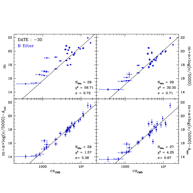
Figure 6: $B$-band Hubble diagrams. The top panel shows magnitudes interpolated to day $-30$ previously corrected for Galactic extinction and $K$-terms; the top right panel shows magnitude additionally corrected for expansion velocities; the bottom left panel includes further corrections for color-based host-galaxy extinction (using the $V$ – $I$ color calibration given in section 3); the bottom right panel replaces the color-based extinction for the spectroscopic reddenings of Dessart (2008).

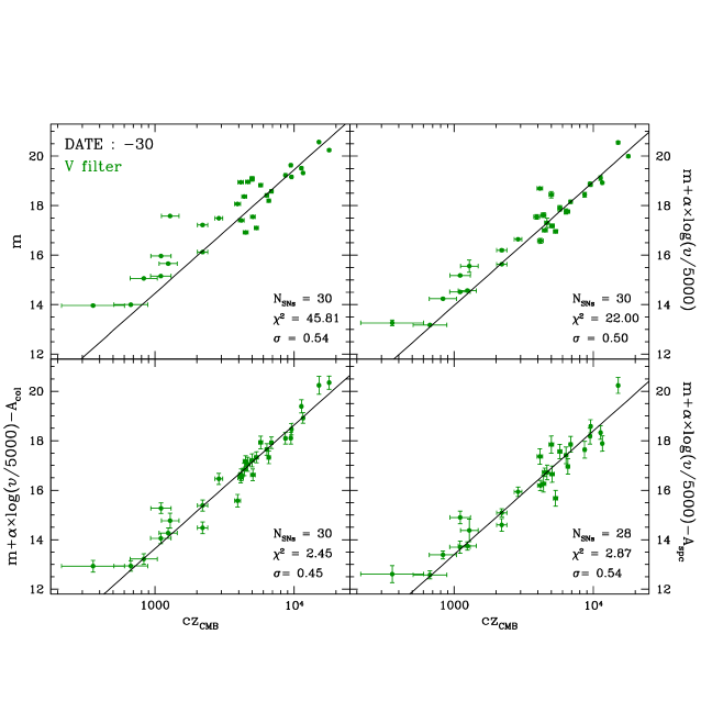
Figure 7: $V$-band Hubble diagrams. The top panel shows magnitudes interpolated to day –30 previously corrected for Galactic extinction and $K$-terms; the top right panel shows magnitude additionally corrected for expansion velocities; the bottom left panel includes further corrections for color-based host-galaxy extinction (using the $V$ – $I$ color calibration given in section 3); the bottom right panel replaces the color-based extinction for the spectroscopic reddenings of Dessart (2008).

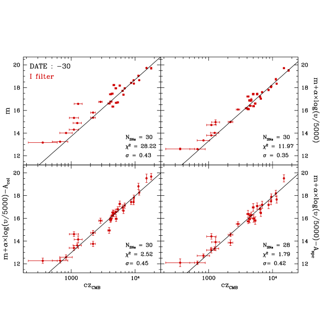
Figure 8: $I$-band Hubble diagrams. The top panel shows magnitudes interpolated to day $-30$ previously corrected for Galactic extinction and $K$-terms; the top right panel shows magnitude additionally corrected for expansion velocities; the bottom left panel includes further corrections for color-based host-galaxy extinction (using the $V$ – $I$ color calibration given in section 3); the bottom right panel replaces the color-based extinction for the spectroscopic reddenings of Dessart (2008).

$$m~{}+~{}\alpha\,\log{(\upsilon_{\mbox{\scriptsize FeII}}/5000)}~{}-~{}A_{host}~{}=~{}5\,\log{cz}~{}+~{}zp$$ (5)

where $m$ is the apparent magnitude corrected for $K$-terms and Galactic absorption, $\upsilon_{FeII}$ is the expansion velocity, $A_{host}$ is the host-galaxy absorption, and $z$ is the CMB redshift. The only fitting parameters are $\alpha$ and $zp$; in the top left panel we set $\alpha=0$ and we only fit for the zero point.

The dramatic decrease in the dispersion, from 0.72 to 0.36 mag clearly demonstrates the benefitial effects of adding the velocity and host-galaxy extinction terms. An inspection of the $V$-band diagram (Fig. 7) shows a large scatter of 0.54 mag in the top left panel. When we correct for expansion velocities, the scatter drops to 0.50 mag. This is certainly not unexpected given the $LEV$ relation reported in the previous section. It is encouraging to notice that the dispersion drops from 0.50 to 0.45 mag when we include our host-galaxy extinction corrections. This indicates the usefulness of our color-based dereddening technique. The reduced $\chi^{2}$ value of 2.45 implies that most of the scatter is accounted by the observational errors. We performed the same analysis using other epochs and we found that day –30 yielded the lowest dispersion. This is also the day for which we reach the maximum number of SNe in our HDs, i.e. moving backwards or forwards in time means losing SNe data (velocity or magnitudes out of the observation range).

If we turn our attention to the $I$-band (Figure 8) the final dispersion is 0.45 mag, identical to that found in the $V$-band. It seems that the dispersion could have some dependence on wavelength, since it decreases from 0.45 in $VI$ to 0.36 mag in $B$. However, it may be due to a sampling effect, because the $VI$ diagrams have one SN more than the $B$ diagram. The scatter of $\sim$ 0.4 mag in $BVI$ is comparable but somewhat larger than the $\sim$ 0.34 dispersion obtained in previous SCM studies (Hamuy & Pinto 2002; Hamuy 2003). It is important to notice that the dispersions are independent of the intrinsic ($V$ – $I$)₀ color calculated in section 3.

In the bottom right panels of Figs. 6, 7, and 8 we examine the SCM using the spectroscopic reddenings determined by Dessart (2008) for a set of 28 SNe II-P (Table 1) instead of our color-based extinctions. The resulting dispersions in $BVI$ are (0.67, 0.54, 0.42), which compare to (0.36, 0.45, 0.45) when using color-based extinctions. All the fitting parameters derived from both dereddening techniques are compiled in Table 2.

2 Leaving $R_{V}$ as a free parameter

The previous analysis suggests that the dispersions are somewhat larger than the observational errors. One possible source of scatter could be the reddening law. As shown in § 3 and Fig. 12 we have evidence pointing toward a somewhat different extinction law in the SN hosts compared to the Galaxy. Here we take this idea a step further and we analyze the Hubble diagram leaving $R_{V}$ as a free parameter. To accomplish this we model the data with the following expression

$$m+\alpha\,\log{(\upsilon_{\mbox{\scriptsize FeII}}/5000)}-\beta(\mbox{$V$\,--\,$I$})~{}=~{}5\,\log{cz}+zp$$ (6)

Note that we are replacing $A_{host}$ in equation 5 with the term $\beta$($V$ – $I$). The $\beta$ factor is a new free parameter to be marginalized along with $\alpha$ and $zp$, and $V$ – $I$ is the color on day –30 corrected for $K$-terms, Galactic extinction but uncorrected for host-galaxy dust. Once $\beta$ is known we can used it to solve for host-galaxy extinction from $A(\lambda)=\beta\,\Bigl{[}\,$($V$ – $I$)$-0.656\,\Bigr{]}$, where 0.656 is the intrinsic $V$ – $I$ color of SNe II-P (see equations 11 and 12 in § 3).

Figure 9 shows the $BVI$ Hubble diagrams for our set of 30 SNe II-P. We get dispersions of (0.28, 0.31, 0.32) in $BVI$ respectively, which compare to (0.36, 0.45, 0.45) when $R_{V}$ is kept fixed. The increase in $\chi^{2}$ is due to the fact that we are not using the intrinsic color, which gives the major contribution to the errors. Although we expect a reduction in the scatter due to the inclusion of an additional parameter, the large drop in the dispersion is remarkable. The last three lines of Table 2 shows the parameters we obtain by minimizing the dispersion in the HD for each band. When we restrict the sample to objects with $cz_{CMB}>3000$ km s^-1(leaving aside SNe with potentially greater peculiar velocities), we end up with 19 SNe in the $B$-band and 20 SNe in the $VI$ bands. The resulting HDs in $BVI$ show dispersions of (0.25, 0.28, 0.30), respectively. Not surprisingly these are lower than the (0.28, 0.31, 0.32) dispersions obtained from the whole sample, and the Hubble constant shows only a mild increase of 3%.

By definition the term $\beta$($V$ – $I$) in equation 6 corresponds to the extinction in a broad-band magnitude (with central wavelenth $\lambda$). Thus, $\beta$ is the ratio $A(\lambda)/E(V-I)$ (see eq. 11 in § 3) and is related to the shape of the extinction law. For each of the $BVI$ bands we used our library of SNe II spectra to compute synthetically the value of $\beta_{\lambda}$ as a function of $R_{V}=A_{V}/E(B-V)$ (see Figure 10). This allowed us to convert the $\beta_{\lambda}$ values resulting from our fits into $R_{V}$ values. Our fits yield $\beta_{\lambda}=(2.67\pm 0.13,1.67\pm 0.10,0.60\pm 0.09)$ for the $BVI$ bands, which translate into $R_{V}=(1.38^{+0.27}_{-0.24},1.44^{+0.13}_{-0.14},1.36^{+0.11}_{-0.12})$. These values are remarkably consistent to each other and significantly lower than the $R_{V}=3.1$ value of the standard reddening law. Independent evidence for a low $R_{V}$ law has been already reported from studies of SNe Ia (see § 4).

The dispersion of 0.28–0.32 mag in the HDs translates into an accuracy of 13–14% in the determination of distances. Although not as good as the $\sim$ 7%–10% precision of SNe Ia (Phillips 1993; Hamuy et al. 1996; Phillips et al. 1999), this is a very encouraging result which demonstrates that SNe II-P have great potential to determine extra-galactic distances, and therefore, cosmological parameters.

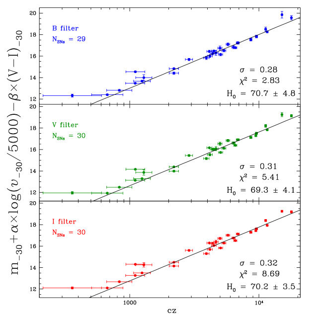
Figure 9: $BVI$ Hubble diagrams leaving $R_{V}$ as a free parameter.

Table 2: Fitting parameters from the Hubble diagrams

Reddening
estimator	filter	$\alpha$	$\beta$	$zp$
($V$ – $I$)	$B$	3.27$\,\pm\,$0.37	$\cdots$	–0.24$\,\pm\,$0.08
	$V$	3.01$\,\pm\,$0.36	$\cdots$	–1.36$\,\pm\,$0.08
	$I$	2.99$\,\pm\,$0.36	$\cdots$	–2.02$\,\pm\,$0.08
spectral	$B$	4.77$\,\pm\,$0.47	$\cdots$	–0.60$\,\pm\,$0.11
analisis	$V$	4.22$\,\pm\,$0.45	$\cdots$	–1.60$\,\pm\,$0.10
	$I$	3.67$\,\pm\,$0.43	$\cdots$	–2.11$\,\pm\,$0.10
($V$ – $I$) +	$B$	3.50$\,\pm\,$0.30	2.67$\,\pm\,$0.13	–1.99$\,\pm\,$0.11
variable $R_{V}$	$V$	3.08$\,\pm\,$0.25	1.67$\,\pm\,$0.10	–2.38$\,\pm\,$0.09
	$I$	2.62$\,\pm\,$0.21	0.60$\,\pm\,$0.09	–2.23$\,\pm\,$0.07

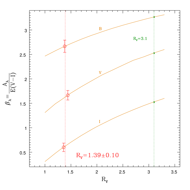
Figure 10: $R_{V}$ versus $\beta$. The solid lines are computed from our library of SNe II spectra for each of the $BVI$ bands. The $\beta$ parameters derived from the HDs in Figure 9 are shown with red open circles for each of the $BVI$ bands. The red dotted line shows the $R_{V}$ weighted mean for the $BVI$ values of $\beta$. The values for the standard Galactic extinction law are also shown with green dots.

4 The Hubble constant

The Hubble constant is a parameter of central importance in cosmology which can be determined from our Hubble diagrams. This can be accomplished as long as we can convert apparent magnitudes into distances. This calibration was done with two objects for which we found Cepheid distances in the literature: SN 1999em ($\mu=30.34\pm 0.19$; Leonard et al. 2002) and SN 2004dj ($\mu=27.48\pm 0.24$; Freedman et al. 2001). For each calibrating SN we can solve for $H_{0}$ using the following expression

$$\log\,H_{0}~{}=~{}0.2\times\Bigl{[}\,m+\alpha\,\log{(\upsilon_{\mbox{\scriptsize FeII}}/5000)}-\beta(\mbox{$V$\,--\,$I$})-\mu-zp+25\,\Bigr{]}$$ (7)

In this equation $m$ is the apparent magnitude corrected for Galactic absorption and $K$-terms, $\upsilon_{FeII}$ is the expansion velocity, and $V$ – $I$ is the color of the calibrating SN, all measured on day –30 and given in Table 1; $\alpha$, $\beta$, and $zp$ are the fitting parameters given in the bottom three lines of Table 2.

Table 3 summarizes our calculations for the two calibrators. This table shows that the corrected $BVI$ absolute magnitudes of SN 1999em and SN 2004dj differ from each other by 0.86–1.13 mag. This is somewhat greater than the scatter of 0.3 mag in the $LEV$ relation, but statistically plausible. This can be seen in Figure 11 where we plot with red dots the corrected absolute magnitudes of the two calibrating SNe, on top of the whole sample of SNe employed in the HDs (black dots). This difference leads to $H_{0}$ values in the range 62–105 km s^-1 Mpc^-1. A weighted average of the values of Table 3 yields a Hubble constant

$$H_{0}\ =\ 70\ \pm\ 8\quad\mbox{km~{}s${}^{-1}$~{}Mpc${}^{-1}$}$$ (8)

This value compares very well with that derived by Freedman et al. (2001) from SNe Ia ($71\pm 2$ km s^-1 Mpc^-1), and reasonable well with that found by Sandage et al. (2006) ($62.3\pm 1.3$ km s^-1 Mpc^-1) with a similar Type Ia sample. With only two calibrating SNe the SCM still has plenty of room to deliver a more precise value for $H_{0}$.

Table 3: $H_{0}$ calculations

	$M+\alpha\log(\upsilon/5000)-\beta(V-I)$
SN	$B$	$V$	$I$	$H_{0}(B)$		$H_{0}(V)$		$H_{0}(I)$
1999em	–17.94$\,\pm\,$0.20	–18.41$\,\pm\,$0.20	–18.24$\,\pm\,$0.19	64.7$\,\pm\,$	6.8	62.2$\,\pm\,$	6.1	62.9$\,\pm\,$	6.0
2004dj	–17.08$\,\pm\,$0.30	–17.28$\,\pm\,$0.27	–17.13$\,\pm\,$0.26	95.7$\,\pm\,$	14.0	104.5$\,\pm\,$	13.7	104.8$\,\pm\,$	12.9
Average	–17.67$\,\pm\,$0.39	–18.02$\,\pm\,$0.53	–17.84$\,\pm\,$0.53	71$\,\pm\,$	12	69$\,\pm\,$	16	70$\,\pm\,$	16

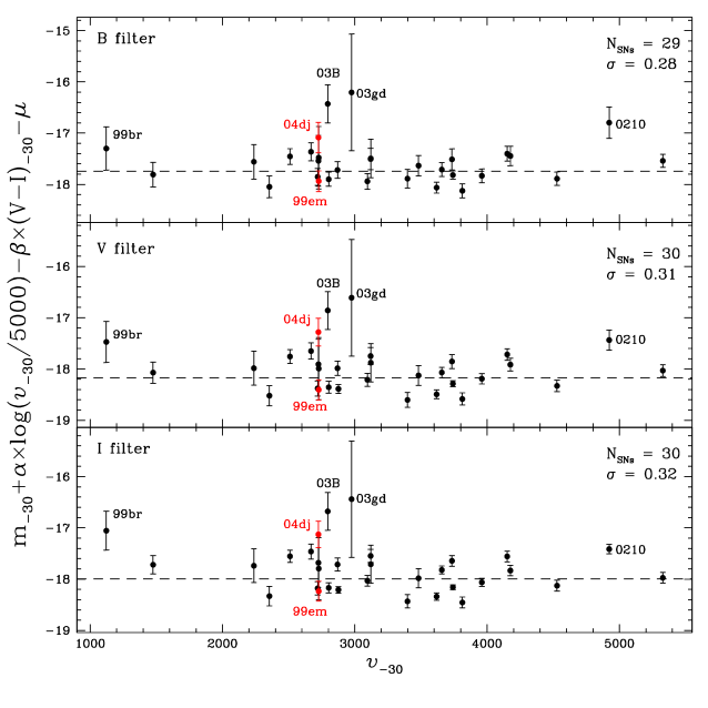
Figure 11: $BVI$ corrected absolute magnitudes ($y$-axis) against the Fe 2 expansion velocity ($x$-axis) for 29–30 SNe (black dots). We use the $H_{0}$ values of Table 3 and the CMB redshifts to compute the distance moduli. The dashed lines show the mean corrected absolute magnitude for the black dots. The red dots are the two calibrating SNe, whose corrected absolute magnitudes were calculated using their Cepheid distances (see Table 3). Note that, as expected, the two calibrating SNe fall on each side of the corrected absolute magnitude distributions.

5 Distances

Armed with standardized absolute magnitudes for SNe II-P, we are in a position to calculate distances to all the SNe of our sample. This can be done with the following expression

$$\mu=m+\alpha\,\log{(\upsilon_{\mbox{\scriptsize FeII}}/5000)}-\beta(\mbox{$V$\,--\,$I$})-\langle M_{corr}\rangle$$ (9)

where $\langle M_{corr}\rangle$ is the weighted mean of the corrected absolute magnitudes of the two calibrating SNe given in Table 3. The resulting values are given in Table 4 for the 37 SNe II-P. The last column of the table shows the weighted averages of their distance moduli.

As mentioned in the introduction, we can evaluate the precision of the SCM from a comparison with EPM distances. For this purpose we employ EPM distances recently calculated by Jones et al. (2008) which are summarized in Table 5 along with our distances for the 11 objects in common between SCM and EPM. Jones et al. (2008) determine EPM distances with two different sets of atmosphere models. The EPM distances determined using the models of Eastman et al. (1996) (E96; column 2) are 12%$\,\pm\,$5% shorter than our SCM distances. On the other hand, the EPM distances determined using the models of Dessart & Hillier (2005) (D05; column 3) are 40%$\,\pm\,$10% greater than our SCM distances. These shifts are calculated weighting by the error in the EPM and SCM distances. These systematic differences can be clearly seen in the upper panel of Figure 12, and more clearly in the fractional differences $(d_{EPM}-d_{SCM})/d_{SCM}$ plotted in the bottom panel.

The systematic differences among the two sets of EPM distances can be solely attributed to the atmosphere models of E96 and D05. New radiative transfer models of SNe II-P are necessary to understand the origin of this discrepancy. Besides the systematic errors in both EPM implementations, we can get an understanding of the internal precision of EPM and SCM after removing the systematic differences and bringing all distances to a common scale. For this purpose we correct the EPM distances to the SCM distance scale by removing the percentage shifts of 1.40 and 0.88. The comparison is shown in Figure 13. The distance differences have dispersions of $\sim$ 13% and $\sim$ 16% using D05 and E96 respectively. This implies that either SCM or EPM produce relative distances with an internal precision between 13–16%. This agrees with the dispersions of 0.25–0.30 mag seen in the HDs restricted to SNe with $cz_{CMB}>300$ km s^-1.

Table 4: Distance Moduli

SN name	Host Galaxy	$\mu_{B}$	$\mu_{V}$	$\mu_{I}$	$\langle\mu\rangle$
1991al	LEDA 140858	34.14(41)	34.04(54)	33.89(53)	34.05(28)
1992af	ESO 340–G038	34.18(41)	34.13(54)	34.13(54)	34.15(28)
1992am	MCG–01–04–039	$\cdots$	$\cdots$	$\cdots$	$\cdots$
1992ba	NGC 2082	31.34(40)	31.31(54)	31.34(53)	31.33(28)
1993A	[MH93a]073838.4	$\cdots$	$\cdots$	$\cdots$	$\cdots$
1999br	NGC 4900	31.67(48)	31.89(59)	32.10(57)	31.86(31)
1999ca	NGC 3120	$\cdots$	$\cdots$	$\cdots$	$\cdots$
1999cr	ESO 576–G034	34.50(42)	34.63(55)	34.59(54)	34.56(28)
1999em	NGC 1637	30.07(40)	29.96(54)	29.94(53)	30.00(28)
1999gi	NGC 3184	30.48(40)	30.51(54)	30.52(53)	30.50(28)
0210	MCG +00–03–054	37.52(50)	37.27(57)	37.09(54)	37.31(31)
2002fa	NEAT J205221.51	37.23(44)	37.16(55)	37.03(54)	37.16(29)
2002gw	NGC 922	33.35(41)	33.46(54)	33.44(53)	33.41(28)
2002hj	NPM1G+04.0097	34.90(41)	34.93(54)	34.97(53)	34.93(28)
2002hx	PGC 23727	35.49(42)	35.53(54)	35.45(54)	35.49(28)
2003B	NGC 1097	32.21(40)	32.18(54)	32.15(53)	32.18(27)
2003E	MCG–4–12–004	33.91(42)	34.04(54)	34.10(54)	34.01(28)
2003T	UGC 4864	35.21(42)	35.15(54)	35.13(54)	35.17(28)
2003bl	NGC 5374	33.95(45)	34.09(57)	34.23(55)	34.07(30)
2003bn	2MASX J10023529	33.67(42)	33.54(55)	33.53(54)	33.60(28)
2003ci	UGC 6212	$\cdots$	35.31(54)	35.28(53)	35.30(38)
2003cn	IC 849	34.77(42)	34.86(55)	34.85(54)	34.81(28)
2003cx	NEAT J135706.53	36.17(44)	36.23(55)	36.23(54)	36.20(29)
2003ef	NGC 4708	$\cdots$	$\cdots$	$\cdots$	$\cdots$
2003fb	UGC 11522	34.41(44)	34.56(55)	34.55(54)	34.49(29)
2003gd	M74	29.99(42)	29.98(55)	29.94(54)	29.98(28)
2003hd	MCG–04–05–010	35.93(40)	35.85(54)	35.77(53)	35.86(28)
2003hg	NGC 7771	33.50(42)	33.18(54)	33.14(54)	33.31(28)
2003hk	NGC 1085	34.45(40)	34.41(54)	34.35(53)	34.41(28)
2003hl	NGC 772	32.08(41)	32.01(54)	31.10(53)	32.04(28)
2003hn	NGC 1448	31.14(40)	31.15(54)	31.11(53)	31.13(27)
2003ho	ESO 235–G58	34.10(41)	34.18(54)	34.13(53)	34.13(28)
2003ip	UGC 327	33.81(41)	33.75(54)	33.67(54)	33.76(28)
2003iq	NGC 772	32.50(40)	32.40(54)	32.34(53)	32.43(28)
2004dj	NGC 2403	28.06(43)	28.22(55)	28.19(54)	28.14(29)
2004et	NGC 6946	28.64(50)	28.21(58)	28.17(55)	28.37(31)
2005cs	NGC 5194	$\cdots$	$\cdots$	$\cdots$	$\cdots$

Table 5: EPM distances (Jones et al. 2008) and SCM distances

SN name	$d_{\mbox{\scriptsize E96}}$		$d_{\mbox{\scriptsize D05}}$		$d_{\mbox{\scriptsize SCM}}$
	(Mpc)		(Mpc)		(Mpc)
1992ba	16.4	(2.5)	27.2	(6.5)	18.5	(2.4)
1999br	$\cdots$		39.5	(13.5)	23.6	(3.4)
1999em	9.3	(0.5)	13.9	(1.4)	10.0	(1.3)
1999gi	11.7	(0.8)	17.4	(2.3)	12.6	(0.6)
2002gw	37.4	(4.9)	63.9	(17.0)	48.1	(6.2)
2003T	87.8	(13.5)	147.3	(35.7)	108.1	(14.0)
2003bl	$\cdots$		92.4	(14.2)	65.2	(9.0)
2003bn	50.2	(7.0)	87.2	(28.0)	52.5	(6.8)
2003hl	17.7	(2.1)	30.3	(6.3)	25.6	(3.3)
2003hn	16.9	(2.2)	26.3	(7.1)	16.8	(2.1)
2003iq	36.0	(5.6)	53.3	(17.1)	30.6	(4.0)

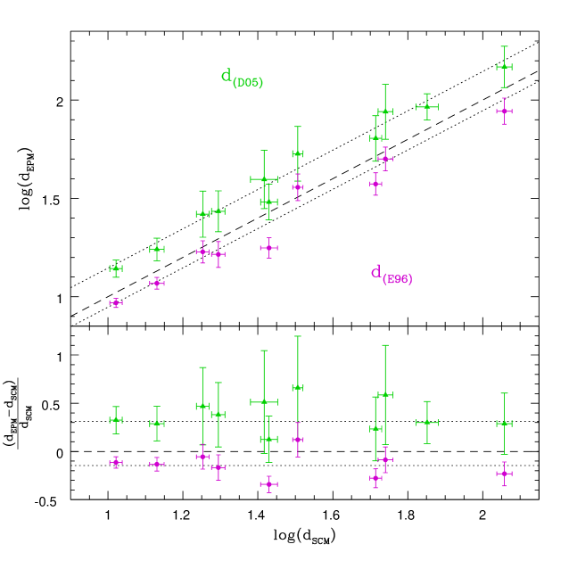
Figure 12: Direct comparison between SCM and EPM distances calculated by Jones et al. (2008). In magenta are shown the EPM distances computed from the atmosphere models of E96, while the green triangles are EPM distances obtained from the D05 models. The bottom panel shows the fractional differences between both techniques against $\log(d_{SCM})$. In both panels the dotted lines trace the systematic shifts of the EPM distances with respect to the SCM distances, $\sim$ 40% and $\sim$ 12% using D05 and E96 atmosphere models, respectively.

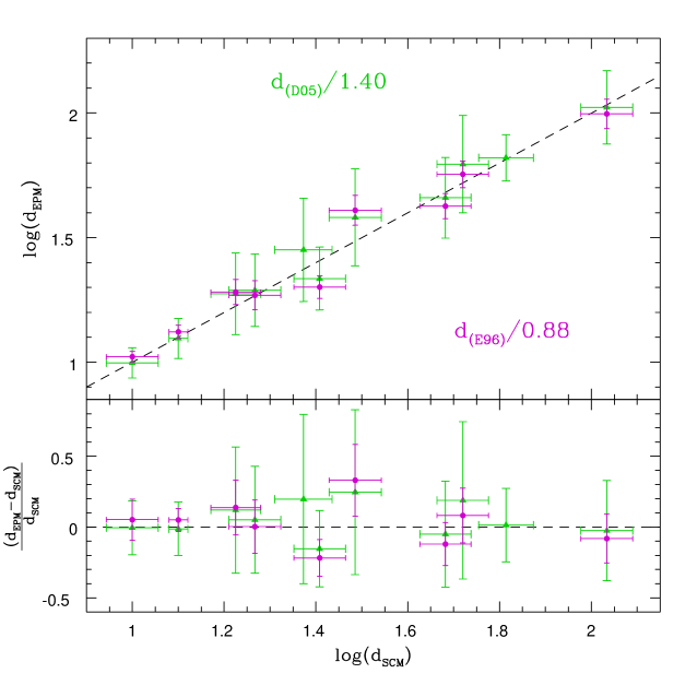
Figure 13: Similar to Figure 12 after bringing the EPM distances to the SCM scale. The removal of the systematic differences leads to random differences between EPM and SCM distances. For the E96 case the discrepancies have a spread of 16%, while for the D05 case the scatter is 13%.

Chapter 4 Discussion

1 Variations of the extinction law

The reddening law that minimizes the dispersion in the $BVI$ Hubble diagrams ($R_{V}=1.4\pm 0.1$) turns out to be very different than the standard Galactic extinction law ($R_{V}=3.1$; Cardelli et al. 1989). To our knowledge this is the first study of the interstellar extinction in external galaxies based on SNe II-P. On the other hand, there have been several studies on this subject using Type Ia SNe. Most recently, Folatelli et al. (2008) solved for $R_{V}$ in a similar manner to our approach, i.e., by minimizing the dispersion in the Hubble diagram and obtained a value of $R_{V}\simeq 1.5$, remarkably consistent with our value. Altavilla et al. (2004) and Reindl et al. (2005) applied a similar procedure by minimizing the dispersion in the $M_{B}-\Delta m_{15}(B)$ relation for SNe Ia and found $R_{B}$ ranging between 3.5 and 3.7, significantly smaller than the standard value of 4.3. An even smaller value of $R_{B}=1.7$ was found by Capaccioli et al. (1990) based on the same kind of analysis for SNe Ia. Further evidence for low $R_{\lambda}$ values were reported by Phillips et al. (1999) and Knop et al. (2003). Studies of individual Type Ia SNe, such as SN 1999cl (Krisciunas et al. 2007), SN 2003cg (Elias-Rosa et al. 2006), SN 2002cv (Elias-Rosa et al. 2008), and SN 2006X (Wang et al. 2008) also yielded low values around $R_{V}\sim 1.5$. Other studies of dust reddening based on diverse methods were performed to nearby galaxies obtaining values for $R_{B}$ ranging between 2.4 and 4.3 (Rifatto 1990; Della Valle & Fanagia 1992; Brosch & Loinger 1991). The ratio of total to selective absorption varies significantly between $R_{V}\simeq 2.6-5.5$ even within our own Galaxy (Clayton & Cardelli 1988). A lower value of $R_{V}$ could be due to dust grains smaller than those in our Galaxy, since for a given value of $A_{V}$ the $E(B-V)$ reddening decreases if the size of the grains grows. On the other hand, Wang (2005) suggests the idea that scattering by dust clouds located in the circumstellar medium of the SN tends to reduce the effective $R_{\lambda}$ in the optical. This effect should be opposite in the ultraviolet, hence it could be further tested with photometry at these wavelenghts.

2 $H_{0}$ comparison with other methods

The HDs constructed from the $V$ – $I$ color at day –30 as the extinction estimator (§ 1) give values of $H_{0}$ between 70–73 km s^-1 Mpc^-1, which turn out to be very similar to those derived from the HDs where we leave $R_{V}$ as a free parameter ($70\pm 8$ km s^-1 Mpc^-1). This shows that if we use $V$ – $I$ color based extinctions, the value of the Hubble constant is not be too sensitive to the adopted $R_{V}$.

Table 1: $H_{0}$ values from the literature

Method	$H_{0}$	Reference
	(km s-1 Mpc-1)
SNe Ia	71$\;\pm\;$2	Freedman et al. (2001)
SNe Ia	71$\;\pm\;$7	Altavilla et al. (2004)
SNe Ia	73$\;\pm\;$4	Riess et al. (2005)
SNe Ia	62$\;\pm\;$1	Sandage et al. (2006)
SNe Ia	72$\;\pm\;$4	Wang et al. (2006)
SNe II-P (EPM)	73$\;\pm\;$6	Schmidt et al. (1994)
SNe II-P (EPM)	52$\;\pm\;$4	Jones et al. (2008)
SNe II-P (EPM)	92$\;\pm\;$7	Jones et al. (2008)
SNe II-P (SCM)	55$\;\pm\;$12	Hamuy & Pinto (2002)
SNe II-P (SCM)	72$\;\pm\;$6	Hamuy (2003)
SNe II-P (EPM)	72$\;\pm\;$9	Freedman et al. (2001)
SNe II-P (SCM)	70$\;\pm\;$8	this study
Tully-Fisher	71$\;\pm\;$3	Freedman et al. (2001)
Tully-Fisher	59$\;\pm\;$2	Sandage et al. (2006)
TRGB	62$\;\pm\;$2	Sandage et al. (2006)
SBF	70$\;\pm\;$5	Freedman et al. (2001)
FP	82$\;\pm\;$6	Freedman et al. (2001)

Table 1 summarizes several modern measurements of the expansion rate of the Universe, $H_{0}$, derived from different methods: SNe Ia, EPM and SCM for SNe II-P, the Tully-Fisher relation, tip of the red giant branch (TRGB) distances, the surface brightness fluctuations (SBF) method, and the “fundamental plane” method for early type galaxies. According to Table 1 the value of the Hubble constant ranges between 52–82 km s^-1 Mpc^-1, and the most accepted value today is 70 km s^-1 Mpc^-1, which is in very good agreement with our SCM value of $70\pm 8$ km s^-1 Mpc^-1.

This study shows that the SCM can deliver accurate distances. The $BVI$ Hubble diagrams yield scatter of 0.3 mag which implies a precision in individual distances $\sim$ 15%. Part of this scatter could be due to the peculiar velocities of the SN host galaxies and the intrinsic precision of SCM could be even lower than this. In fact, when we perform a comparison for SNe in common between SCM and EPM, the distance differences range between 13–16% (after removing the systematic differencce among the SCM and EPM). This comparison is independent of the SN host-galaxy redshifts and implies that the internal precision in any of these two techniques must be lower than 13–16%, since these differences comprise the combined uncertainties of both methods. This is an encouraging result, since it implies that both EPM and SCM can produce high precision relative distances, thus offering a new route to cosmological parameters.

3 Final remarks

We note that the dispersion in the HDs increases with wavelength. This seems contrary to expectations given that 1) the extinction effects decrease with wavelength, and 2) metallicity affects the $B$-band. Perhaps the luminosity is not only a function of velocity but also of metallicity, i.e., $M_{V}=f(\upsilon,\mbox{[Fe/H]})$. If so, the velocity term in eqs. 5–6 might be removing metallicity effects, more efficientlyat shorter wavelengths. This could be tested with [Fe/H] measurements of the Type II-P SNe. We plan to address this issue in the near future. Given the evidence we have, we can only claim a dependence of $L$ with $\upsilon$. The obvious physical explanation is that the internal energy is correlated with the kinetic energy. The implication is that the ratio between the internal energy and kinetic energy is approximately independent of the explosion energy.

Chapter 5 Conclusions

We established a library of 196 SN II optical spectra and developed a code which allows us to correct the observed photometry for Galactic extinction, $K$-terms and host-galaxy extinction. We applied our code to the $BVRI$ photometry of 37 SNe II-P (§ 1). We developed fitting procedures to the light curves, color curves and velocity curves which allow us to precisely determine the transition time between the plateau and the tail phases. The use of this parameter as the time origin permited us to line up the SNe to a common phase. The additional benefit of these fits is the interpolation of magnitudes, colors and velocities over a wide range of epochs. The methodology explained above yields the following conclusions:

1. The comparison between our color-based dereddening technique and the spectroscopic reddenings of Dessart (2008) is satisfactory within the errors of both techniques. This is particularly encouraging since our method uses late-time photometric information, while the other method uses early-time spectroscopic data, i.e. completely independent information.

2. Using our new sample of SNe we recover the luminosity-velocity trend ($LEV$ relation) previously reported by Hamuy & Pinto (2002).

3. We construct $BVI$ HDs using two sets of host-galaxy reddenings. We demonstrated that the ($V$ – $I$)-based extinctions do a much better job than the spectroscopic determinations by Dessart (2008), reaching dispersions of $\sim$ 0.4 mag in the Hubble diagrams. This scatter is somewhat higher than that found previously by Hamuy (2003) of 0.35 mag. A much smaller dispersion of 0.3 mag was achieved when we used $V$ – $I$ colors to estimate reddening and allowed $R_{V}$ to vary. We obtain $R_{V}=1.4\pm 0.1$, much smaller than the Galactic value of 3.1. The low value of $R_{V}$ can be explained by a different nature of the dust grains in host-galaxies along the line of sight to Type II-P SNe.

4. We derive a Hubble constant of $70\pm 8$ km s^-1 Mpc^-1 from $BVI$ photometry, calibrating our HDs with Cepheid distances to SN 1999em and SN 2004dj, which agrees very well with the value obtained by the HST Key Project (Freedman et al. 2001).

5. Finally, we calculate the distance moduli to our SN sample, and make a comparison against EPM distances from Jones et al. (2008). The 11 SNe in common show a systematic difference in distance between EPM and SCM, depending on the atmosphere models employed by EPM. Correcting for these shifts we bring the EPM distances to the SCM distance scale, from which we measure a dispersion of 13–16%. This spread reflects the combined internal precision of EPM and SCM. Therefore the internal precision in any of these two techniques must be $<$ 13–16%.

This analysis reconfirms the usefulness of SNe II-P as cosmological probes, providing strong encouragement to future high-$z$ studies. We found that one can determine relative distances from SNe II-P with a precision of 15% or better. This uncertainty could be further reduced by including more SNe in the Hubble flow. In its current form the SCM requires both photometric and spectroscopic data. Since the latter are expensive to obtain (especially at high-$z$) it would be desirable to look for a photometric observable as a luminosity indicator instead of the expansion velocities.

Chapter 6 The Computation of Synthetic Magnitudes

The implementation of SCM requires the implementation of AKA corrections to the observed SN magnitudes (§ 1). This process involves synthesizing broadband magnitudes from the library of SNe II-P spectra. It is crucial, therefore, to place the synthetic magnitudes on the same photometric system employed in the observations of the SN.

Since the SN magnitudes are measured with photon detectors, a synthetic magnitude is the convolution of the observed photon number distribution, $N_{\lambda}~{}$, with the filter transmission function $S(\lambda)$, i.e.,

$$mag=-2.5~{}log_{10}~{}\int N_{\lambda}~{}S(\lambda)~{}d\lambda~{}+~{}ZP,$$ (1)

where $ZP$ is the zero point for the magnitude scale and $\lambda$ is the wavelength in the observer’s frame.

For an adequate use of equation 1, S($\lambda$) must include the transparency of the Earth’s atmosphere, the filter transmission, and the detector quantum efficiency (QE). For $BVRI$ I adopt the filter functions $B_{90}$, $V_{90}$, $R_{90}$, $I_{90}$ published by Bessell (1990). However, since these curves are meant for use with energy and not photon distributions (see Appendix in  Bessell 1983), I must divide them by $\lambda$ before employing them in equation 1. Also, since these filters do not include the atmospheric telluric lines, I add these features to the $R$ and $I$ filters (in $B$ and $V$ there are no prominent telluric features) using my own atmospheric transmission spectrum. Figure 1 shows the resulting curves.

Figure 1: $BVRI$ filters functions of Bessell (1990) meant for use with energy distributions (dotted curves). With solid lines are shown the curves modified for use with photon distributions, to which I added the telluric lines.

Figure 2: Adopted spectrophotometric calibration for Vega. In the optical ($\lambda$ $\leq$ 10,500 Å) the calibration is from Hayes (1985), and at longer wavelengths I adopted the Kurucz spectrum with parameters $T_{eff}$=9,400 K, log $g$=3.9, [Fe/H]=–0.5, $V_{microturb}$=0.

The $ZP$ in eq. 1 must be determined by forcing the synthetic magnitude of a star to match its observed magnitude. I use the spectrophotometric calibration of Vega published by Hayes (1985) in the range 3300-10405 Å and the $V$ magnitude of 0.03 mag measured by Johnson et al. (1966), from which I solve for the $ZP$ in the $V$-band. In principle, I can use the same procedure for $BRI$, but Vega’s photometry in these bands is not very reliable as it was obtained in the old Johnson standard system. To avoid these problems I employ ten stars with excellent spectrophotometry (Hamuy et al. 1992, 1994) and photometry in the modern Kron-Cousins system (Cousins 1971, 1980, 1984). Before using these standards I remove the telluric lines from the spectra since the filter functions already include these features. With this approach I obtain an average and more reliable zero point for the synthetic magnitude scale with rms uncertainty of $\sim$0.01 mag. With these $ZP$s I find that the synthetic magnitudes of Vega are brighter than the observed magnitudes (Johnson et al. 1966) by 0.016 mag in $B$, 0.025 in $R$, and 0.023 in $I$ (see Table 1), which is not so surprising considering that this comparison requires transforming the Johnson $RI$ magnitudes to the Kron-Cousins system (Taylor 1986). Figure 2 shows the adopted spectrophotometric calibration for Vega.

Table 1: Photometric Zero points and Synthetic Magnitudes for Vega

	$B$	$V$	$R$	$I$
Zero point	35.287	34.855	35.060	34.563
Vega	0.014	0.030	0.042	0.052

Table 1 summarizes the zero points computed with eq. 1, and the corresponding magnitudes for Vega in such system. For the proper use of these $ZP$s it is necessary to express $N_{\lambda}$ in sec^-1 cm^-2 cm^-1 and $\lambda$ in Å. From the ten secondary standards I estimate that the uncertainty in the zero points is $\sim$ 0.01 mag in $BVRI$.

Chapter 7 Finding $\mathcal{F}(\vec{v})$ using the DSM in Multidimensions

Given the 8-parameter function we have to deal with (refer to $\mathcal{F}$ in eq. 5), we had to explore different methods of multidimensional minimization. The Downhill Simplex Method (DSM), due to Nelder & Mead (1965), does not use one-dimensional minimization as a part of their computational strategy. Derivatives are not required, only function evaluations. Its funcionality is based on the simplex, a geometrical figure consisting in $N$ dimensions, of $N+1$ vertices, all their interconecting line segments, and polygonal faces. For example, in 2-dimensional space a simplex is a triangle. The starting guess should not be just a single point, but $N+1$, defining an initial simplex. The DSM now takes a series of steps (shown in Figure 1), most steps just moving the vertice of the simplex where the function is largest through the opposite face of the simplex to a vertice with a lower value of the function. The routine amoeba, called after the unicellular organism, tries to “swallow” the minimum being intended to be descriptive of this kind of behavior. The hungry amoeba is the simplex which is “fed” with minima. The purpose after a few step is the reduction of the $N$-dimensional volume of the simplex as shown in Fig. 1 for the 3D case. Hence the minimum gets enclosed and finally found with an accuracy given by the size of the simplex.

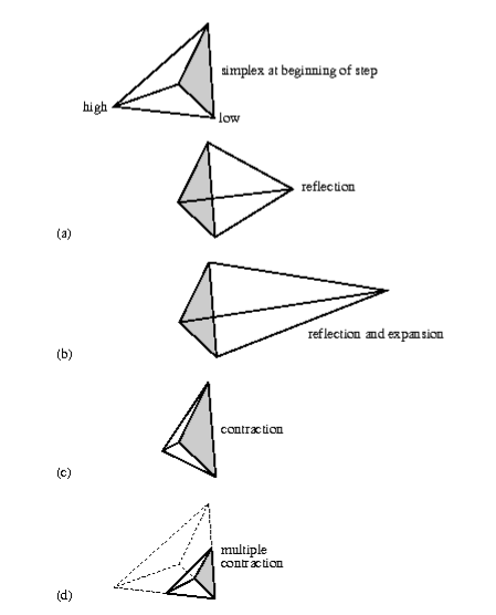
Figure 1: Steps of the amoeba algorithm trying to “swallow” the minimum using the DSM. This example draws the simplex in 3-D (tetrahedron). The possible outcomes, that move away from the highest point, are (a) the vertice is reflected through its opposite face, (b) a reflection plus a 1-D expansion, and (c) a 1-D contraction. A more unusual step performs (d) a contraction along all dimensions towards the lowest vertice.

The input parameters for the Fortran version of this routine are the following

amoeba(isimplex[mp,np],y[mp],mp,np,ndim,ftol,funk,iter)

where

isimplex[mp,np] : the matrix containing the coordinates of the initial simplex, np+1 vertices defined by a np-dimensional vector

y[mp] : vector composed by the value function evaluated in each of the np+1 initial vertices (rows) of isimplex

mp = np + 1

np = ndim

ndim : number of dimensions or variables of the function (parameters to be fitted)

ftol : the fractional convergence tolerance to be achieved in the value of the function

funk : function of the form funk(x) where x[mp] is a np+1-dimensional vector

iter : total number of function evaluations after the convergence

The output consists of the isimplex matrix and the y vector overwritten by np+1 new points all within a tolerance ftol of the minimum function value, whereas the number of function evaluations is saved in iter. Thus, the result is a new and smaller simplex containing the minimum. This procedure guarantees a succesful search of at least a local minimum value of the function.

In our specific case we want to minimize $\chi^{2}(\vec{v})$ as a function of the parameter vector $\vec{v}$, which is written as

$$\chi^{2}(\vec{v})=\sum_{i=1}^{nobs}\left(\frac{mag[i]-\mathcal{F}(\vec{v};t[i])}{\sigma_{mag}[i]}\right)^{2}$$ (1)

where $\mathcal{F}$ is the function defined in eq. 8 whose role is to model the SNe II-P light curves. ($mag[i]\,\pm\,\sigma_{mag}[i]$) is the observed magnitude of the SN with its associated uncertainty for a given Julian date $t[i]$, all together completing a total of $nobs$ measurements that, basically, draw the observed SN light curve.

Although simple and user-friendly, the DSM finds problems working on an 8-dimensional space but not as most algorithm would do. In most cases the initial simplex has to be accurately defined according to the desired results. In order to make a semi-automatic search for the initial simplex, we introduce new parameters in the minimization routine. From the photometric observations we extract the date of the first data point $t_{i}$, and using a simple algorithm we calculate the approximate end of the plateau $t_{end}$ (refer to § 1). By means of these calculations we constrain the $\mathcal{F}$-parameters having temporal components. In order to contract the magnitude component of the $\mathcal{F}$-parameters we extract from the photometry the brightest and the dimmest magnitude, $m_{bri}$ and $m_{dim}$ respectively. For example, below is shown the initial simplex we feed into amoeba to fit the V light curve of SN 1999em,

$$\mbox{\tt isimplex}={\small\bordermatrix{&a_{0}&t_{PT}&w_{0}&p_{0}&m_{0}&P&Q&R\cr&4&t_{end}-5&4.5&0.08&m_{bri}&-1.2&60&t_{i}+9\cr&1.6&t_{end}+25&45&0.08&m_{bri}&-1.2&60&t_{end}-10\cr&1.6&t_{end}-5&8&0.08&m_{bri}&-1.2&60&t_{end}-10\cr&1.6&t_{end}-5&4.5&0.012&m_{bri}&-1.2&60&t_{end}-10\cr&1.6&t_{end}-5&4.5&0.08&25&-1.2&60&t_{end}-10\cr&1.6&t_{end}-5&4.5&0.08&m_{bri}&1.7&60&t_{end}-10\cr&1.6&t_{end}-5&4.5&0.08&m_{bri}&-1.2&21&t_{end}-10\cr&1.6&t_{end}-5&4.5&0.08&m_{bri}&-1.2&60&t_{end}-10\cr&4&t_{end}+25&8&0.012&25&1.7&60&t_{i}+9\cr}},$$ (2)

where the rows are the 9 initial vertices of the simplex in the 8-parameter coordinate system. This is one structure of the many one can choose to build the isimplex that gives us the best convergence. Each filter requires slightly different parameter ranges. By averaging the vertices of the final converging simplex, we obtain a unique parameter vector with its corresponding uncertainty vector calculated from the dispersions of the 9 vertices around the mean. The resulting fits for SN 1999em are shown in the upper-right panel of Fig. 4 and the corresponding parameters are summarized in Table 1.

Table 1: $\mathcal{F}$-parameters for the V light curve of SN 1999em

$a_{0}$	1.978$\,\pm\,$	0.015	mag
$t_{PT}$	JD 2451590.1$\,\pm\,$	1.1
$w_{0}$	4.52$\,\pm\,$	0.85	day
$p_{0}$	9.0$\,\pm\,$	0.4	10${}^{-3}\,$mag/day
$m_{0}$	16.297$\,\pm\,$	0.014	mag
$P$	–0.403$\,\pm\,$	0.019	mag
$Q$	JD 2451475.3$\,\pm\,$	3.7
$R$	64.6$\,\pm\,$	5.7	day

References

- Altavilla et al. (2004) Altavilla, G., et al. 2004, MNRAS, 349, 1344
- Anderson & James (2008) Anderson, J. P., & James, P. A. 2008, private communication
- Arnett (1996) Arnett, D. 1996, Supernovae and Nucleosynthesis, (New Jersey: Princeton Univ. Press)
- Astier et al. (2006) Astier, P., et al. 2006, A&A, 447, 31
- Baade & Zwicky (1934) Baade, W., & Zwicky, F. 1934, Physical Review , 46, 76
- Barbon et al. (1979) Barbon, R., Ciatti, F., & Rosino, L. 1979, A&A, 72, 287
- Barbon et al. (1990) Barbon, R., Benetti, S., Rosino, L., Cappellaro, E., & Turatto, M. 1990, A&A, 237, 79
- Bennett et al. (2003) Bennett, C. L., et al. 2003, ApJS, 148, 1
- Bersten et al. (2008) Bersten, M., Benvenuto, O., & Hamuy, M. 2008, in preparation
- Bessell (1983) Bessell, M. S. 1983, PASP, 95, 480
- Bessell (1990) Bessell, M. S. 1990, PASP, 102, 1181
- Blake & Glazebrook (2003) Blake, C., & Glazebrook, K. 2003, ApJ, 594, 665
- Brosch & Loinger (1991) Brosch, N., & Loinger, F. 1991, A&A, 249, 327
- Burrows (2000) Burrows, A. 2000, Nature, 403, 727
- Capaccioli et al. (1990) Capaccioli, M., Cappellaro, E., della Valle, M., D’Onofrio, M., Rosino, L., & Turatto, M. 1990, ApJ, 350, 110
- Capaccioli et al. (2003) Capaccioli, M., Cappellaro, E., Mancini, D., & Sedmak, G. 2003, Memorie della Societa Astronomica Italiana Supplement, 3, 286
- Cardelli et al. (1989) Cardelli, J. A., Clayton, G. C., & Mathis, J. S. 1989, ApJ, 345, 245
- Castander (2007) Castander, F. J. 2007, Cosmic Frontiers, 379, 285
- Clayton & Cardelli (1988) Clayton, G. C., & Cardelli, J. A. 1988, AJ, 96, 695
- Cleveland et al. (1992) Cleveland, W. S., Grosse, E., & Shyu W. M. 1992, Local Regression models. Chapter 8 of Statistical Models in S, eds J. M. Chambers and T. J. Hastie, Wadsworth & Brooks/Cole
- Cousins (1971) Cousins, A. W. J. 1971, Royal Observatory Annals, 7, C
- Cousins (1980) Cousins, A. W. J. 1980, South African Astronomical Observatory Circular, 1, 234
- Cousins (1984) Cousins, A. W. J. 1984, South African Astronomical Observatory Circular, 8, 69
- Della Valle & Fanagia (1992) Della Valle, M., & Fanagia, N. 1992, AJ, 104, 696
- Dessart & Hillier (2005) Dessart, L., & Hillier, D. J. 2005, A&A, 439, 671
- Dessart (2008) Dessart, L. 2008, private communication
- Eastman et al. (1996) Eastman, R. G., Schmidt, B. P. & Kirshner, R. 1996, ApJ, 466, 911
- Elias-Rosa et al. (2006) Elias-Rosa, N., et al. 2006, MNRAS, 369, 1880
- Elias-Rosa et al. (2008) Elias-Rosa, N., et al. 2008, MNRAS, 384, 107
- Emerson et al. (2004) Emerson, J. P., Sutherland, W. J., McPherson, A. M., Craig, S. C., Dalton, G. B., & Ward, A. K. 2004, The Messenger, 117, 27
- Filippenko (1997) Filippenko, A. V. 1997, ARA&A, 35, 309
- Fixsen et al. (1996) Fixsen, D. J., Cheng, E. S., Gales, J. M., Mather, J. C., Shafer, R. A., & Wright, E. L. 1996, ApJ, 473, 576
- Folatelli et al. (2008) Folatelli, G., et al. 2008, in preparation
- Freedman et al. (2001) Freedman, W. L., et al. 2001, ApJ, 553, 47
- Granlund et al. (2006) Granlund, A., Conroy, P. G., Keller, S. C., Oates, A. P., Schmidt, B., Waterson, M. F., Kowald, E., & Dawson, M. I. 2006, Proc. SPIE, 6269, 69
- Hamuy et al. (1990) Hamuy, M., Suntzeff, N. B., Bravo, J., & Phillips, M. M. 1990, PASP, 102, 888
- Hamuy et al. (1992) Hamuy, M., Walker, A. R., Suntzeff, N. B., Gigoux, P., Heathcote, S. R., & Phillips, M. M. 1992, PASP, 104, 533
- Hamuy et al. (1992, 1994) Hamuy, M., Suntzeff, N. B., Heathcote, S. R., Walker, A. R., Gigoux, P., & Phillips, M. M. 1994, PASP, 106, 566
- Hamuy et al. (1996) Hamuy, M., Phillips, M. M., Suntzeff, N. B., Schommer, R. A., Maza, J., & Aviles, R. 1996, AJ, 112, 2391
- Hamuy et al. (1996) Hamuy, M., Phillips, M. M., Suntzeff, N. B., Schommer, R. A., Maza, J., & Aviles, R. 1996, AJ, 112, 2398
- Hamuy et al. (2001) Hamuy, M., et al. 2001, ApJ, 558, 615
- Hamuy (2001) Hamuy, M. 2001, Ph.D. thesis, Univ. Arizona
- Hamuy & Pinto (2002) Hamuy, M., & Pinto, P. A. 2002, ApJ, 566, L63
- Hamuy (2003) Hamuy, M. 2003, ArXiv Astrophysics e-prints, arXiv:astro-ph/0309122
- Hamuy et al. (2008) Hamuy, M., et al. 2008, in preparation
- Hayes (1985) Hayes, D. S. 1985, in Calibration of Fundamental Stellar Quantities, ed. D. S. Hayes, L. E. Pasinetti, & A. G. Philip (Dordrecht: Reidel), 225
- Hendry et al. (2005) Hendry, M. A., et al. 2005, MNRAS, 359, 906
- Hillebrandt & Niemeyer (2000) Hillebrandt, W., & Niemeyer, J. C. 2000, ARA&A, 38, 191
- Hobbs (1974) Hobbs, L. M., 1974, ApJ, 191, 381
- Hodapp et al. (2004) Hodapp, K. W., et al. 2004, Astronomische Nachrichten, 325, 636
- Jha et al. (2007) Jha, S., Riess, A. G., & Kirshner, R. P. 2007, ApJ, 659, 122
- Johnson et al. (1966) Johnson, H. L., Iriarte, B., Mitchell, R. I., & Wisniewski, W. Z. 1966, Commun. Lunar Plan. Lab., 4, 99
- Jones et al. (2008) Jones, M., et al. 2008, in preparation
- Knop et al. (2003) Knop, R. A., et al. 2003, ApJ, 598, 102
- Kirshner & Kwan (1974) Kirshner, R. P., & Kwan, J. 1974, ApJ, 193, 27
- Krisciunas et al. (2007) Krisciunas, K., et al. 2007, AJ, 133, 58
- Landolt (1992) Landolt, A. U. 1992, AJ, 104, 340
- Leonard et al. (2002) Leonard, D. C., et al. 2002, PASP, 114, 35
- Leonard et al. (2002) Leonard, D. C., et al. 2002, AJ, 124, 2490
- Li et al. (2001) Li, W., Filippenko, A. V., Treffers, R. R., Riess, A. G., Hu, J., & Qiu, Y. 2001, ApJ, 546, 734
- Munari & Zwitter (1997) Munari, U., & Zwitter, T. 1997, AJ, 318, 269
- Nadyozhin (2003) Nadyozhin, D. K. 2003, MNRAS, 346, 97
- Minkowski (1941) Minkowski, R. 1941, PASP, 53, 224
- Nelder & Mead (1965) Nelder, J. A., & Mead, R. 1965, Computer Journal, vol. 7, 308, 313
- Nugent et al. (2006) Nugent, P., et al. 2006, ApJ, 645, 841
- Pastorello et al. (2006) Pastorello, A., et al. 2006, MNRAS, 370, 1752
- Perlmutter et al. (1999) Perlmutter, S., et al. 1999, ApJ, 517, 565
- Phillips (1993) Phillips, M. M. 1993, ApJ, 413, L105
- Phillips et al. (1999) Phillips, M. M., Lira, P., Suntzeff, N. B., Schommer, R. A., Hamuy, M., & Maza, J. 1999, AJ, 118, 1766
- Press et al. (1992) Press, W. H., Teukolsky, S. A., Vetterling, W. T., & Flannery, B. P. 1992, Numerical Recipes in Fortran, (2nd ed; Cambridge: Cambridge University Press), 686
- Prieto et al. (2006) Prieto, J. L., Rest, A., & Suntzeff, N. B. 2006, ApJ, 647, 501
- Reindl et al. (2005) Reindl, B., Tammann, G. A., Sandage, A., & Saha, A. 2005, ApJ, 624, 532
- Riess et al. (1998) Riess, A. G., et al. 1998, AJ, 116, 1009
- Riess et al. (2005) Riess, A. G., et al. 2005, ApJ, 627, 579
- Rifatto (1990) Rifatto, A. 1990, in Bussoletti E., Vittone A. A., eds, Dusty Objects in The Universe. Kluwer, Dordrecht, p. 277
- Sahu et al. (2006) Sahu, D. K., Anupama, G. C., Srividya, S., & Muneer, S. 2006, MNRAS, 372, 1315
- Sakai et al. (2004) Sakai, S., Ferrarese, L., Kennicutt, R. C., Jr., & Saha, A. 2004, ApJ, 608, 42
- Sandage et al. (2006) Sandage, A., Tammann, G. A., Saha, A., Reindl, B., Macchetto, F. D., & Panagia, N. 2006, ApJ, 653, 843
- Schneider et al. (1983) Schneider, D. P., Gunn, J. E., & Hoessel, J. G. 1983, ApJ, 264, 337
- Svoboda et al. (1987) Svoboda, R., et al. 1987, IAU Circ., 4340, 1
- Seo & Eisenstein (2003) Seo, H.-J., & Eisenstein, D. J. 2003, ApJ, 598, 720
- Schlegel et al. (1998) Schlegel, D. J., Finkbeiner, D. P., & Davis, M. 1998, ApJ, 500, 525
- Schmidt et al. (1994) Schmidt, B. P., Kirshner, R. P., Eastman, R. G., Phillips, M. M., Suntzeff, N. B., Hamuy, M., Maza, J., & Aviles, R. 1994, ApJ, 432, 42
- Spergel et al. (2007) Spergel, D. N., et al. 2007, ApJS, 170, 377
- Taylor (1986) Taylor, B. J. 1986, ApJS, 60, 577
- Tonry & Schneider (1988) Tonry, J., & Schneider, D. P. 1988, AJ, 96, 807
- Tsvetkov et al. (2006) Tsvetkov, D. Y., Volnova, A. A., Shulga, A. P., Korotkiy, S. A., Elmhamdi, A., Danziger, I. J., & Ereshko, M. V. 2006, A&A, 460, 769
- Tyson et al. (2003) Tyson, J. A., Wittman, D. M., Hennawi, J. F., & Spergel, D. N. 2003, Nuclear Physics B Proceedings Supplements, 124, 21
- Utrobin (2007) Utrobin, V. P. 2007, A&A, 461, 233
- Van Dyk et al. (2003) Van Dyk, S. D., Li, W., & Filippenko, A. V. 2003, PASP, 115, 1289
- Vinkó et al. (2006) Vinkó, J., et al. 2006, MNRAS, 369, 1780
- Wang (2005) Wang, L. 2005, ApJ, 635, L33
- Wang et al. (2006) Wang, X., Wang, L., Pain, R., Zhou, X., & Li, Z. 2006, ApJ, 645, 488
- Wang et al. (2008) Wang, X., et al. 2008, ApJ, 675, 626
- Weaver & Woosley (1980) Weaver, T. A., & Woosley, S. E. 1980, Ninth Texas Symposium on Relativistic Astrophysics, pp. 335–357, 335
- Wood-Vasey et al. (2007) Wood-Vasey, W. M., et al. 2007, ApJ, 666, 694