Determination of atomic scattering lengths from measurements of molecular binding energies near Feshbach resonances

Abstract

We present an analytic model to calculate the atomic scattering length near a Feshbach resonance from data on the molecular binding energy. Our approach considers finite-range square-well potentials and can be applied near broad, narrow, or even overlapping Feshbach resonances. We test our model on Cs₂ Feshbach molecules. We measure the binding energy using magnetic-field modulation spectroscopy in a range where one broad and two narrow Feshbach resonances overlap. From the data we accurately determine the Cs atomic scattering length and the positions and widths of two particular resonances.

I Introduction

In experiments on ultracold quantum gases, control of the atomic scattering length near Feshbach resonances has become a powerful tool to explore different interaction regimes FBreview . Prominent examples include the implosion and explosion of Bose-Einstein condensates wieman2001 , the creation of ultracold molecules FM ; ferlbook , strongly interacting Fermi gases xoverexp ; giorgrevi , and the observation of three-body Efimov states Kraemer2006 . Moreover, Feshbach resonances have been proposed as a very sensitive probe to the variation of fundamental constants fundamental .

For all such experiments precise knowledge of the atomic scattering length $a$ is desirable. Usually a multi-channel molecular potential model is employed to calculate the scattering length. This approach requires experimental input, as usually provided by photoassociative or Feshbach spectroscopic data Tiesinga1996 ; Abraham1997 ; Marte2002 . It captures the global scattering behavior of the system and has a predictive power on Feshbach resonance positions with an uncertainty of typically a few hundred milligauss. In many experimental situations, however, precise knowledge of $a$ is needed in the vicinity of specific Feshbach resonances at a level not reachable with this global approach.

We here consider the situation in which the scattering length $a$ near a specific resonance is calculated using molecular binding energy data. Nowadays powerful experimental methods are available to measure the binding energy of Feshbach molecules with very high accuracy, such as radio-frequency and microwave spectroscopy regal2003 ; boundbound ; Claussen2003 ; Thompson2005 ; Papp2006 . For the relation between the binding energy $E_{\rm b}$ and $a$ a simple analytic form can be given in the universal limit of very large positive values of $a$. It is given by $E_{\rm b}=\hbar^{2}/(2m_{r}a^{2})$, with $m_{r}$ being the reduced mass. In general, the relation between molecular binding energy and scattering length is more complex, depending also on short-range parameters of the molecular potentials. In principle one may also use a multi-channel calculation to precisely derive $a$ from measurements of $E_{\rm b}$. When the specific scattering properties are needed near a particular Feshbach resonance, a much more simple model can be applied.

In this Article, we describe a versatile analytic model to directly convert molecular binding energy data into atomic scattering lengths near Feshbach resonances. Our approach considers square-well model potentials and can be applied to any broad or narrow Feshbach resonance, or even to the case of overlapping resonances. We demonstrate our model on Cs₂ Feshbach molecules. Cesium is an excellent candidate to test scattering models because of its rich interaction properties Chin2004 ; Mark2007 . From fitting the binding energy data, we show that the magnetic-field dependent scattering length can be determined with high precision. We compare our results with the full multi-channel numerical calculation of Ref. Chin2004 .

II Feshbach resonance model

We employ a two-channel square well potential $\hat{V}(R)$ to describe interacting atoms and weakly-bound molecules near a Feshbach resonance. The well size is chosen to account for the long range behavior of the molecular potential, which is dominated by the van der Waals (vdW) interaction $V(R)=-C_{6}/R^{6}$, where $C_{6}$ is the vdW coefficient and $R$ is the atomic separation. The associated vdW length scale and vdW energy scales are $R_{\mathrm{vdW}}=\frac{1}{2}(2m_{r}C_{6}/\hbar^{2})^{1/4}$ and $E_{\mathrm{vdW}}=\hbar^{2}/2m_{r}R_{\mathrm{vdW}}^{2}$.

To fully capture the threshold behavior of atomic scattering with vdW interaction, the well size is chosen to be the mean scattering length $\bar{a}=4\pi\Gamma(1/4)^{-2}R_{\mathrm{vdW}}$ Gribakin1993 , where $\Gamma(x)$ is the gamma function. This choice yields the same binding energy of weakly-bound molecules in the vdW potential, namely, $E_{b}=\hbar^{2}/2m_{r}(a-\bar{a})^{2}$ for $E_{b}\ll E_{\mathrm{vdW}}$ Gribakin1993 .

In our model, scattering atoms are initially prepared in one spin configuration, called the “entrance channel” $|e\rangle$. A second “closed channel” $|c\rangle$ supports a molecular bound state, see Fig. 1. The quantum state of an atomic pair with energy $E$ is described as $|\psi\rangle=\psi_{c}(R)|c\rangle+\psi_{e}(R)|e\rangle$, which satisfies Schrödinger’s equation:

$$\left(-\frac{\hbar^{2}}{2m_{r}}\nabla^{2}+\hat{V}\right)|\psi\rangle=E|\psi\rangle$$ (1)

where, using a matrix representation, we write

$$\hat{V} = \left[\begin{array}[]{cc}-V_{c}&\hbar\Omega\\ \hbar\Omega&-V_{e}\end{array}\right]\mbox{ for $R<\bar{a}$,}$$ (4)

$$= \left[\begin{array}[]{cc}\infty&0\\ 0&0\end{array}\right]\,\,\,\mbox{ for $R>\bar{a}.$}$$ (7)

Here for $R<\bar{a}$, we assume the attractive potential can support multiple molecular states, that is, $V_{e},V_{c}\gg E_{\mathrm{vdW}}$, and $\hbar\Omega$ induces Feshbach coupling between the channels. For $R>\bar{a}$, entrance and closed channel thresholds are set to be $E=0$ and $E=\infty$, respectively. See Fig. 1.

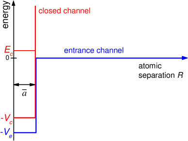
Figure 1: (color online) Two-channel square well model of Feshbach resonances. Scattering states are initially prepared in the entrance channel $|e\rangle$; the closed channel $|c\rangle$ supports a bare bound state at energy $E_{c}$. Feshbach coupling is modeled by the mixing of the two channels, which is resonantly enhanced when the bound state is near the scattering state. The interaction range is set to be the mean-scattering length of the atomic van der Waals potential, see text.

II.1 Scattering state above threshold and scattering length

For $E=\hbar^{2}k^{2}/2m_{r}>0$, the solution of Eq. (1) corresponds to an eigenstate lying above the entrance-channel threshold and is given by

$$|\psi\rangle \propto \frac{\sin(q_{+}R)}{R}|+\rangle+\frac{A\sin(q_{-}R)}{R}|-\rangle\,\,\,\mbox{for $R<\bar{a}$}$$ (8)

$$\propto \frac{\sin(kR+\eta)}{R}|e\rangle\,\,\,\mbox{ for $R>\bar{a}$},$$ (9)

where $A$ is a constant, $\hbar^{2}q_{\pm}^{2}/2m_{r}=E+\frac{1}{2}(V_{e}+V_{c})\pm\frac{1}{2}(V_{e}-V_{c})\sec 2\theta$, $\tan 2\theta=2\hbar\Omega/(V_{e}-V_{c})$, $|+\rangle=\cos\theta|e\rangle+\sin\theta|c\rangle$ and $|-\rangle=-\sin\theta|e\rangle+\cos\theta|c\rangle$. The scattering phase shift $\eta$ can be derived from the continuity condition of the wavefunction at $R=\bar{a}$, which gives

$$\frac{k}{\tan{(k\bar{a}+\eta)}}=\frac{q_{+}\cos^{2}\theta}{\tan{(q_{+}\bar{a})}}+\frac{q_{-}\sin^{2}\theta}{\tan{(q_{-}\bar{a})}}.$$ (10)

Potential depths $V_{c}$ and $V_{e}$ can be chosen such that in the weak coupling limit $\theta\rightarrow 0$, the scattering phase shift approaches the off-resonant value $\eta_{\mathrm{bg}}$ and the closed channel bound state is at $E_{c}$. These two conditions, given by

$$\frac{q_{+}}{\tan{(q_{+}\bar{a})}}=\frac{k}{\tan{(k\bar{a}+\eta_{\mathrm{bg}})}}$$ (11)

$$\sin\left(\hbar^{-1}\sqrt{2m_{r}(E_{c}+V_{c})}\bar{a}\right)=0,$$ (12)

allow us to eliminate $q_{+}$ and $q_{-}$ in Eq. (10). Assuming further that only one bare bound state is near the continuum $|E_{c}|\ll\sqrt{V_{c}E_{\rm vdW}}$, and the Feshbach coupling is weak $|\theta|\approx\hbar\Omega/|V_{e}-V_{c}|\ll 1$, we get

$$\cot(k\bar{a}+\eta)=\cot(k\bar{a}+\eta_{\mathrm{bg}})-\frac{\Gamma/2}{k\bar{a}E_{c}},$$ (13)

where we have introduced the Feshbach coupling strength $\Gamma/2=2\theta^{2}V_{c}$.

Scattering lengths can be derived from the threshold relation $a=-\lim_{k\rightarrow 0}(k\cot\eta)^{-1}$. From Eq. (13), we get

$$\frac{1}{a-\bar{a}}=\frac{1}{a_{\mathrm{bg}}-\bar{a}}+\frac{\Gamma/2}{\bar{a}E_{c}},$$ (14)

where $a_{\mathrm{bg}}=-\lim_{k\rightarrow 0}(k\cot\eta_{\mathrm{bg}})^{-1}$ is the background scattering length.

Magnetic tunability of Feshbach resonances can be modeled by a linear Zeeman shift of the bare bound state as $E_{c}=\delta\mu(B-B_{c})$, where $B$ is the magnetic field, $\delta\mu$ is the relative magnetic moment of the two channels, and $B_{c}$ is magnetic field that tunes the bare state to the entrance channel threshold. This magnetic field dependence allows us to rewrite the scattering length in the standard resonance form $a=a_{\mathrm{bg}}[1-\Delta/(B-B_{0})]$. Here the resonance width $\Delta$ and position $B_{0}$ are given by

$$\Delta = \delta\mu^{-1}\alpha\frac{\Gamma}{2},$$ (15)

$$B_{0} = B_{c}-\beta\Delta,$$ (16)

where $\alpha=(a_{\mathrm{bg}}-\bar{a})^{2}/a_{\mathrm{bg}}\bar{a}$ and $\beta=a_{\mathrm{bg}}/(a_{\mathrm{bg}}-\bar{a})$ are dimensionless parameters.

II.2 Bound molecular state below threshold

We assume that a bound eigenstate $|\psi_{m}\rangle$ is located near and below the continuum with binding energy $E_{b}=\hbar^{2}k_{m}^{2}/2m_{r}$. Solving Eq. (1), we obtain the wave function as

$$|\psi_{m}(R>\bar{a})\rangle \propto \frac{\exp(-k_{m}R)}{R}\,|e\rangle,$$

$$|\psi_{m}(R<\bar{a})\rangle \propto \frac{\sin(\bar{q}_{+}R)}{R}|+\rangle+\frac{A_{m}\sin(\bar{q}_{-}R)}{R}|-\rangle,$$

where $A_{m}$ is a constant and $\bar{q}_{\pm}=(q_{\pm}^{2}-k^{2}-k_{m}^{2})^{1/2}$.

The binding energy $E_{b}$ can be determined from the boundary conditions at $R=\bar{a}$. Following the same calculation as that leading to Eq. (14), we find that for large background scattering length $|a_{\mathrm{bg}}|\gg\bar{a}$, the wave-number $k_{m}$ determining the binding energy $E_{b}=\hbar^{2}k_{m}^{2}/2m_{r}$ satisfies

$$k_{m}=\frac{1}{a_{\mathrm{bg}}-\bar{a}}+\frac{\Gamma/2}{\bar{a}(E_{b}+E_{c})}.$$ (17)

In the limit when the Feshbach coupling approaches zero $\Gamma\rightarrow 0$, the eigenenergies reduce to $E_{b}=-E_{c}$ and $E_{b}=\hbar^{2}/2m_{r}(a_{\mathrm{bg}}-\bar{a})^{2}$ (for $a_{\mathrm{bg}}>\bar{a}$), which correspond to the uncoupled bare states in the closed and entrance channels, respectively.

One can now convert the binding energy into the scattering length with the following strategy. First, the binding energy data are fitted with Eq. (17). The fitting parameters are $\delta\mu$, $\Gamma$, $a_{\rm bg}$, and $B_{c}$. Usually the mean scattering length $\bar{a}$ is fixed because of sufficient knowledge of $C_{6}$. In some cases, also $a_{\mathrm{bg}}$ or $\delta\mu$ are known so that they can be kept fixed during the fit procedure. Second, one determines the width $\Delta$ and the location of the Feshbach resonance $B_{0}$ from the fitting parameters using Eq. (15) and (16).

II.3 Multiple overlapping Feshbach resonances

The above discussed model can be generalized to the case of multiple, overlapping Feshbach resonances, which commonly occurs in cold collisions of alkali atoms and chromium atoms.

Let us assume that $N$ weakly-bound states are supported by $N$ independent closed channels. If the mixing between the closed channels and the entrance channel are weak and $|a_{\mathrm{bg}}|\gg\bar{a}$, we can extend Eq. (1) to model the scattering length and molecular energy. The results are

$$\frac{1}{a-\bar{a}} = \frac{1}{a_{\mathrm{bg}}-\bar{a}}+\frac{1}{\bar{a}}\sum^{N}_{i}\frac{\Gamma_{i}/2}{E_{i}}$$ (18)

$$k_{m} = \frac{1}{a_{\mathrm{bg}}-\bar{a}}+\frac{1}{\bar{a}}\sum^{N}_{i}\frac{\Gamma_{i}/2}{E_{b}+E_{i}},$$ (19)

where $E_{i}$ is the energy of the $i$th bare bound state and $\Gamma_{i}$ is its Feshbach coupling strength to the entrance channel. The results presented here bear similarity to those from the classic Fano theory on the coupling of discrete states to a continuum fano1961 .

Assuming the bare states can be linearly tuned magnetically, namely, $E_{i}=\delta\mu_{i}(B-B_{c,i})$, where $\delta\mu_{i}$ is the relative magnetic moment and $B_{c,i}$ is the crossing field value of the $i$-th bare bound state, we can express the scattering length as $a/a_{\mathrm{bg}}=1-P(B)/Q(B)$, where $P(x)$ and $Q(x)$ are polynomials of $(N-1)$- and $N$-th order, respectively. If we further assume all $B_{c,i}$’s are distinct and all $\mu_{i}$’s have the same sign, the scattering length expression can be factorized as:

$$\frac{a}{a_{\mathrm{bg}}}=\prod^{N}_{i=1}\frac{B-B^{*}_{i}}{B-B_{0,i}}.$$ (20)

Here we define $B_{0,i}$ as the $i$-th lowest pole of $a/a_{\mathrm{bg}}$, and $B^{*}_{i}$ the $i$-th lowest zero. This form is more convenient for experimental research since zeros and poles of the scattering length can be identified experimentally. Accordingly, the width of the $i$-th Feshbach resonance can be defined as $\Delta_{i}=B^{*}_{i}-B_{0,i}$.

III Binding energy measurements and determination of the scattering length

III.1 Measurements of the binding energy

We measure the binding energies of ultracold Cs₂ Feshbach molecules in a magnetic field range where a weakly bound $s$-wave molecular state overlaps with a $d$-wave and a $g$-wave state Mark2007 . The latter two states are connected to the $d$-wave and $g$-wave Feshbach resonances located at about $48$ G and $53.5$ G, respectively Chin2004 . The molecular spectroscopy is performed by using a weak oscillating magnetic field. This technique, previously applied to a ⁸⁵Rb atomic sample Thompson2005 and to a ⁸⁵Rb-⁸⁷Rb mixture Papp2006 , has the advantage to determine binding energies of weakly bound molecules to within a few percent. The oscillating magnetic field stimulates a transition between an atom pair and a molecule for a modulation frequency resonant to $E_{b}/h$ Thompson2005 ; Hanna2007 , where $h$ is the Planck constant.

Our molecular spectroscopy is performed using ultracold Cs atoms in an optical trap. A detailed description of our experimental procedure can be found in Ref. Rychtarik2004 . After several pre-cooling stages, the atoms are fully polarized in their absolute ground state $|F\!=\!3,m_{F}\!=\!3\rangle$. We evaporatively cool the atoms in the optical trap at a magnetic field of 27 G surfacetrap , where the two-body scattering length is large enough ($a\approx$ 450$a_{0}$, with $a_{0}$ the Bohr radius) to provide fast thermalization. During the evaporation sequence, an extra magnetic field gradient is applied to levitate the atoms against the gravity Chin2005 ; Weber2003 . We typically obtain a nearly-degenerate sample of 8000 Cs atoms at $T=100$ nK. Typical values for the density and phase space density are $1.2\times 10^{12}$ cm^-3 and 0.2, respectively.

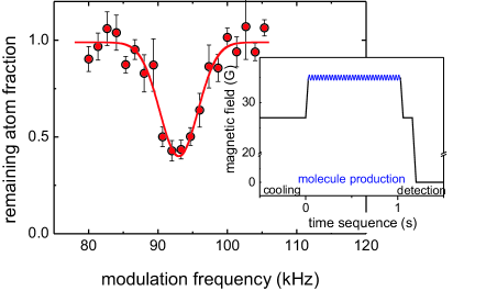
Figure 2: (color online). Example of a loss resonance at 48.2 G. The losses are due to the coupling between atom pairs and $d$-wave molecules. The solid line is a gaussian fit to the data. We find the resonant frequency to be $\nu=93.0(3)$ kHz and the width 5.5(6) kHz. The inset shows the typical magnetic field sequence used to associate Cs₂ molecules with an oscillating magnetic field.

We measure the molecular binding energy by magnetic field modulation Thompson2005 ; Hanna2007 . The inset of Fig. 2 shows the magnetic-field sequence. After ramping the magnetic field within 3 ms to a desired value in the range of interest, we add for typically 1 s a small sinusoidal magnetic field $B(t)=A\sin(2\pi\nu t)$, where the modulation amplitude $A$ typically ranges from 100 to 600 mG. We then ramp back the magnetic field to initial value and wait 100 ms, during which the associated molecules decay by inelastic collisions with the atoms. The magnetic field is then rapidly turned off to image the atoms with standard absorption imaging technique. If the modulation frequency $\nu$ is close to the binding energy value, $E_{\rm b}\simeq h\nu$, the oscillating magnetic field couples atom pairs to molecules Hanna2007 . The atoms are converted into molecules, and the resulting association is detected as resonant loss in the atom number. A typical loss signal is shown in Fig. 2. The resonant frequency is determined to within a few percent by fitting the data with a Gaussian profile BR .

We determine the resonant loss frequency for different values of the magnetic field. Figure 3 shows the measured molecular spectrum (open circles) in the magnetic field range between 25 G to 60 G. Here, three weakly bound molecular states, namely $s$-, $d$-, and $g$-wave bound states, overlap near threshold Mark2007 ; Hutson2008 . We usually observe losses of Cs atoms up to 50$\%$. The largest loss rate and hence conversion efficiency is observed when $g$-wave molecules are associated. This observation is consistent with the results of Ref. Hanna2007 , which predict higher conversion efficiencies for larger relative magnetic moments $\delta\mu$.

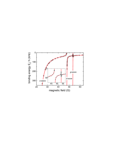
Figure 3: (color online). Binding energy of cesium molecules near three Feshbach resonances as a function of the magnetic field. Zero energy corresponds to two Cs atoms in the absolute hyperfine ground-state sublevel $|F\!=\!3,m_{F}\!=\!3\rangle$. The measurements are shown as open circles. The fit (solid line) is based on Eq. (19), see text. The inset shows an expanded view in the region of the two $d$- and $g$-wave narrow resonances. The error bars refer to the statistical uncertainties.

III.2 Determination of the scattering length

We now convert the binding energy data into scattering length. For Cs atoms, the vdW energy is $E_{\mathrm{vdW,Cs}}=h\times 2.7$ MHz, and the mean scattering length $\bar{a}=95.7a_{B}$. We apply our model in the regime $E_{\rm b}<E_{\mathrm{vdW,Cs}}$ by fitting the binding energy data with Eq. (19) for overlapping resonances. We consider three resonance terms, which correspond to couplings to the $s$-, $d$-, and $g$-wave molecular states. Each term contains three parameters: Feshbach coupling strength $\Gamma_{i}$, bare state crossing position $B_{c,i}$ and the relative magnetic moment $\delta\mu_{i}$ dmub1 . All the parameters are evaluated by the fit. We assign the uncertainties of the parameters by a resampling method resampling . Second, we use the fitting parameters to determine $a$ in the form of Eq. (18). Table 1 summarizes the main fit results for the three overlapping resonances. We derive the zeroes and poles of the scattering length from Eq. (18) and (20). Our results represent the most accurate knowledge of the positions and widths of the two experimental important resonances near 48 and 53 G Knoop2008ooa ; Danzl2008

Table 1: Fitting parameters for the $s$-, $d$- and $g$-wave Feshbach resonances, determining the scattering length in the magnetic field range of interest; see Fig. 3. The background scattering length $a_{\mathrm{bg}}=1875a_{0}$, the mean scattering length of cesium $\bar{a}=95.7~{}a_{B}$ and the bare $s$-wave state magnetic moment $\delta\mu_{1}=2.50\mu_{B}$ dmub1 are set constant. Poles $B_{0,i}$ and zeros $B^{*}_{i}$ of the scattering length are derived, see text. Uncertainties in the parentheses are statistical. The systematic uncertainty of the magnetic field is 10 mG.

res.	$\Gamma_{i}/h$(MHz)	$\delta\mu_{i}/\mu_{B}$	$B_{c,i}$ (G)	$B_{0,i}$ (G)	$B^{*}_{i}$ (G)
$s$-wv.	$11.6(3)$	2.50	19.7(2)	-11.1(6)	18.1(6)
$d$-wv.	$0.065(3)$	1.15(2)	47.962(5)	47.78(1)	47.944(5)
$g$-wv.	$0.0042(6)$	1.5(1)	53.458(3)	53.449(3)	53.457(3)

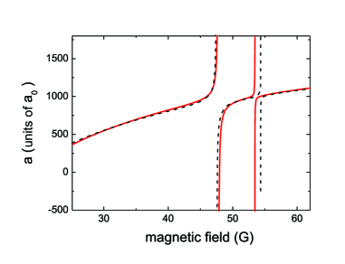
Figure 4: (color online) Scattering length of $|F\!=\!3,m_{F}\!=\!3\rangle$ cesium atoms in the magnetic field range where three Feshbach resonances overlap. The solid curve shows the result of this work while the dashed curve represents the prediction from a previous multi-channel calculation Chin2004 .

Figure 4 shows the magnetic-field dependent scattering length as derived from our model and the binding energy data. We observe a remarkable overall agreement between these results and a previous multi-channel calculation based on the knowledge of the positions of various Feshbach resonances Chin2004 . Our present method proves particularly powerful for the scattering length near the two narrow resonances. Here the previous calculations Chin2004 suffer from the large uncertainties of the positions of the resonances, which can even exceed their widths.

IV Conclusion

In summary, we have described a new method to precisely determine scattering lengths from binding energy measurements of weakly bound molecular states. We employ a simple interaction model to extract the relationship between the scattering length and the binding energy. Using the cesium molecule binding energy data in the range where three Feshbach resonances are present, we show that our model provides an excellent fit to the molecular energy structure, and allows us to precisely determine the scattering length near the resonances. The precise knowledge of binding energy and scattering length near Feshbach resonances provides an ideal starting point to explore few- and many-body physics by controlling the two-body interactions. Our model is also general in the sense that it can apply to any homonuclear or heteronuclear atomic systems near Feshbach resonances, once molecular binding energy data are available.

References

- (1) C. Chin, R. Grimm, P. S. Julienne, and E. Tiesinga, Rev. Mod. Phys. , in preparation.
- (2) E. A. Donley, N. R. Claussen, S. L. Cornish, J. L. Roberts, E. A. Cornell, and C. E. Wieman, Nature 412, 295 (2001).
- (3) T. Köhler, K. Góral, and P. S. Julienne, Rev. Mod. Phys. 78, 1311 (2006).
- (4) F. Ferlaino, S. Knoop, and R. Grimm, Chapter of the Book Cold Molecules: Theory, Experiment, Applications edited by R. V. Krems, B. Friedrich and W. C. Stwalley, arXiv:0809.3920 (2008).
- (5) M. Inguscio, W. Ketterle, and C. Salomon, eds., Ultracold Fermi Gases (IOS Press, Amsterdam, 2008), Proceedings of the International School of Physics Enrico Fermi , Course CLXIV, Varenna, 20-30 June 2006.
- (6) S. Giorgini, L. P. Pitaevskii, and S. Stringari, arXiv:0706.3360 (2007).
- (7) T. Kraemer, M. Mark, P. Waldburger, J. G. Danzl, C. Chin, B. Engeser, A. D. Lange, K. Pilch, A. Jaakkola, H. -C. Nägerl and R. Grimm, Nature 440, 315 (2006).
- (8) C. Chin and V. V. Flambaum, Phys. Rev. Lett. 96, 230801 (2006).
- (9) E. Tiesinga, C. J. Williams, P. S. Julienne, K. M. Jones, P. D. Lett, and W. D. Phillips, J. Res. Nat. Inst. Stand. Technol. 101, 505 (1996).
- (10) E. R. I. Abraham, W. I. McAlexander, J. M. Gerton, R. G. Hulet, R. Côté, and A. Dalgarno, Phys. Rev. A. 55, R3299 (1997).
- (11) A. Marte, T. Volz, J. Schuster, S. Dürr, G. Rempe, E. G. M. van Kempen, and B. J. Verhaar, Phys. Rev. Lett. 89, 283202 (2002).
- (12) C.A. Regal, C. Ticknor, J. L. Bohn, and D. S. Jin, Nature 424, 47 (2003).
- (13) M. Bartenstein, A. Altmeyer, S. Riedl, R. Geursen, S. Jochim, C. Chin, J. H. Denschlag, R. Grimm, A. Simoni, E. Tiesinga, C. J. Williams, and P. S. Julienne, Phys. Rev. Lett. 94, 103201 (2005).
- (14) N. R. Claussen, S. J. J. M. F. Kokkelmans, S. T. Thompson, E. A. Donley, E. Hodby, and C.E. Wieman, Phys. Rev. A 67, 060701(R)(2003).
- (15) S. T. Thompson, E. Hodby, and C. E. Wieman, Phys. Rev. Lett. 95, 190404 (2005).
- (16) S. B. Papp and C. E. Wieman, Phys. Rev. Lett. 97, 180404 (2006).
- (17) C. Chin, V. Vuletić, A. J. Kerman, S. Chu, E. Tiesinga, P. J. Leo, and C. J. Williams, Phys. Rev. A 70, 032701 (2004).
- (18) U. Fano, Phys. Rev. 124, 1866 (1961).
- (19) M. Mark, F. Ferlaino, S. Knoop, J. G. Danzl, T. Kraemer, C. Chin, H. -C. Nägerl, and R. Grimm, Phys. Rev. A 76, 042514 (2007).
- (20) G. F. Gribakin and V. V. Flambaum, Phys. Rev. A 48, 546 (1993).
- (21) J. M. Hutson, E. Tiesinga, and P. S. Julienne, arXiv:0806.2583v1 (2008).
- (22) T. M. Hanna, T. Köhler, and K. Burnett, Phys. Rev. A 75, 013606 (2007).
- (23) D. Rychtarik, B. Engeser, H. -C. Nägerl, and R. Grimm, Phys. Rev. Lett. 92, 173003 (2004).
- (24) The optical trap is formed by a blue-detuned evanescent laser wave (wavelength 810 nm) on top of a horizontal glass prism. In addition a red-detuned laser beam (wavelength 1060 nm, waist 80 m), propagating along the vertical direction, confines the atoms in the horizontal plane.
- (25) S. Knoop, F. Ferlaino, M. Mark, M. Berninger, H. Schöbel, H.-C. Nägerl, and R. Grimm, arXiv:0807.3306v1 (2008).
- (26) J. G. Danzl, E. Haller, M. Gustavsson, M. J. Mark, R. Hart, N. Bouloufa, O. Dulieu, H. Ritsch, and H.-C. Nägerl, Science 321, 1062 (2008).
- (27) C. Chin, T. Kraemer, M. Mark, J. Herbig, P. Waldburger, H. -C. Nägerl, and R. Grimm, Phys. Rev. Lett. 94, 123201 (2005).
- (28) T. Weber, J. Herbig, M. Mark, H. -C. Nägerl, and R. Grimm, Science 232, 232 (2003).
- (29) We use the Breit-Rabi formula to determine the magnetic-field value from a measurement of the resonant frequency corresponding to the atomic hyperfine transition. Line noise limits the stability of the magnetic field to about 10 mG for typical integration times.
- (30) The large uncertainty in fitting the s-wave state magnetic moment leads to an instability of our fitting routine. We remove this instability by assigning Mark2007 .
- (31) We first form subsets of the measurement data (resampling), and then perform the fitting routine. The uncertainties are assigned by analyzing the distribution of the resulting fit parameters. See, for example, P.H. Westfall and S.S. Young, Resampling-based multiple testing, (John Wiley and Sons, New York, 1993).