Two-dimensional quantum random walk

Yuliy Baryshnikov

Wil Brady

Andrew Bressler

Robin Pemantle ^,

ymb@research.bell-labs.com, bradywil@gmail.com,
{bressler,pemantle}@math.upenn.edu

ABSTRACT:
We analyze several families of two-dimensional quantum random walks. The feasible region (the region where probabilities do not decay exponentially with time) grows linearly with time, as is the case with one-dimensional QRW. The limiting shape of the feasible region is, however, quite different. The limit region turns out to be an algebraic set, which we characterize as the rational image of a compact algebraic variety. We also compute the probability profile within the limit region, which is essentially a negative power of the Gaussian curvature of the same algebraic variety. Our methods are based on analysis of the space-time generating function, following the methods of PW [02].

Keywords: Rational generating function, amoeba, saddle point, stationary phase, residue, Fourier-Laplace, Gauss map.

Subject classification: Primary: 05A15, 82C10; Secondary: 41A60.

1 Introduction

1.1 Overview

Quantum random walk, as proposed by ADZ [93], describes the evolution in discrete time of a single particle on the integer lattice. The Hamiltonian is space- and time-invariant. The allowed transitions at each time are a finite set of integer translations. In addition to location, the particle possesses an internal state (the chirality), which is necessary to make the evolution of the location nondeterministic. A rigorous mathematical analysis of this system in one dimension was first given by ABN⁺ [01]. The particle moves ballistically, meaning that at time $n$, its distance from the origin is likely to be of order $n$. By contrast, the classical random walk moves diffusively, being localized to an interval of size $\sqrt{n}$ at time $n$.

A very similar process may be defined in higher dimensions. In particular, given a subset $E\subset{\mathbb{Z}}^{d}$ with cardinality $k$ and a $k\times k$ unitary matrix $U$, there is a corresponding space- and time-homogeneous QRW in which allowed transitions are translations by elements of $E$ and evolution of chirality is governed by $U$. When $E$ is the set of signed standard basis vectors we call this a nearest neighbor QRW; for example in two dimensions, a nearest neighbor walk has $E=\{(0,1),(0,-1),(1,0),(-1,0)\}$; a complete construction of quantum random walk is given in Section 2.1 below. Published work on quantum random walk in dimensions two and higher began around 2002 (see MBSS [02]). Most studies, including the most recent and broad study WKKK [08], are concerned to a great extent with localization; this phenomenon is not generic in quantum random walk models and not present in the models we discuss below. The analyses we have seen range from analytic derivations without complete proofs to numerical studies. As far as we know, no rigorous analysis of two-dimensional QRW has been published. The question of describing the behavior of two-dimensional QRW was brought to our attention by Cris Moore (personal communication). In the present paper, we answer this question by proving theorems about the limiting shape of the feasible region (the region where probabilities do not decay exponentially with time) for two-dimensional QRW, and by giving asymptotically valid formulae for the probability amplitudes at specific locations within this region.

Common to every nondegenerate instance of two-dimensional QRW is ballistic motion with random velocity in some feasible set of velocities, with exponentially decaying probabilities to be found outside the feasible set. The feasible set varies by instance and its shape appears strange and unpredictable. We will show that it is the image of a compact set (a torus) under the logarithmic Gauss map. An explicit description of the feasible set and explicit formulae for probability amplitudes at specific points inside and outside of the feasible set may be obtained; however, these details differ greatly from one instance to another. Because of this, it is difficult to state an omnibus theorem as to asymptotic large-time amplitudes. Instead, we concentrate on three familes of nearest neighbor QRW which together capture all of the qualititative behavior we have seen. These examples also embody all the techniques one would need to analyze other instances. The choice of these particular three families is somewhat of a historical accident, these being one-parameter families of unitary matrices interpolating between various standard unitary matrices (such as Hadamard matrices) which are commonly used and which we first used in numerical experiments. The reason we used one-parameter families was to make animations of the resulting feasible regions as the value of the parameter changed.

1.2 Methods

Our analyses begin with the space-time generating function. This is a multivariate rational function which may be derived without too much difficulty. The companion paper BP [07] introduces this approach and applies it to an arbitrary one-dimensional QRW with two chiralities ($k=2$). This approach allows one to obtain detailed asymptotics such as an Airy-type limit in a scaling window near the endpoints. As such, it improves on the analysis of ABN⁺ [01] but not on the more recent and very nice analysis of CIR [03]. In one dimension, when the number of chiralities exceeds two, N. Konno IKS [05] found new behavior that is qualitatively different from the two-chirality QRW. Forthcoming work of the last author with T. Greenwood uses the generating function approach to greatly extend Konno’s findings.

The generating function approach, however, pays its greatest dividends in dimension two and higher. This approach is based on recent results on asymptotics of multivariate rational generating functions. These results allow nearly automatic transfer from rational generating functions to asymptotic formulae for their coefficients PW [02, 04, 08]; BP [08]. Based on these transfer theorems, analysis of any instance of a two-dimensional QRW becomes relatively easy, with the main technical work being in adaptation of existing methods to more general setting, or in exploiting simplifications arising in cases of interest.

There is, however, a price to pay in terms of overhead: algebraic geometry of the pole variety plays a central role, and one must understand as well the amoeba (domains of convergence of Laurent series), the logarithmic Gauss map, and residue methods in several complex variables. All of this is laid out in PW [02] and PW [04], but these are long and technical. In the present work, we aim to satisfy two audiences: those interested in QRW from the physics or quantum information theory end, who may care much more about results than methods, and those chiefly interested in combinatorial analysis, who are familiar with more standard generating function methods but know little about quantum walks or multivariate generating function analysis. With this in mind, we attempt an explanation of mutlivariate rational generating function analysis that is limited to the cases at hand: functions satisfying the toriality condition of Proposition 2.1. A table of notation appearing at the end of the introduction should enable the reader to skim any parts of the paper focusing on details of less concern.

In the end, we believe that the technical baggage in this paper is worth the price because the results tell a definitive story about QRW in any dimension. No family of QRW in dimension three or higher has been analyzed to date, for example, but such an undertaking should be a modest extension of the present work. Also, the study of bound states in dimensions two and higher should reduce to factorability of the determinant in equation (2.4) below.

1.3 Results

Figure 1a shows the probabilities at time 200 for a particular QRW (one discussed in Section 4.3). Our main goal is to predict and explain such phenomena by computing asymptotic limits. Figure 1b, for example, shows the set of feasible velocities of the same QRW as computed in Theorem 4.9.

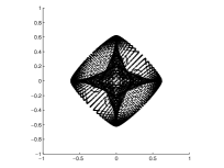
(a) limit

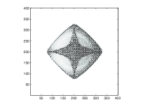
(b) Exact probabilities at time 200

Figure 1: Theoretical limit versus fixed-time empirical plot

To carry this out, we began by computing probability profiles for a number of instances of two-dimensional QRW. The pictures, which appear scattered throughout the paper, are quite varied. Not only did we find these pictures visually intriguing, but they pointed us toward some refinements of the theoretical work in PW [02], which we now describe, beginning with a more detailed description of the two plots.

On the right is depicted the probability distribution for the location of a particle after 200 steps of a quantum random walk on the planar integer lattice; the particular instance of QRW is a nearest neighbor walk ($E=\{(0,1),(0,-1),(1,0),(-1,0)\}$) whose unitary matrix is discussed in Section 4. Greater probabilities are shown as darker shades of grey. The feasible region, where probabilities are not extremely close to zero, appears as a slightly rounded diamond whose vertices if not rounded would be the midpoints of the $400\times 400$ square.

In his Masters Thesis, the second author computed an asymptotically valid formula for the probability amplitudes associated with some instances of QRW. As $n\to\infty$, the probabilities become exponentially small outside of a certain algebraic set ${\bf\Xi}$, but are $\Theta(n^{-2})$ inside of ${\bf\Xi}$. Theorem 4.5 of Bra [07] proves such a shape result for a different instance of two-dimensional QRW and conjectures it for this one, giving the believed characterization of $\Xi$ as an algebraic set. The plot in Figure 1a is a picture of this characterization, constructed by parametrizing $\Xi$ by patches in the flat torus $T_{0}:=({\mathbb{R}}/2\pi{\mathbb{Z}})^{2}$ and then depicting the patches by showing the image of a grid embedded in the torus.

When the plot was constructed, it was intended only to exhibit the overall shape. Nevertheless, it is visually obvious that significant internal structure is duplicated as well. Identical dark regions in the shape of a Maltese cross appear inside each of the two figures. To explain this, we consider the map $\Phi:{\bf T}\to{\mathbb{R}}^{2}$ whose image produces the region $\Xi$, where ${\bf T}$ denotes the unit torus. Let ${\cal V}$ denote the pole variety of the generating function $F$ for a given QRW, that is, the complex algebraic hypersurface on which the denominator $H$ of $F$ vanishes. Let ${\cal V}_{1}$ denote the intersection of ${\cal V}$ with the unit torus ${\bf T}$. It is easy to solve for the third coordinate $z$ as a local function of $x$ and $y$ on ${\cal V}_{1}$ and thereby obtain a piecewise parametrization

$$(\alpha,\beta)\mapsto\left(e^{i\alpha},e^{i\beta},e^{i\phi(\alpha,\beta)}\right)$$

of ${\cal V}_{1}$ by patches in ${\mathbb{R}}^{2}$. Theorem 3.3 extends the results of PW [02] to show that each point ${\bf z}$ of ${\cal V}_{1}$ produces a polynomially decaying contribution to the probability profile for movement at velocity $(r,s)$ which is the image of ${\bf z}$ under the logarithmic Gauss map ${\mathfrak{n}}$ of the surface ${\cal V}_{1}$ at ${\bf z}$:

$${\mathfrak{n}}({\bf z}):=\left(x\frac{\partial H}{\partial x},y\frac{\partial H}{\partial y},z\frac{\partial H}{\partial z}\right)\;.$$ (1.1)

Formally, ${\mathfrak{n}}$ maps into the projective space ${\mathbb{R}}{\mathbb{P}}^{2}$, but we map this to ${\mathbb{R}}^{2}$ by taking the projection $\pi(r,s,t):=(r/t,s/t,1)$. In other words, the plot is the image of the grid $({\mathbb{Z}}/100{\mathbb{Z}})^{2}$ under the following composition of maps:

$${({\mathbb{Z}}/100{\mathbb{Z}})^{2}}\xrightarrow{\iota}S^{1}\times S^{1}\xrightarrow{(1,1,\phi)}{\cal V}\xrightarrow{{\mathfrak{n}}}{\mathbb{R}}{\mathbb{P}}^{2}\xrightarrow{{\pi}}{\mathbb{R}}^{2}\,.$$ (1.2)

The intensity of an image of a uniform grid of dots is proportional to the inverse of the Jacobian of the mapping. The Jacobian of the composition is the product of the Jacobians of the factors, the most significant factor being the Gauss map, ${\mathfrak{n}}$. Its Jacobian is just the Gaussian curvature (in logarithmic coordinates). The darkest regions therefore correspond to the places where the curvature of $\log{\cal V}_{1}$ vanishes. Alignment of this picture with the empirical amplitudes can only mean that the formulae for asymptotics of generating functions given in PW [02] blow up when the Gaussian curvature of $\log{\cal V}_{1}$ vanishes. This observation allowed us to produce new expressions for the quantities in the conclusions of theorems in PW [02], where lengthy polynomials were replaced by quantities involving Gaussian curvatures.

1.4 Summary

To summarize, the purpose of this paper is twofold:

1. In Theorem 4.9, we prove the shape conjecture from Bra [07]; further instances of this are proved in Theorems 4.2 and 4.7.

2. In Theorems 3.3 and 3.5 we reformulate the main result in PW [02] to clarify the relation between the asymptotics of a multivariate rational generating function and the curvature of the pole variety in logarithmic coordinates.

The organization of the remainder of this paper is as follows. Section 2 gives some background on quantum random walks, notions of Gaussian curvature, amoebas of Laurent polynomials, the multivariate Cauchy formula, and certain standard applications of the stationary phase method to the evaluation of oscillating integrals. Section 3 contains general results on rational multivariate asymptotics that will be used in the derivation of the QRW limit theorems. In particular, Theorem 3.3 gives a new formulation of the main result of PW [02], while Theorem 3.5 proves a version of these results in situations where the geometry of ${\cal V}_{1}$ is more complicated than can be handled by the methods of PW [02]. Finally, Section 4 applies these results to a collection of instances of two-dimensional nearest neighbor QRW in which the unitary matrices are elements of one-parameter families named $S(t),A(t)$ and $B(t)$, $0<t<1$. This results in Theorems 4.2, 4.7 and 4.9 respectively. Illustrations of feasible sets for these families of QRW may be found in Section 4.

1.5 Table of notation

Notation	Meaning	Location
$\Xi$	feasible set of velocities	Section 1
${\bf T}_{d},{\bf T}$	unit torus in ${\mathbb{C}}^{d}$	Section 1
${\mathfrak{n}}$	logarithmic Gauss map	Equation (1.1)
$k,E,U,{\bf v}^{(1)},\ldots,{\bf v}^{(k)}$	parameters of a generic QRW	Section 2.1
$M$	diagonal matrix of one-step monomials	Equation (2.2)
F (z)	spacetime generating function	Equation (2.3)
$G/H$	rational function representation of $F$	Equation (2.4)
${\cal V}$	the pole variety, where $H$ vanishes	Proposition 2.2
${\cal V}_{1}$	${\cal V}\cap{\bf T}$	Proposition 2.2, Section 3
${\cal K}$	the Gauss-Kronecker curvature	Equation (2.6)
${\rm Log}\,$	log modulus map	Equation (2.12)
${\nabla_{\rm\log}}$	logarithmic gradient	following Equation (2.14)
${\bf W}({\bf r})$	set of critical points for direction ${\bf r}$	Equation (2.14)
${\cal H}$	Hessian determinant	Equation (2.16)
$\mbox{\rm RES}\,(F\,d{\bf z})$	residue form	Proposition 3.1
the superscript $\circ$	homogeneous part	Equation (3.7)
$B_{0}$	log-domain for the Laurent series $F$	Section 2.3
${\bf K}$	dual cone to $B_{0}$ at ${\bf 0}$	preceding Theorem 3.3
${\cal W}$	the singular subset of ${\cal V}_{1}$	Section 3
${\cal G}$	the image ${\mathfrak{n}}[{\cal V}_{1}\setminus{\cal W}]$	Section 4

2 Preliminaries

2.1 Quantum random walks

The quantum random walk is a model for the motion of a single quantum particle evolving in ${\mathbb{Z}}^{d}$ under a time and translation invariant Hamiltonian for which the probability profile of a particle after one time step, started from a known location, is uniform on the neighbors. Such a process was first constructed in ADZ [93]. Let $d\geq 1$ be the spatial dimension. Let $E=\{{\bf v}^{(1)},\ldots,{\bf v}^{(k)}\}\subseteq{\mathbb{Z}}^{d}$ be a set of finite cardinality $k$. Let $U$ be a unitary matrix of size $k$. The set ${\mathbb{Z}}^{d}\times E$ indexes the set of pure states of the QRW with parameters $k,E$ and $U$; the set of all states is the unit ball in $L^{2}({\mathbb{Z}}^{d}\times E)$; the parameter $k$ is somewhat redundant, being the cardinality of $E$, but it seems clearer to leave it in the notation. Let ${\rm Id}\otimes U$ denote the operator that sends $({\bf r},{\bf v}^{(j)})$ to $({\bf r},U{\bf v}^{(j)})$, that is, it leaves the location unchanged but operates on the chirality by $U$. Let $\sigma$ denote the operator that sends $({\bf r},{\bf v}^{(j)})$ to $({\bf r}+{\bf v}^{(j)},{\bf v}^{(j)})$, that is, it translates the location according to the chirality and does not change the chirality. The product $\sigma\cdot({\rm Id}\otimes U)$ is the operator we call QRW with parameters $k,E$ and $U$. Let us denote this by ${\cal Q}$.

For $1\leq i,j\leq k$ and ${\bf r}\in{\mathbb{Z}}^{k}$,

$$\psi_{n}^{(i,j)}{\bf r}:=\langle e_{{\bf 0},i}|{\cal Q}^{n}|e_{{\bf r},j}\rangle$$

denotes the amplitude at time $n$ for a particle starting at location ${\bf 0}$ in chirality $i$ to be in location ${\bf r}$ and chirality $j$. For combinatorial readers of this paper, we point out that the notation $({\bf v}|A|{\bf v})$ is the traditional physicist’s notation for ${\bf v}^{T}A{\bf v}$ and that the amplitude is a quantum quantity whose square modulus is interpreted as the probability of the transition in question (i.e., of a transition from $({\bf 0},i)$ to $({\bf r},j)$ in $n$ steps).

Let ${\bf z}$ denote $(z_{1},\ldots,z_{d+1})$ and define

$$F^{(i,j)}({\bf z}):=\sum_{n,{\bf r}}\psi_{n}^{(i,j)}({\bf r})z_{1}^{r_{1}}\cdots z_{d}^{r_{d}}z_{d+1}^{n}$$ (2.1)

which denotes the spacetime generating function for $n$-step transitions from chirality $i$ to chirality $j$ and all locations. Let ${\bf F}({\bf z})$ denote the matrix $(F^{(i,j)})_{1\leq i,j\leq k}$. Let $M$ denote the diagonal matrix whose entries are the monomials $\{{\bf z}^{{\bf v}^{(j)}}:1\leq j\leq k\}$. When $d=2$ we use $(x,y,z)$ for $(z_{1},z_{2},z_{3})$ and $(r,s)$ for ${\bf r}$; for a two-dimensional nearest neighbor QRW, therefore, the notation becomes

$$F^{(i,j)}(x,y,z)=\sum_{n,r,s}\psi_{n}^{(i,j)}(r,s)x^{r}y^{s}z^{n}$$

and

$$M=\left(\begin{array}[]{cccc}x&0&0&0\\ 0&x^{-1}&0&0\\ 0&0&y&0\\ 0&0&0&y^{-1}\end{array}\right)\;.$$ (2.2)

An explicit expression for ${\bf F}$ may be derived via an elementary enumerative technique known as the transfer matrix method Sta [97]; GJ [83]. For $d=1$ and a particular choice of $U$ (the Hadamard matrix), this rational function is computed in ABN⁺ [01]. In [BP, 07, Section 3], the following formula is given for the matrix generating function ${\bf F}$, representing a Laurent series convergent in an annulus $\{(z_{1},\ldots,z_{d+1}):(\log|z_{1}|,\ldots,\log|z_{d+1}|)\in R$ for some convex region $R$:

$${\bf F}({\bf z})=\left(I-z_{d+1}MU\right)^{-1}\,.$$ (2.3)

The $(i,j)$-entry of the matrix, $F^{(i,j)}$, may therefore be written as a rational function $G/H$ where

$$H=\det(I-z_{d+1}MU)\,.$$ (2.4)

The following result is easy but crucial. It is valid in any dimension $d\geq 1$. Let ${\bf T}_{d}$ denote the unit torus in ${\mathbb{C}}^{d}$.

Proposition 2.1 (torality).

The denominator $H$ of the spacetime generating function for a quantum random walk has the property that

$$(z_{1},\ldots,z_{d})\in{\bf T}_{d}\mbox{ and }H({\bf z})=0\;\;\Longrightarrow\;\;|z_{d+1}|=1\,.$$ (2.5)

Proof: If $(z_{1},\ldots,z_{d})\in{\bf T}_{d}$ then $M$ is unitary, hence $MU$ is unitary. The zeros of $\det(I-z_{d+1}MU)$ are the reciprocals of eigenvalues of $MU$, which are therefore complex numbers of unit modulus. $\hfill\Box$

Proposition 2.2.

Let $H$ be any polynomial and let ${\cal V}$ denote the pole variety, namely the set $\{{\bf z}:H({\bf z})=0\}$. Let ${\cal V}_{1}:={\cal V}\cap{\bf T}_{d+1}$. Assume the torality hypothesis (2.5). Let $p\in{\cal V}_{1}$ be any point for which $\nabla H(p)\neq{\bf 0}$. Then ${\cal V}_{1}$ is a smooth $d$-dimensional manifold in a neighborhood of $p$.

Proof: We will show that $\partial H/\partial z_{d+1}(p)\neq 0$. It follows by the implicit function theorem that there is an analytic function $g:{\mathbb{C}}^{d}\to{\mathbb{C}}$ such that for ${\bf z}$ in some neighborhood of $p$, $H({\bf z})=0$ if and only if $z_{d+1}=g(z_{1},\ldots,z_{d})$. Restricting $(z_{1},\ldots,z_{d})$ to the unit torus, the torality hypothesis implies $|z_{d+1}|=1$, whence ${\cal V}_{1}$ is locally the graph of a smooth function.

To see that $\partial H/\partial z_{d+1}(p)\neq 0$, first change coordinates to $z_{j}=p_{j}\exp(i\theta_{j})$ and $z_{d+1}=p_{d+1}\exp(is)$. Letting $\tilde{H}:=H\circ\exp$, the new torality hypothesis is $(\theta_{1},\ldots,\theta_{d})\in{\mathbb{R}}^{d}$ and $H(\theta_{1},\ldots,\theta_{d},s)=0$ implies $s\in{\mathbb{R}}$. We are given $\nabla\tilde{H}({\bf 0})\neq{\bf 0}$ and are trying to show that $\partial\tilde{H}/\partial s({\bf 0})\neq 0$.

Consider first the case $d=1$ and let $\theta:=\theta_{1}$. Assume for contradiction that $\partial\tilde{H}/\partial s(0,0)=0\neq\partial\tilde{H}/\partial\theta(0,0)$. Let $\tilde{H}(\theta,s)=\sum_{j,k\geq 0}b_{j,k}\theta^{j}s^{k}$ be a series expansion for $\tilde{H}$ in a neighborhood of $(0,0)$. We have $b_{0,0}=0\neq b_{1,0}$. Let $\ell$ be the least positive integer for which the $b_{0,\ell}\neq 0$; such an integer exists (otherwise $\tilde{H}(0,s)\equiv 0$, contradicting the new torality hypothesis) and is at least 2 by the vanishing of $\partial H/\partial s(0,0)$. Then there is a Puiseux expansion for the curve $\{\tilde{H}=0\}$ for which $s\sim(-b_{1,0}\theta/b_{0,\ell})^{1/\ell}$. This follows from BK [86] although it is quite elementary in this case: as $s,\theta\to 0$, the power series without the $(1,0)$ and $(0,\ell)$ terms sums to $O(|\theta|^{2}+|\theta s|+|s|^{\ell+1})=o(|\theta|+|s|^{\ell})$ (use Hölder’s inequality); in order for $\tilde{H}$ to vanish, one must therefore have $b_{1,0}\theta+b_{0,\ell}s^{\ell}=o(|\theta|+|s|^{\ell})$, from which $s\sim(-b_{1,0}\theta/b_{0,\ell})^{1/\ell}$ follows. The only way the new torality hypothesis can now be satisfied is if $\ell=2$ and $b_{1,0}\theta/b_{0,\ell}$ does not change sign; but $\theta$ may take either sign, so we have a contradiction.

Finally, if $d>1$, again we must have $b_{0,\ldots,0,\ell}\neq 0$ in order to avoid $\tilde{H}(0,\ldots,0,s)\equiv 0$. Proceeding again by contradiction, we let ${\bf r}\in{\mathbb{R}}^{d+1}$ be any vector not orthogonal to $\nabla\tilde{H}({\bf 0})$ and let $G(\theta,s):=\tilde{H}(r_{1}\theta,\ldots,r_{d}\theta,s)$. Then $\partial G/\partial\theta(0,0)\neq 0=\partial G/\partial s(0,0)$ and the new torality hypothesis holds for $G$; a contradiction then results from the above analysis for the case $d=1$. $\hfill\Box$

A Hadamard matrix is one whose entries are all $\pm 1$. There is more than one rank-4 unitary matrix that is a constant multiple of a Hadamard matrix, but for some reason the “standard Hadamard” QRW in two dimensions is the QRW whose unitary matrix is

$$U_{\rm Had}:=\frac{1}{2}\left(\begin{array}[]{cccc}1&-1&-1&-1\\ -1&1&-1&-1\\ -1&-1&1&-1\\ -1&-1&-1&1\end{array}\right)\,.$$

This is referred to by Konno IKK [04]; WKKK [08] as the “Grover walk” because of its relation to the quantum search algorithm of L. Grover Gro [96]. Shown in Figure 2b is a plot of the probability profile for the position of a particle performing a standard Hadamard QRW for 200 time steps. This is the only two-dimensional QRW we are aware of for which even a nonrigorous analysis had previously been carried out. On the left, in Figure 2a, is the analogous plot of the region of non-exponential decay.

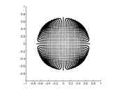
(a) limit

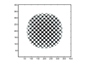
(b) exact probabilities at time 200

Figure 2: Moore’s Hadamard QRW

Another $4\times 4$ unitary Hadamard matrix reflects the symmetries of $({\mathbb{Z}}/(2{\mathbb{Z}}))^{2}$ rather than ${\mathbb{Z}}/(4{\mathbb{Z}})$:

$$\tilde{U}_{\rm Had}:=\frac{1}{2}\left(\begin{array}[]{cccc}1&1&1&1\\ -1&1&-1&1\\ 1&-1&-1&1\\ -1&-1&1&1\end{array}\right)\,.$$

This matrix also goes by the name of $S(1/2)$ and is a member of the first family of QRW that we will analyze. There is no reason to stick with Hadamard matrices. Varying $U$ further produces a number of other probability profiles including the families $S(t),A(t)$ and $B(t)$ analyzed in Section 4.

2.2 Differential Geometry

For a smooth orientable hypersurface ${\cal V}\subset{\mathbb{R}}^{d+1}$, the Gauss map ${\mathfrak{n}}$ sends each point $p\in{\cal V}$ to a consistent choice of normal vector. We may identify ${\mathfrak{n}}(p)$ with an element of $S^{d}$. For a given patch $P\subset{\cal V}$ containing $p$, let ${\mathfrak{n}}[P]:=\cup_{q\in P}{\mathfrak{n}}(q)$, and denote the area of a patch $P$ in either ${\cal V}$ or $S^{d}$ as $A[P]$. Then the Gauss-Kronecker curvature of ${\cal V}$ at $p$ is defined as (see the diffgeom wiki or, e.g., [GP, 74, page 195])

$${\cal K}:=\lim_{P\rightarrow p}\frac{A({\mathfrak{n}}[P])}{A[P]}\,.$$ (2.6)

When $d$ is odd, the antipodal map on $S^{d}$ has determinant $-1$, whence the particular choice of unit normal will influence the sign of ${\cal K}$, which is therefore only well defined up to sign. When $d$ is even, we take the numerator to be negative if the map ${\mathfrak{n}}$ is orientation reversing and we have a well defined signed quantity. Clearly, ${\cal K}$ is equal to the Jacobian of the Gauss map at the point $p$. For computational purposes, it is convenient to have a formula for the curvature of the graph of a function from ${\mathbb{R}}^{d}$ to ${\mathbb{R}}$.

Proposition 2.3.

Suppose that in a neighborhood of the point $p$, the smooth hypersurface ${\cal V}\subseteq{\mathbb{R}}^{d+1}$ is the graph of a smooth function, that is for some neightborhood ${\cal N}$ of ${\bf 0}$ in ${\mathbb{R}}^{d}$ and some smooth $h:{\cal N}\to{\mathbb{R}}$ mapping ${\bf 0}$ to 0, ${\cal V}=\{p+({\bf x},\tau):\tau=h({\bf x})\}$. Let $\nabla:=\nabla h({\bf 0})$ and $\displaystyle{{\cal H}:=\det\left(\frac{\partial h}{\partial u_{i}\partial u_{j}}({\bf 0})\right)_{1\leq i,j\leq d}}$ denote respectively the gradient and Hessian determinant of $h$ at the origin. Then the curvature of ${\cal V}$ at $p$ is given by

$${\cal K}=\frac{{\cal H}}{\sqrt{1+|\nabla|^{2}}^{\,2+d}}\,.$$

The square root is taken to be positive and in case $d$ is odd, the curvature is with respect to a unit normal in the direction in which the dependent variable increases.

Proof: Translating by $p$ if necessary, we may assume without loss of generality that $p$ is the origin. Let $\bf{X}:U\subseteq{\mathbb{R}}^{d}\to{\mathbb{R}}^{d+1}$ denote the parametrizing map defined by

$${\bf X}({\bf u}):=(u_{1},\ldots,u_{d},h(u_{1},\ldots,u_{d}))$$

on a neighborhood $U$ of the origin. Let $\pi$ be the restriction to ${\cal V}$ of projection of ${\mathbb{R}}^{d+1}$ onto the first $d$ coordinates, so $\pi$ inverts $\bf{X}$ on $U$. Define a vector

$${\bf N}({\bf u}):=\left(\frac{\partial h}{\partial u_{1}},\ldots,\frac{\partial h}{\partial u_{d}},-1\right)$$

normal to ${\cal V}$ at $\bf{X}({\bf u})$ and let ${\hat{{\bf N}}}$ denote the corresponding unit normal ${\bf N}/|{\bf N}|$. Observe that $|{\bf N}|=\sqrt{1+|\nabla h|^{2}}$, and in particular, that $|{\bf N}({\bf 0})|=\sqrt{1+|\nabla|^{2}}$. The Jacobian of $\pi$ at the point $p$ is, up to sign, the cosine of the angle between the $z_{d+1}$ axis and the normal to the tangent plane to ${\cal V}$ at $p$. Thus

$$|J(\pi(p))|=\frac{|{\hat{{\bf N}}}\cdot e_{d+1}|}{|{\hat{{\bf N}}}||e_{d+1}|}=\frac{1/|{\bf N}({\bf 0})|}{1\cdot 1}=\frac{1}{\sqrt{1+|\nabla|^{2}}}\,.$$ (2.7)

The Gaussian curvature at the point $p$ is (up to sign), by definition, the Jacobian of the map ${\hat{{\bf N}}}\circ\pi$ at $p$. Using $J$ to denote the Jacobian, write ${\hat{{\bf N}}}$ as $|\cdot|\,\circ{\bf N}$ and apply the chain rule to see that

$${\cal K}=J(\pi(p))\cdot J({\bf N})({\bf 0})\cdot J(|\cdot|\,)({\bf N}({\bf 0}))\;=\frac{1}{\sqrt{1+|\nabla|^{2}}}\cdot J({\bf N})({\bf 0})\cdot J(|\cdot|\,)(\nabla,-1)\,.$$ (2.8)

Here, $|\cdot|\,$ is considered as a map from ${\mathbb{R}}^{d}\times\{-1\}$ to $S^{d}$; at the point ${\bf y}$, its differential is an orthogonal projection onto the plane orthogonal to $({\bf y},-1)$ times a rescaling by $|({\bf y},-1)|^{-1}$, whence

$$J(|\cdot|\,)({\bf y})=\sqrt{1+|{\bf y}|^{2}}^{\,-1}\sqrt{1+|{\bf y}|^{2}}^{\,-d}\,.$$ (2.9)

Because ${\bf N}$ maps into the plane $z_{d+1}=-1$ we may compute $J({\bf N})$ from the partial derivatives $\partial N_{i}/\partial x_{j}=\partial^{2}h/\partial x_{i}\partial x_{j}$, leading to $J({\bf N})({\bf 0})={\cal H}$. Putting this together with (2.9) gives

$$J({\hat{{\bf N}}})({\bf 0})=\frac{{\cal H}}{\sqrt{1+|\nabla|^{2}}^{\,d+1}}$$ (2.10)

and using (2.8) and (2.7) gives

$${\cal K}=\frac{{\cal H}}{\sqrt{1+|\nabla|^{2}}^{\,d+2}}\,,$$

proving the proposition. $\hfill\Box$

We pause to record two special cases, the first following immediately from $\nabla h({\bf 0})={\bf 0}$. If $Q$ is a homogeneous quadratic form, we let $||Q||$ denote the determinant of the Hessian matrix of $Q$; to avoid confusion, we point out that the diagonal elements $q_{ii}$ of this matrix are twice the coefficient of $x_{i}^{2}$ in $Q$. The determinant will be the same when the coefficients of $||Q||$ may be computed with respect to any orthonormal basis.

Corollary 2.4.

Let ${\cal P}$ be the linear subspace such that $p+{\cal P}$ is tangent to ${\cal V}$ at $p$ and let ${\bf v}$ be a unit normal. Suppose that ${\cal V}$ is the graph of a smooth function $h$ over ${\cal P}$, that is,

$${\cal V}=\{p+{\bf u}+h({\bf u}){\bf v}:{\bf u}\in U\subseteq{\cal P}\}\,.$$

Let $Q$ be the quadratic part of $h$, that is, $h({\bf u})=Q({\bf u})+O(|{\bf u}|^{3})$. Then the curvature of ${\cal V}$ at $p$ is given by

$${\cal K}=||Q||\,.$$

$\hfill\Box$

Corollary 2.5 (curvature of the zero set of a polynomial).

Suppose ${\cal V}$ is the set $\{{\bf x}:H({\bf x})=0\}$ and suppose that $p$ is a smooth point of ${\cal V}$, that is, $\nabla H(p)\neq{\bf 0}$. Let $\nabla$ and $Q$ denote respectively the gradient and quadratic part of $H$ at $p$. Let $Q_{\perp}$ denote the restriction of $Q$ to the hyperplane $\nabla_{\perp}$ orthogonal to $\nabla$. Then the curvature of ${\cal V}$ at $p$ is given by

$${\cal K}=\frac{||Q_{\perp}||}{|\nabla|^{d}}\,.$$ (2.11)

Proof: Replacing $H$ by $|\nabla|^{-1}H$ leaves ${\cal V}$ unchanged and reduces to the case $|\nabla H(p)|=1$; we therefore assume without loss of generality that $|\nabla|=1$. Letting ${\bf u}_{\perp}+\lambda({\bf u})\nabla$ denote the decomposition of a generic vector ${\bf u}$ into components $\nabla_{\perp}$ and $\langle\nabla\rangle$, the Taylor expansion of $H$ near $p$ is

$$H(p+{\bf u})=\nabla\cdot{\bf u}+Q_{\perp}({\bf u})+R$$

where $R=O(|{\bf u}_{\perp}|^{3}+|\lambda({\bf u})||{\bf u}_{\perp}|)$. Near the origin, we solve for $\lambda$ to obtain a parametrization of ${\cal V}$ by $\nabla_{\perp}$:

$$\lambda({\bf u})=Q_{\perp}({\bf u})+O(|{\bf u}|^{3})\,.$$

The result now follows from the previous corollary. $\hfill\Box$

2.3 Amoebae and Cauchy’s formula

Let $F=G/H$ be a quotient of Laurent polynomials, with pole variety ${\cal V}:=\{{\bf z}:H({\bf z})=0\}$. Let ${\rm Log}\,:({\mathbb{C}}^{*})^{d+1}\to{\mathbb{R}}^{d+1}$ denote the log-modulus map, defined by

$${\rm Log}\,({\bf z}):=(\log|z_{1}|,\ldots,\log|z_{d+1}|)\,.$$ (2.12)

The amoeba of $H$ is defined to be the image under ${\rm Log}\,$ of the variety ${\cal V}$. To each component $B$ of the complement of this amoeba in ${\mathbb{R}}^{d+1}$ corresponds to a Laurent series expansion of $F$. When $F$ is the $(d+1)$-variable spacetime generating function of a $d$-dimensional QRW, we will be interested in the component $B_{0}$ containing a translate of the negative $z_{d+1}$-axis; this corresponds to the Laurent expansion that is an ordinary series in the time variable and a Laurent series in the space variables. For QRW, the point ${\bf 0}$ is always on the boundary of $B_{0}$. In general, all components of the complement of any amoeba are convex. For further details and properties of amoebas, see [GKZ, 94, Chapter 6].

For any ${\bf r}\in{\mathbb{R}}^{d+1}$, let $\hat{{\bf r}}$ denote the unit vector ${\bf r}/|{\bf r}|$. Two important hypotheses that will be satisfied for QRW are as follows.

$$\mbox{ The function }{\bf x}\mapsto{\bf r}\cdot{\bf x}\mbox{ is maximized over }\overline{B_{0}}\mbox{ at a specified point }{\bf x}_{*}\,;$$ (2.13)

we will be primarily concerned with those $\hat{{\bf r}}$ for which this maximizing point is the origin, and we denote by ${\bf K}$ the set of $\hat{{\bf r}}$ for which this holds: thus for $\hat{{\bf r}}\in{\bf K}$ and ${\bf x}\in\overline{B_{0}}$, ${\bf r}\cdot{\bf x}\leq 0$ with equality when ${\bf x}={\bf 0}$. Secondly, we assume that

The set ${\bf W}={\bf W}({\bf r})$ of ${\bf z}=\exp({\bf x}+i{\bf y})$ such that

$$H({\bf z})=0\mbox{ and }{\nabla_{\rm\log}}H({\bf z})\parallel\hat{{\bf r}}$$ (2.14)

is finite.

The set ${\bf W}({\bf r})$ depends on ${\bf r}$ only through $\hat{{\bf r}}$. The gradient of $H\circ\exp$ at the point ${\bf z}\in{\bf W}$ is equal to $(z_{1}\partial H/\partial z_{1},\ldots,z_{d+1}\partial H/\partial z_{d+1})$ and will be denoted ${\nabla_{\rm\log}}H({\bf z})$. It is immediate from (2.14) that ${\nabla_{\rm\log}}H({\bf z})$ is a multiple of the real vector ${\bf r}$.

Before we proceed we point out a condition under which (2.14) is always satisfied. Suppose that ${\cal V}_{1}$ is smooth off a finite set ${\cal W}$, and we let ${\bf r}$ be some direction such that hypothesis (2.14) fails. The set ${\bf W}({\bf r})$ is algebraic, so if it is infinite it contains a curve, which is a curve of constancy for the logarithmic Gauss map. This implies that the Jacobian of the logarithmic Gauss map vanishes on the curve, which is equivalent to vanishing Gaussian curvature at every point of the curve. Thus, if we restrict ${\bf r}$ to the subset of ${\cal V}_{1}$ where ${\cal K}\neq 0$, then hypothesis (2.14) is automatically satisfied.

The coefficients $a_{\bf r}$ of the Laurent series corresponding to $B_{0}$ may be computed via Cauchy’s integral formula. Define the flat torus $T_{0}:=({\mathbb{R}}/(2\pi{\mathbb{Z}}))^{d+1}$. The following proposition is well known.

Proposition 2.6 (Cauchy’s Integral Formula).

For any ${\bf u}$ interior to $B_{0}$,

$$a_{\bf r}=\left(\frac{1}{2\pi}\right)^{d+1}\exp(-{\bf r}\cdot{\bf u})\int_{T_{0}}\exp(-i{\bf r}\cdot{\bf y})F\circ\exp({\bf u}+i{\bf y})\,d{\bf y}\,.$$ (2.15)

Corollary 2.7.

Let $\lambda:=\lambda(\hat{{\bf r}}):=\sup\{\hat{{\bf r}}\cdot{\bf x}:{\bf x}\in B_{0}\}$. For any $\lambda^{\prime}<\lambda$, the estimate

$$|a_{{\bf r}^{\prime}}|=o(\exp(-\lambda^{\prime}|{\bf r}^{\prime}|))$$

holds uniformly as ${\bf r}^{\prime}\to\infty$ in some cone with ${\bf r}$ in its interior.

Proof: Pick ${\bf u}$ interior to $B_{0}$ such that ${\bf r}\cdot{\bf u}>\lambda^{\prime}$. There is some $\epsilon>0$ and some cone ${\bf K}$ with ${\bf r}$ in its interior such that ${\bf r}^{\prime}\cdot{\bf u}\geq\lambda^{\prime}+\epsilon$ for all ${\bf r}^{\prime}\in{\bf K}$. The function $F$ is bounded on the torus $\exp({\bf u}+i{\bf y})$, and the corollary follows from Cauchy’s formula. $\hfill\Box$

Note: We allow for the possibility that hypothesis (2.14) holds for no points with modulus $1$. In the asymptotic estimate (3.6) below, the sum will be empty and we will be able to conclude that $a_{{\bf r}}=O(|{\bf r}|^{-(d+1)/2})$, as opposed to $\Theta(|{\bf r}|^{-d/2})$ in the more interesting regime; we will not be able to conclude that $a_{{\bf r}}$ decays exponentially, as it does when ${\bf r}\notin\overline{{\bf K}}$. This will correspond to the case where in fact ${\bf r}\in\overline{{\bf K}}\setminus{\bf K}$.

2.4 Oscillating integrals

Let ${\cal M}$ be an oriented $d$-manifold, let $\phi:{\cal M}\to{\mathbb{R}}$ be a smooth function and let $A$ be a smooth $d$-form on ${\cal M}$. Say that $p_{*}\in{\cal M}$ is a critical point for $\phi$ if $d\phi(p_{*})=0$. Equivalently, in coordinates, $p_{*}$ is critical if the gradient vector $\nabla\phi(p_{*})$ vanishes. At a critical point, $\phi(p)-\phi(p_{*})$ is a smooth function of $p$ which vanishes to order at least 2 at $p=p_{*}$. Say that a critical point $p_{*}$ for $\phi$ is quadratically nondegenerate if the quadratic part is nondegenerate; in coordinates, this means that the Hessian matrix

$${\cal H}(\phi;p_{*}):=\left(\frac{\partial^{2}\phi}{\partial x_{i}\partial x_{j}}(p_{*})\right)_{1\leq i,j\leq k}$$ (2.16)

has nonzero determinant. It is well known (e.g., BH [86]; Won [89]) that the integral $\int_{{\cal M}}\exp(i\lambda\phi({\bf y}))A({\bf y})\,d{\bf y}$ can be asymptotically estimated via a stationary phase analysis. The following formulation is adapted from Ste [93].

If $p\mapsto(x_{1},\ldots,x_{d})$ is a local right-handed coordinatization, we denote by $\eta[p,d{\bf x}]$ the value $A(p)$ for the function $A$ such that $\eta=A(p)\,d{\bf x}$. If the real matrix $M$ has nonvanishing real eigenvalues, we denote a signature function $\sigma(M):=n_{+}(M)-n_{-}(M)$ where $n_{+}(M)$ (respectively $n_{-}(M)$) denotes the number of positive (respectively negative) eigenvalues of $M$. Given $\phi$ and $\eta$ as above, and a critical point $p_{*}$ for $\phi$, we claim that the quantity ${\cal F}$ defined by

$${\cal F}(\phi,\eta,p_{*}):=e^{-i\pi\sigma/4}\left|\det{\cal H}(\phi;p_{*})\right|^{-1/2}\eta[p_{*},d{\bf x}]$$ (2.17)

does not depend on the choice of coordinatization. To see this, note that the symmetric matrix ${\cal H}$ has nonzero real eigenvalues, whence $i{\cal H}$ has purely imaginary eigenvalues and the quantity $e^{-i\pi\sigma/4}|\det{\cal H}(\phi;p_{*})|^{-1/2}$ is a $-1/2$ power of $\det(i{\cal H})$, in particular, the product of the reciprocals of the principal square roots of the eigenvalues. Up to the sign choice, this is invariant because a change of coordinates with Jacobian $J$ at $p_{*}$ divides $\eta[p_{*},d{\bf x}]$ by $J$ and ${\cal H}(\phi;p_{*})$ by $J^{2}$. Invariance of the sign choice follows from connectedness of the special orthogonal group, implying that any two right-handed coordinatizations are locally homotopic and the sign choice, being continuous, must be constant.

Lemma 2.8 (nondegenerate stationary phase integrals).

Let $\phi$ be a smooth function on a $d$-manifold ${\cal M}$ and let $\eta$ be a smooth, compactly supported $d$-form on ${\cal M}$. Assume the following hypotheses.

1. The set ${\bf W}$ of critical points of $\phi$ on the support of $\eta$ is finite and non-empty.

2. $\phi$ is quadratically nondegenerate at each $p_{*}\in{\bf W}$.

Then

$$\int_{{\cal M}}\exp(i\lambda\phi)\,\eta=\left(\frac{2\pi}{\lambda}\right)^{d/2}\sum_{p_{*}\in{\bf W}}e^{i\lambda\phi(p_{*})}{\cal F}(\phi,\eta,p_{*})+O\left(\lambda^{-(d+1)/2}\right)\,.$$ (2.18)

Remarks.

The stationary phase method actually gives an infinite asymptotic development for this integral. In our application, the contributions of order $\lambda^{-d/2}$ will not cancel, in which case (2.18) gives an asymptotic formula for the integral. The remainder term (see Ste [93]) is bounded by a polynomial in the reciprocals of $|\nabla\phi|$ and $\det{\cal H}$ and partial derivatives of $\phi$ (to order two) and $\eta$ (to order one); it follows that the bound is uniform if $\phi$ and $\eta$ vary smoothly with $(i)$ and $(ii)$ always holding.

Proof: Let $\{{\cal N}_{\alpha}\}$ be a finite cover of ${\cal M}$ by open sets containing at most one critical point of $\phi$, with each ${\cal N}_{\alpha}$ covered by a single chart map and no two containing the same critical point. Let $\{\psi_{\alpha}\}$ be a partition of unity subordinate to $\{{\cal N}_{\alpha}\}$. Write

$$I:=\int_{{\cal M}}\exp(i\lambda\phi)\,\eta$$

as $\sum_{\alpha}I_{\alpha}$ where

$$I_{\alpha}:=\int_{{\cal N}_{\alpha}}\exp(i\lambda\phi)\,\eta\,\psi_{\alpha}\,.$$

According to [Ste, 93, Proposition 4 of VIII.2.1], when ${\cal N}_{\alpha}$ contains no critical point of $\phi$ then $I_{\alpha}$ is rapidly decreasing, i.e, $I_{\alpha}(\lambda)=o(\lambda^{-N})$ for every $N$. According to [Ste, 93, Proposition 6 of VIII.2.3], when ${\cal N}_{\alpha}$ contains a single nondegenerate critical point $p_{*}$ for $\phi$ then, using the fact that $\psi_{\alpha}(p_{*})=1$,

$$I_{\alpha}=\left(\frac{2\pi}{\lambda}\right)^{d/2}A(p_{*})\prod_{j=1}^{d}\mu_{j}^{-1/2}+O\left(\lambda^{-d/2-1}\right)$$

where $\eta=A({\bf x})d{\bf x}$ in the local chart map, $\{\mu_{j}\}$ are the eigenvalues of $i{\cal H}$ in this chart map, and the principal $-1/2$ powers are chosen. Summing over $\alpha$ then proves the lemma. $\hfill\Box$

As a corollary, we derive the asymptotics for the Fourier transform of a smooth $d$-form on an oriented $d$-manifold immersed in ${\mathbb{R}}^{d+1}$. Let ${\cal M}$ be such a manifold and let ${\cal K}(p)$ denote the curvature of ${\cal M}$ at $p$. If $\eta$ is a smooth, compactly supported $d$-form on ${\cal M}$, denote $\eta[p]=\eta[p,d{\bf x}]$ with respect to the immersion coordinates, and define the Fourier transform $\hat{\eta}$ by

$$\hat{\eta}({\bf r}):=\int_{{\cal M}}e^{i\hat{{\bf r}}\cdot{\bf x}}\cdot\eta\,.$$

Corollary 2.9.

Let $K$ be a compact subset of the unit sphere. Assume that for $\hat{{\bf r}}\in K$, the set ${\bf W}$ of critical points for the phase function $\hat{{\bf r}}\cdot{\bf x}$ is finite (possibly empty), and all critical points are quadratically nondegenerate. For ${\bf x}\in{\bf W}$, let $\tau({\bf x})$ denote the index of the critical point, that is, the difference between the dimensions of the positive and negative tangent subspaces for the function $\hat{{\bf r}}\cdot{\bf x}$. Then

$$\hat{\eta}({\bf r})=\left(\frac{2\pi}{|{\bf r}|}\right)^{d/2}\sum_{{\bf x}_{*}\in{\bf W}}e^{i{\bf r}\cdot{\bf x}_{*}}\eta[{\bf x}_{*}]{\cal K}({\bf x}_{*})^{-1/2}e^{-i\pi\tau({\bf x}_{*})/4}+O\left(\lambda^{-(d+1)/2}\right)$$

uniformly as $|{\bf r}|\to\infty$ with $\hat{{\bf r}}\in K$.

Proof: Plugging $\phi=\hat{{\bf r}}\cdot{\bf x}$ into Lemma 2.8, and comparing with (2.17) we see that we need only to verify for each ${\bf x}_{*}\in{\bf W}$ that

$$e^{-i\pi\sigma/4}\left|\det{\cal H}(\phi;{\bf x}_{*})\right|^{-1/2}\eta[{\bf x}_{*},d{\bf x}]=\eta[{\bf x}_{*}]\left|{\cal K}({\bf x}_{*})\right|^{-1/2}e^{-i\pi\tau({\bf x}_{*})/4}\,.$$

With the immersed coordinates, $\sigma=\tau$, and this amounts to verifying that $|\det{\cal H}(\phi;{\bf x}_{*})|=|{\cal K}({\bf x}_{*})|$. Let ${\cal P}$ denote the tangent space to ${\cal M}$ at ${\bf x}_{*}$ and let $u_{1},\ldots,u_{d}$ be an orthonormal basis for ${\cal P}$. Let $v$ be the unit vector in direction $\hat{{\bf r}}$, which is orthogonal to ${\cal P}$ because ${\bf x}_{*}$ is critical for $\phi$. In this coordinate system, express ${\cal M}$ as a graph over ${\cal P}$. Thus locally,

$${\cal M}=\{{\bf x}_{*}+{\bf u}+h({\bf u})v:{\bf u}\in{\cal P}\}$$

for some smooth function $h$ with $h({\bf 0})$ and $\nabla h({\bf 0})$ vanishing. Let $Q$ denote the quadratic part of $h$. By Corollary 2.4, we have ${\cal K}({\bf x}_{*})=||Q||$. But

$$\phi({\bf x}_{*}+{\bf u}+h({\bf u})v)=\phi({\bf x}_{*})+h({\bf u})$$

whence ${\cal H}(\phi;{\bf x}_{*})=Q$, completing the verification. $\hfill\Box$

3 Results on multivariate generating functions

In this section, we state general results on asymptotics of coefficients of rational multivariate generating functions. These results extend previous work of PW [02] in two ways: the hypotheses are generalized to remove a finiteness condition, and the conclusions are restated in terms of Gaussian curvature. Our two theorems concern reductions of the $(d+1)$-variable Cauchy integral to something more manageable; the second theorem is an extension of the first.

We give some notation and hypotheses that are assumed throughout this section. Let $F=G/H$ be the quotient of Laurent polynomials in $d+1$ variables ${\bf z}:=(z_{1},\ldots,z_{d+1})$ and let $B_{0}$ be a component of the complement of the amoeba of $H$ containing a translate of the negative $z_{d+1}$-axis (see Section 2.3). Assume ${\bf 0}\in\partial B_{0}$ and let $F=\sum_{\bf r}a_{\bf r}{\bf z}^{\bf r}$ be the Laurent series corresponding to $B_{0}$. Let ${\cal V}$ denote the set $\{{\bf z}\in{\mathbb{C}}^{d+1}:H({\bf z})=0\}$ and ${\cal V}_{1}:={\cal V}\cap T$ denote the intersection of ${\cal V}$ with the unit torus. Let ${\cal W}:={\cal V}_{1}\cap\{{\bf z}:\nabla H({\bf z})={\bf 0}\}$ denote the singular set of ${\cal V}_{1}$. Let ${\bf K}:={\bf K}({\bf 0})$ denote the cone of $\hat{{\bf r}}$ for which the maximality condition (2.13) is satisfied with ${\bf x}_{*}=\bf{0}$ and let ${\cal N}$ be any compact subcone of the interior of ${\bf K}$ such that (2.14) holds for $\hat{{\bf r}}\in{\cal N}$ (finitely many critical points).

3.1 When ${\cal V}$ is smooth on the unit torus

We start with the definition/construction of the residue form in the case of a generic rational function $F=P/Q$ with singular variety ${\cal V}_{Q}$.

Proposition 3.1 (residue form).

There is a unique $d$-form $\eta$, holomorphic everywhere $\nabla Q$ does not vanish such that $\eta\wedge dQ=P\,d{\bf z}$. We call it the residue form for $F$ on ${\cal V}_{Q}$ and denote it by $\mbox{\rm RES}\,(F\,d{\bf z})$.

Remark.

To avoid ambiguous notation, we denote the usual residue at a simple pole $a$ of a univariate function $f$ by

$${\tt residue}(f;a)=\lim_{z\to a}(z-a)f(z)\,.$$

Proof: To prove uniqueness, let $\eta_{1}$ and $\eta_{2}$ be two solutions. Then $(\eta_{1}-\eta_{2})\wedge dQ=0$. The inclusion $\iota:{\cal V}_{Q}\to{\mathbb{C}}^{d}$ induces a map $\iota^{*}$ that annihilates any form $\xi$ with $\xi\wedge dQ=0$. Hence $\eta_{1}=\eta_{2}$ when they are viewed as forms on ${\cal V}_{Q}$.

To prove existence, suppose that $(\partial Q/\partial z_{d+1})({\bf z})\neq 0$. Then the form

$$\eta:=\frac{P}{\partial Q/\partial z_{d+1}}\,dz_{1}\cdots dz_{d}$$ (3.1)

is evidently a solution. One has a similar solution assuming $\partial Q/\partial z_{j}$ is nonvanishing for any other $j$. The form is therefore well defined and nonsingular everywhere that $\nabla Q$ is nonzero. $\hfill\Box$

From the previous proposition, $\mbox{\rm RES}\,(F\,d{\bf z})$ is holomorphic wherever $\nabla H\neq 0$, and in particular, on ${\cal V}_{1}\setminus{\cal W}$.

Lemma 3.2.

Let $F,G,H,{\cal V},B_{0},{\cal V}_{1}$ and ${\cal W}$ be as stated in the beginning of this section. Assume torality (2.5) and suppose that the singular set ${\cal W}$ is empty. Then $a_{\bf r}$ may be computed via the following holomorphic integral.

$$a_{\bf r}=\left(\frac{1}{2\pi i}\right)^{d}\int_{{\cal V}_{1}}{\bf z}^{-{\bf r}-{\bf 1}}\mbox{\rm RES}\,(F\,d{\bf z})\,.$$ (3.2)

Proof: As a preliminary step, we observe that the projection $\pi:{\cal V}\to{\mathbb{C}}^{d}$ onto the first $d$ coordinates induces a fibration of ${\cal V}_{1}$ with discrete fiber of cardinality $2d$, everywhere except on a set of positive codimension. To see this, first observe (cf. (2.3)) that the polynomial $H$ has degree $2d$ in the variable $z_{d+1}$. Let $Y\subseteq{\cal V}$ be the subvariety on which $\partial H/\partial z_{d+1}$ vanishes. Then on the regular set $U:=T\setminus\pi(Y)$, the inverse image of $\pi$ contains $2d$ points and there are distinct, locally defined smooth maps $y_{1}({\bf x}),\ldots,y_{2d}({\bf x})$ that are inverted by $\pi$. The fibration

$$\pi^{-1}[U]\xrightarrow{\pi}U$$

is the aforementioned fibration with fiber cardinality $2d$.

Next, we apply Cauchy’s integral formula with ${\bf u}=-e_{d+1}$. Let $S_{1}$ and $S_{2}$ denote the circles in ${\mathbb{C}}^{1}$ of respective radii $e^{-1}$ and $1+s$, and let $T_{j}:={\bf T}_{d}\times S_{j}$ for $j=1,2$. By (2.5), neither $T_{1}$ nor $T_{2}$ intersects ${\cal V}$, so beginning with the integral formula and integrating around $T_{1}$, we have

$$a_{\bf r} = \left(\frac{1}{2\pi i}\right)^{d+1}\int_{T_{1}}{\bf z}^{-{\bf r}-{\bf 1}}F({\bf z})\,d{\bf z}$$

$$= \left(\frac{1}{2\pi i}\right)^{d+1}\left[\int_{T_{1}}{\bf z}^{-{\bf r}-{\bf 1}}F({\bf z})d{\bf z}-\int_{T_{2}}{\bf z}^{-{\bf r}-{\bf 1}}F({\bf z})d{\bf z}\right]+\left(\frac{1}{2\pi i}\right)^{d+1}\int_{T_{2}}{\bf z}^{-{\bf r}-{\bf 1}}F({\bf z})d{\bf z}\,.$$

Expressing the integral over $T_{j}$ as an iterated integral over ${\bf T}_{d}\times S_{j}$ shows that the quantity in square brackets is

$$\int_{{\bf T}_{d}}\left[\int_{S_{1}}{\bf z}^{-{\bf r}-{\bf 1}}F({\bf z})\,dz_{d+1}-\int_{S_{2}}{\bf z}^{-{\bf r}-{\bf 1}}F({\bf z})\,dz_{d+1}\right]\,d{\bf z}_{\dagger}$$ (3.3)

where ${\bf z}_{\dagger}$ denotes $(z_{1},\ldots,z_{d})$. The inner integral is the integral in $z_{d+1}$ of a bounded continuous function of $({\bf z}_{\dagger},z_{d+1})$, so it is a bounded function of ${\bf z}_{\dagger}$. We may always write the inner integral as a sum of residues. In fact, when ${\bf z}_{\dagger}\in U$ it is the sum of $2d$ simple residues, and since ${\bf T}_{d}\setminus U$ has measure zero, we may rewrite (3.3) as

$$2\pi i\,\int_{U}\left[\sum_{k=1}^{2d}{\bf z}^{-{\bf r}-{\bf 1}}{\tt residue}(F({\bf z}_{\dagger},\cdot);y_{k}({\bf z}_{\dagger}))\right]\,d{\bf z}_{\dagger}\,.$$ (3.4)

On $U$, we have seen from (3.1) that

$$\mbox{\rm RES}\,(F\,d{\bf z})({\bf z})=\pi^{*}\left[{\tt residue}\,(F({\bf z}_{\dagger},\cdot);z_{d+1})\,d{\bf z}_{\dagger}\right](\pi({\bf z}))\,,$$

hence, from the fibration, (3.4) becomes

$$2\pi i\,\int_{\pi^{-1}[U]}{\bf z}^{-{\bf r}-{\bf 1}}\mbox{\rm RES}\,(F\,d{\bf z})\,.$$

Because the complement of $\pi^{-1}[U]$ in ${\cal V}_{1}$ has measure zero, we have shown that

$$a_{\bf r}=\left(\frac{1}{2\pi i}\right)^{d}\int_{{\cal V}_{1}\setminus{\cal W}}{\bf z}^{-{\bf r}-{\bf 1}}\mbox{\rm RES}\,(F\,d{\bf z})+\left(\frac{1}{2\pi i}\right)^{d+1}\int_{T_{2}}{\bf z}^{-{\bf r}-{\bf 1}}F({\bf z})d{\bf z}\,.$$ (3.5)

The integral over $T_{2}$ is $O((1+s)^{-r_{d}})$; because $s$ is arbitrary, sending $s\to\infty$ shows this integral to be zero. We have assumed that ${\cal W}$ is empty, so (3.5) becomes the desired conclusion (3.2). $\hfill\Box$

The next theorem has the quantum random walk as its main target, however it is valid for a general class of rational Laurent series, provided we assume the hypotheses of Lemma 3.2, namely torality (2.5) and smoothness (${\cal W}=\emptyset$). Under these hypotheses, the image of ${\cal V}_{1}$ under ${\bf z}\mapsto(\log{\bf z})/i$ is a smooth co-dimension-one submanifold ${\cal M}$ of the flat torus; we let ${\cal K}({\bf z})$ denote the curvature of ${\cal M}$ at the point $(\log{\bf z})/i$. Of primary interest is the regime of sub-exponential decay, which is governed by critical points on the unit torus. We therefore let ${\bf K}$ denote the set of directions $\hat{{\bf r}}$ for which $\hat{{\bf r}}\cdot{\bf x}$ is maximized at ${\bf x}={\bf 0}$ on the closure $\overline{B_{0}}$ of the component of the amoeba complement in which we are computing a Laurent series. We also assume (2.14) (finiteness of ${\bf W}(\hat{{\bf r}})$) for each $\hat{{\bf r}}\in{\bf K}$. Observing that ${\bf z}=\exp(i{\bf x})\in{\bf W}$ if and only if ${\bf x}$ is critical for the function ${\bf r}\cdot{\bf x}$ on ${\cal M}$, we may define $\tau({\bf z})$ to be the signature of the critical point $(\log{\bf z})/i$ (the dimension of positive space minus dimension of negative space) for the function $\hat{{\bf r}}\cdot{\bf x}$ on ${\cal M}$.

Theorem 3.3.

Under the above hypotheses, let ${\cal N}$ be a compact subset of the interior of ${\bf K}$ such that the curvatures ${\cal K}({\bf z})$ at all points ${\bf z}\in{\bf W}(\hat{{\bf r}})$ are nonvanishing for all $\hat{{\bf r}}\in{\cal N}$. Then as $|{\bf r}|\to\infty$, uniformly over $\hat{{\bf r}}\in{\cal N}$,

$$a_{\bf r}=\left(\frac{1}{2\pi|{\bf r}|}\right)^{d/2}\sum_{{\bf z}\in{\bf W}}{\bf z}^{-{\bf r}}\frac{G({\bf z})}{|{\nabla_{\rm\log}}H({\bf z})|}\frac{1}{\sqrt{|{\cal K}({\bf z})|}}e^{-i\pi\tau({\bf z})/4}\,+O\left(|{\bf r}|^{-(d+1)/2}\right)$$ (3.6)

provided that ${\nabla_{\rm\log}}H$ is a positive multiple of $\hat{{\bf r}}$ (if it is a negative multiple, the estimate must be multiplied by $-1$). When $\hat{{\bf r}}\notin\overline{{\bf K}}$ then $a_{\bf r}=o(\exp(-c|{\bf r}|))$ for some positive constant $c$, which is uniform if $\hat{{\bf r}}$ ranges over a compact subcone of the complement of $\overline{{\bf K}}$.

Proof: The conclusion in the case where ${\bf r}\notin\overline{K}$ follows from Corollary 2.7. In the other case, assume ${\bf r}\in{\cal N}$ and apply Lemma 3.2 to express $a_{\bf r}$ in the form (3.2):

$$a_{\bf r}=\left(\frac{1}{2\pi i}\right)^{d}\int_{{\cal V}_{1}}{\bf z}^{-{\bf r}}\mbox{\rm RES}\,\left(F\,\frac{d{\bf z}}{{\bf z}}\right)\,.$$

The chain of integration is a smooth $d$-dimensional submanifold of the unit torus in ${\mathbb{R}}^{d+1}$, so when we apply the change of variables ${\bf z}=\exp(i{\bf y})$, the chain of integration becomes a smooth submanifold ${\cal M}$ of the flat torus $T_{0}$, hence locally an immersed $d$-manifold in ${\mathbb{R}}^{d+1}$. We have $d{\bf z}=i{\bf z}\,d{\bf y}$, so $F({\bf z})d{\bf z}/{\bf z}=i^{d}\,F\circ\exp({\bf y})\,d{\bf y}$ and functoriality of RES  implies that

$$\mbox{\rm RES}\,\left(F\,\frac{d{\bf z}}{{\bf z}}\right)=\mbox{\rm RES}\,(F\circ\exp\,d{\bf y})\,.$$

After the change of coordinates, therefore, the integral becomes

$$a_{\bf r}=(2\pi)^{-d}\hat{\eta}({\bf r})=\left(\frac{1}{2\pi}\right)^{d}\int_{{\cal M}}e^{-i{\bf r}\cdot{\bf y}}\;\eta$$

where $\eta:=\mbox{\rm RES}\,(F\circ\exp\,d{\bf y})$. By hypothesis, $\eta$ is smooth and compactly supported, so if we apply Corollary 2.9 and divide by $(2\pi)^{d}$ we obtain

$$a_{\bf r}=\left(\frac{1}{2\pi|{\bf r}|}\right)^{d/2}\sum_{{\bf z}\in{\bf W}}{\bf z}^{-{\bf r}}\eta[{\bf z}]\left|{\cal K}({\bf z})\right|^{-1/2}e^{-i\pi\tau({\bf z})/4}+O\left(|{\bf r}|^{-(d+1)/2}\right)\,.$$

Finally, we evaluate $\eta[{\bf z}]$ in a coordinate system in which the $(d+1)^{st}$ coordinate is $\hat{{\bf r}}$. We see from (3.1) that

$$\eta=\frac{G({\bf z})}{\partial H/\partial\hat{{\bf r}}({\bf z})}dA$$

where $d\hat{{\bf r}}\wedge dA=d{\bf z}$. Because the gradient of $H$ is in the direction $\hat{{\bf r}}$, this boils down to $\eta=G({\bf z})/|{\nabla_{\rm\log}}H({\bf z})|$ at the point ${\bf z}$, finishing the proof. $\hfill\Box$

3.2 ${\cal V}$ contains noncontributing cone points

In this section, we generalize Theorem 3.3 to allow $\nabla H$ to vanish at finitely many points of ${\cal V}$. The key is to ensure that the contribution to the Cauchy integral near these points does not affect the asymptotics. This will be a consequence of an assumption about the degrees of vanishing of $G$ and $H$ at points of ${\cal W}$. We begin with some estimates in the vein of classical harmonic analysis. Suppose $\eta$ is a smooth $p$-form on a smooth cone in ${\mathbb{R}}^{d+1}$; the term “smooth” for cones means smooth except at the origin. We say $\eta$ is homogeneous of degree $k$ if in local coordinates it is a finite sum of forms $A({\bf z})\,dz_{i_{1}}\wedge\cdots\wedge dz_{i_{p}}$ with $A$ homogeneous of degree $k-p$, that is, $A(\lambda{\bf z})=\lambda^{k-p}A({\bf z})$. A smooth $p$-form $\eta$ on a smooth cone is said to have leading degree $\alpha$ if

$$\eta=\eta^{\circ}+\sum_{i_{1},\ldots,i_{p}}O(|{\bf z}|^{\alpha-p+1}\,dz_{i_{1}}\wedge dz_{i_{p}})$$ (3.7)

with $\eta^{\circ}$ homogeneous of degree $\alpha$. The following lemma is a special case of the big-O lemma from BP [08]. That lemma requires a rather complicated topological construction from ABG [70]; we give a self-contained proof, due to Phil Gressman, for the special case required here.

Lemma 3.4.

Let ${\cal V}_{0}$ be a smooth $(d-1)$-dimensional manifold in $S^{d}$ and let ${\cal V}$ denote the cone over ${\cal V}_{0}$ in ${\mathbb{R}}^{d+1}$. Let $\eta$ be a compactly supported $d$-form of leading degree $\alpha>0$ on ${\cal V}$. Then

$$\int_{{\cal V}}e^{i{\bf r}\cdot{\bf z}}\eta=O(|{\bf r}|^{-\alpha})\,.$$

Proof: Assume without loss of generality that $\eta$ is supported on the unit polydisk $\{{\bf z}:|{\bf z}|\leq 1\}$, where $|{\bf z}|:=\sqrt{\sum_{j=1}^{d+1}|z_{j}|^{2}}$ is the usual euclidean norm on ${\mathbb{C}}^{d+1}$. The union of the interiors of the annuli

$$B_{n}:=\{{\bf z}:2^{-n-2}\leq|{\bf z}|\leq 2^{-n}\}$$

is the open unit polydisk, minus the origin. Let $\theta_{n}:B_{0}\to B_{n}$ denote dilation by $2^{-n}$ and let $\eta_{n}:=\theta_{n}^{*}\eta|_{B_{0}}$ be the pullback to $B_{0}$ from $B_{n}$ of the form $\eta$. Let $\eta^{\circ}$ denote the homogeneous part of $\eta$, that is, the unique form satisfying (3.7). The forms $\eta_{n}$ are asymptotically equal to $2^{-\alpha n}\eta^{\circ}$ in the following sense: for each $L$, the partial derivatives of $2^{\alpha n}\eta_{n}$ up to order $L$ converge to the corresponding partial derivatives of $\eta^{\circ}$, uniformly on $B_{0}$. Let $\chi_{n}$ be smooth functions, compactly supported on the interior of $B_{0}$, and with partial derivatives up to any fixed order bounded uniformly in $n$. Then for any $N>0$ there is an estimate

$$\int_{B_{0}}e^{i{\bf r}\cdot{\bf z}}\chi_{n}({\bf z})\cdot(2^{\alpha n}\eta_{n}({\bf z}))=O\left(|{\bf r}|^{-N}\right)$$ (3.8)

uniformly in $n$. This is a standard result, an argument for which may be found in [Ste, 93, Proposition 4 of Section VIII.2], noting that uniform bounds on the partial derivatives of coefficients of $\chi_{n}\eta_{n}$ up to a sufficiently high order $L$ suffice to prove Stein’s Proposition 4 for the class $\eta_{n}$, uniformly in $n$. To make the $O$-notation explicit, we rewrite (3.8) as

$$\int_{B_{0}}e^{i{\bf r}\cdot{\bf z}}\chi_{n}({\bf z})\eta_{n}({\bf z})\leq g_{N}(|{\bf r}|)\,2^{-\alpha n}\,|{\bf r}|^{-N}$$ (3.9)

for some functions $g_{N}(x)$ each going to zero as $x\to\infty$.

Next, let $\{\psi_{n}:n\geq 0\}$ be a partition of unity subordinate to the cover $\{B_{n}\}$. We may choose $\psi_{n}$ so that $0\leq\psi_{n}\leq 1$ and so that the partial derivatives of $\psi_{n}$ up to a fixed order $L$ are bounded by $C_{L}2^{n}$ where $C_{L}$ does not depend on $n$. We estimate $\int_{B_{n}}e^{i{\bf r}\cdot{\bf z}}\psi_{n}\eta$ in two ways. First, using $|\psi_{n}|\leq 1$ and $\eta({\bf z})=O(|{\bf z}|^{\alpha-d}\,dz_{i_{1}}\cdots dz_{i_{d}})$, we obtain

$$\left|\int_{B_{n}}e^{i{\bf r}\cdot{\bf z}}\psi_{n}\eta\right|\leq C\,2^{-nd}\sup_{{\bf z}\in B_{n}}|{\bf z}|^{\alpha-d}\leq C^{\prime}\,2^{-n\alpha}$$ (3.10)

for some constants $C,C^{\prime}$ independent of $n$. On the other hand, pulling back by $\theta_{n}$, we observe that the partial derivatives of $\theta_{n}^{*}\psi_{n}$ up to order $L$ are bounded by $C_{L}$ independently of $n$. Using (3.9), for any $N>0$ we choose $L=L(N)$ appropriately to obtain

$$\left|\int_{B_{n}}e^{i{\bf r}\cdot{\bf z}}\psi_{n}\eta\right| = \left|\int_{B_{0}}e^{i({\bf r}/2^{n})\cdot{\bf z}}(\theta_{n}^{*}\psi_{n})\cdot(2^{\alpha n}\eta_{n})\right|$$

$$\leq g_{N}\left(\frac{|{\bf r}|}{2^{n}}\right)\,2^{-\alpha n}\,\left(\frac{|{\bf r}|}{2^{n}}\right)^{-N}$$

for all $n,N$, where $g_{N}$ are real functions going to zero at infinity.

Let $n_{0}({\bf r})$ be the least integer such that $2^{-n_{0}}\leq 1/|{\bf r}|$. Our last estimate implies that for $n=n_{0}-j<n_{0}$,

$$\left|\int_{B_{n}}e^{i{\bf r}\cdot{\bf z}}\psi_{n}\eta\right| \leq 2^{-\alpha n}\,g_{N}\left(\frac{|{\bf r}|}{2^{n}}\right)\left(\frac{|{\bf r}|}{2^{n}}\right)^{-N}$$

$$= 2^{-\alpha n_{0}}\,\left[2^{\alpha j}\,g_{N}\left(2^{j}\,\frac{|{\bf r}|}{2^{n_{0}}}\right)\left(2^{j}\frac{|{\bf r}|}{2^{n_{0}}}\right)^{-N}\right]\,.$$

Once $N>\alpha$, the quantity in the square brackets is summable over $j\geq 1$, giving

$$\sum_{n<n_{0}}\left|\int_{B_{n}}e^{i{\bf r}\cdot{\bf z}}\psi_{n}\eta\right|=O\left(2^{-\alpha n_{0}}\right)\,.$$

On the other hand, (3.10) is summable over $n\geq n_{0}$, so we have

$$\sum_{n\geq n_{0}}\left|\int_{B_{n}}e^{i{\bf r}\cdot{\bf z}}\psi_{n}\eta\right|=O\left(2^{-\alpha n_{0}}\right)\,.$$

The last two estimates, along with $|{\bf r}|=\Theta(2^{n_{0}})$, prove the lemma. $\hfill\Box$

Given an algebraic variety ${\cal V}:=\{H=0\}$, let $p$ be an isolated singular point of ${\cal V}$. Let $H^{\circ}=H^{\circ}_{p}$ denote the leading homogeneous term of $H$ at $p$, namely the homogeneous polynomial of some degree $m$ such that $H(p+{\bf z})=H^{\circ}({\bf z})+O(|{\bf z}|^{m+1})$; the degree $m$ will be the least degree of any term in the Taylor expansion of $H$ near $p$. The normal cone to ${\cal V}$ at $p$ is defined to be the set of all normals to the homogeneous variety ${\cal V}_{p}:=\{{\bf z}:H^{\circ}_{p}(p+{\bf z})=0\}$. We remark that ${\bf r}$ is in the normal cone to ${\cal V}$ at $p$ if and only if ${\bf r}\cdot{\bf z}$ has (a line of) critical points on ${\cal V}_{p}$.

Theorem 3.5.

Let $F,G,H,{\cal V},B_{0},{\cal V}_{1}$ and ${\cal W}$ be as stated at the beginning of this section. Assume torality (2.5). Suppose that the singular set ${\cal W}$ is finite and that for each $p\in{\cal W}$, the following hypotheses are satisfied.

1. The residue form $\eta$ has leading degree $\alpha>d/2$ at $p$.

2. The cone ${\cal V}_{p}$ is projectively smooth and ${\bf r}$ is not in the normal cone to ${\cal V}$ at $p$.

Then a conclusion similar to that of Theorem 3.3 holds, namely the sum (3.6) over the points ${\bf z}_{j}\notin{\cal W}$ where $\nabla H\parallel{\bf r}$ gives the asymptotics of $a_{\bf r}$ up to a correction that is $o(|{\bf r}|^{-d/2})$.

Proof: By [Tou, 68, Cor. 2”], condition (ii) implies that the function $H(p+{\bf z})$ is bi-analytically conjugate to the function $H^{\circ}_{p}$, that is, locally there is a bi-analytic change of coordinates $\Psi_{p}$ such that $H^{\circ}_{p}\circ\Psi_{p}=H(p+{\bf z})$. Now for each $p\in{\cal W}$, let $U_{p}$ be a neighborhood of $p$ in ${\cal V}$ sufficiently small so that it contains no other $p^{\prime}\in{\cal W}$, contains no ${\bf y}_{j}$, and so that the bi-analytic map $\Psi_{p}$ is defined on $U_{p}$. Let $U_{0}$ be a neighborhood of the complement of the union of the sets $U_{p}$. Using a partition of unity subordinate to $\{U_{p},U_{0}\}$, we replicate the beginning of the proof of Theorem 3.3 to see that it suffices to show

$$\int_{U_{p}}e^{i{\bf r}\cdot{\bf y}}\mbox{\rm RES}\,(F\,d{\bf x})=o(|{\bf r}|^{-d/2})\,.$$

Changing coordinates via $\Psi_{p}$ gives an integral of a smooth, compactly supported form $\eta$ on the cone ${\cal V}_{p}$ which is homogeneous of order $\alpha>d/2$. Lemma 3.4 estimates the integral to be $O(|{\bf r}|^{-\alpha})$, which completes the proof. $\hfill\Box$

4 Application to 2-D Quantum Random Walks

As before, we let ${\bf F}=(F^{(i,j)})_{1\leq i,j\leq k}$ where

$$F^{(i,j)}(x,y,z)=\sum_{r,s,n}a_{r,s,n}^{(i,j)}x^{r}y^{s}z^{n}$$

and $a_{r,s,n}^{(i,j)}$ is the amplitude for finding the particle at location $(r,s)$ at time $n$ in chirality $j$ if it started at the origin at time zero in cardinality $i$. Each entry $F^{(i,j)}$ has some numerator $G^{(i,j)}$ and the same denominator $H=\det(I-zMU)$. In addition, we will denote the image of the Gauss map of ${\cal V}_{1}\setminus{\cal W}$ as ${\cal G}$. We note that $\hat{{\bf r}}\in{\cal G}$ precisely when

$$\mbox{There is some ${\bf z}$ in the unit torus for which }H({\bf z})=0\mbox{ and }{\nabla_{\rm\log}}H({\bf z})\parallel\hat{{\bf r}}\,.$$ (4.11)

In fact, we can make a stronger statement as follows (see table of notation for ${\cal G}$ and ${\bf K}$).

Lemma 4.1.

${\cal G}\subset{\bf K}$.

Proof of Lemma 4.1: Let ${\bf z}$ satisfy (4.11) for some $\hat{{\bf r}}$. Because ${\cal V}$ is smooth at ${\bf z}$, a neighborhood of ${\bf z}$ (or a patch including ${\bf z}$) in ${\cal V}$ is mapped by the coordinatewise ${\rm Log}\,$ map to a support patch to $B_{0}$ which is normal to $\hat{{\bf r}}$. This patch lies entirely outside $B_{0}$ by the convexity of amoeba complements. In the limit we see the following. If we take the real version of the complex tangent plane to ${\cal V}\in{\mathbb{C}}^{d+1}$ at ${\bf z}$ and map by the coordinatewise $\log$ map, the result is a support hyperplane to $B_{0}$ which again, lies completely outside $B_{0}$ (except at ${\rm Log}\,{\bf z}$) by convexity. Now when $\hat{{\bf r}}\in{\cal G}$, equation (4.11) is satisfied with ${\bf z}\in{\cal V}_{1}$. Thus ${\rm Log}\,{\bf z}=\bf{0}$ and $\hat{{\bf r}}\in{\bf K}$. The desired conclusion follows. $\hfill\Box$

We will apply the results of Section 3 to several one-parameter families of two-dimensional QRW’s. Each analysis requires us to verify properties of the corresponding family of generating functions.

4.1 The family $S(t)$

We begin by introducing a family $S(t)$ of orthogonal matrices with $t\in(0,1)$:

$$S(t)=\left(\begin{array}[]{cccc}\frac{\sqrt{t}}{\sqrt{2}}&\frac{\sqrt{t}}{\sqrt{2}}&\frac{\sqrt{1-t}}{\sqrt{2}}&\frac{\sqrt{1-t}}{\sqrt{2}}\\ -\frac{\sqrt{t}}{\sqrt{2}}&\frac{\sqrt{t}}{\sqrt{2}}&-\frac{\sqrt{1-t}}{\sqrt{2}}&\frac{\sqrt{1-t}}{\sqrt{2}}\\ \frac{\sqrt{1-t}}{\sqrt{2}}&-\frac{\sqrt{1-t}}{\sqrt{2}}&-\frac{\sqrt{t}}{\sqrt{2}}&\frac{\sqrt{t}}{\sqrt{2}}\\ -\frac{\sqrt{1-t}}{\sqrt{2}}&-\frac{\sqrt{1-t}}{\sqrt{2}}&\frac{\sqrt{t}}{\sqrt{2}}&\frac{\sqrt{p}}{\sqrt{2}}\end{array}\right)\;.$$

The matrix $S(1/2)$ is the alternative Hadamard matrix referred to earlier as $\tilde{U}_{\rm Had}$; here is a picture for the parameter value $1/8$. The following theorem, conjectured in Bra [07], shows why similarity of the pictures is not a coincidence.

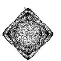
(a) limit

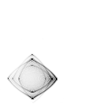
(b) probabilities at time 200

Figure 3: the $S(1/8)$ walk

Theorem 4.2.

For the quantum random walk with unitary matrix $U=S(t)$, let ${\cal G}^{\prime}$ be a compact subset of the interior of ${\cal G}$ such that the curvatures ${\cal K}({\bf z})$ at all points ${\bf z}\in{\bf W}(\hat{{\bf r}})$ are nonvanishing for all $\hat{{\bf r}}\in{\cal G}^{\prime}$. Fix chiralities $i,j$, let $G:=G^{(i,j)}$, and let $a_{\bf r}:=a_{r,s,n}$ denote the amplitude to be at position $(r,s)$ at time $n$. Then as $|{\bf r}|\to\infty$, uniformly over $\hat{{\bf r}}\in{\cal G}^{\prime}$,

$$a_{\bf r}=(-1)^{\delta}\frac{1}{2\pi|{\bf r}|}\sum_{{\bf z}\in{\bf W}}{\bf z}^{-{\bf r}}\frac{G({\bf z})}{|{\nabla_{\rm\log}}H({\bf z})|}\frac{1}{\sqrt{|{\cal K}({\bf z})|}}e^{-i\pi\tau({\bf z})/4}\,+O\left(|{\bf r}|^{-3/2}\right)$$ (4.12)

where $\delta=1$ if ${\nabla_{\rm\log}}H$ is a negative multiple of $\hat{{\bf r}}$ (so as to change the sign of the estimate) and zero otherwise. When $\hat{{\bf r}}\in[-1,1]^{2}\setminus{\cal G}$ then for every integer $N>0$ there is a $C>0$ such that $|a_{\bf r}|\leq C|{\bf r}|^{-N}$ with $C$ uniform as ${\bf r}$ ranges over a neighborhood ${\cal N}$ of ${\bf r}$ whose closure is disjoint from the closure of ${\cal G}$.

Before proving this theorem we interpret its implication for the probability profile. The probability of finding the particle at $(r,s)$ in the given chiralities at the given time is equal to $|a_{\bf r}|^{2}$. We only care about $a_{\bf r}$ up to a unit complex multiple, so we don’t care whether $\delta$ is zero or one, but we must keep track of phase factors inside the sum because these affect the interference of terms from different ${\bf z}\in{\bf W}$. In fact, the nearest neighbor QRW has periodicity (because all possible steps are odd); the manifestation of this is that ${\bf W}$ consists of conjugate pairs. When $r+s$ and $n$ have opposite parities the summands in the formula for $a_{\bf r}$ cancel. Otherwise the probability amplitude $|a_{\bf r}|^{2}$ will be $\Theta(n^{-2})$, uniformly over compact regions avoiding critical values in the range of the logarithmic Gauss map but blowing up at these values.

Proof of Theorem 4.2: As ${\cal G}\subset{\bf K}$ by lemma 4.1, the result when $\hat{{\bf r}}\in{\cal G}^{\prime}$ is immediate once we have shown that for any $S(t)$, its generating function satisfies the hypotheses of Theorem 3.3. We establish this in the lemma below.

Lemma 4.3.

Let $H:=H^{(p)}=\det\left(I-zM(x,y)S(t)\right)$. Then for $0<t<1$, $\nabla H\neq 0$ on $T_{3}$. Consequently, ${\cal V}_{1}:={\cal V}_{H}\ \cap T_{3}$ is smooth.

Theorem 3.3 will not be helpful in proving the case when $\hat{{\bf r}}\in[-1,1]^{2}\setminus{\cal G}$. To prove this condition we present the following lemma, which is a generalization of  [Ste, 93, Proposition 4 of Section VIII.2].

Lemma 4.4.

Let ${\cal M}$ be a compact $d$-manifold. Suppose $\alpha$ is smooth and that $f$ is a smooth function taking values in ${\mathbb{R}}/(2\pi L)$, with no critical points in ${\cal M}$. Then

$$I(\lambda)=\int_{{\cal M}}e^{i\lambda f(x)}\alpha(x)dx=O(\lambda^{-N})$$ (4.13)

as $\lambda\rightarrow\infty$ through multiples of $L$, for every $N\geq 0$.

We will see below that ${\cal V}_{1}$ is a fourfold (unbranched) cover of the two-torus. Any such cover is compact. In the calculation of $a_{{\bf r}}$, we have $f({\bf y})=-\hat{{\bf r}}\cdot{\bf y}$ and $\lambda=|{\bf r}|$. Thus a direction $\hat{{\bf r}}$ is not in ${\cal G}$ precisely when $f({\bf y})$ has no critical points in ${\cal V}_{1}$. Uniform exponential decay of amplitudes for ${\bf r}$ bounded outside the image of the Gauss map follows. $\hfill\Box$

We now prove the above lemmas in reverse order.

Proof of Lemma 4.4 : As ${\cal M}$ is compact it admits a finite open cover $\{U_{i}\}_{i\in I}$ with subordinate partition of unity $\{\phi_{i}\}_{i\in I}$. We decompose the integral

$$I(\lambda) = \int_{{\cal M}}e^{i\lambda f(x)}\alpha(x)dx$$

$$= \int_{{\cal M}}e^{i\lambda f(x)}\alpha(x)\sum_{i\in I}\phi_{i}(x)dx$$

$$= \sum_{i\in I}\int_{{\cal M}}e^{i\lambda f(x)}\alpha(x)\phi_{i}(x)dx$$

$$= \sum_{i\in I}\int_{U_{i}}e^{i\lambda f(x)}\alpha(x)\phi_{i}(x)dx$$

We will show that for each $i\in I$, $\int_{U_{i}}e^{i\lambda f(x)}\alpha(x)\phi_{i}(x)dx$ is rapidly decreasing (the requirement above for $I(\lambda)$). As the cover $U_{i}$ is finite, this will give us our result.

For a given $i\in I$, we let $\psi(x):=\alpha(x)\phi_{i}(x)$ which is then smooth with compact support. For each $x_{0}$ in the support of $\psi(x)$, there is a unit vector $\xi$ and a small ball $B(x_{0})$, centered at $x_{0}$, such that $\xi\cdot(\nabla f)(x)\geq c>0$ for some real $c$ uniformly for all $x\in B(x_{0})$. We then decompose the integral $\int_{U_{i}}e^{i\lambda f(x)}\psi(x)dx$ as a finite sum

$$\sum_{k}\int e^{i\lambda f(x)}\psi_{k}(x)dx\,$$

where each $\psi_{k}$ is smooth and has compact support in one of these balls. It then suffices to prove the corresponding estimate for each summand. Now choose a coordinate system $x_{1},\ldots,x_{d}$ so that $x_{1}$ lies along $\xi$. Then

$$\int e^{i\lambda f(x)}\psi_{k}(x)dx=\int\left(\int e^{i\lambda f(x_{1},\ldots,x_{d})}\psi_{k}(x_{1},...,x_{d})dx_{1}\right)dx_{2}\ldots dx_{d}$$

Now by [Ste, 93, Proposition 1 of Section VIII.2] the inner integral is rapidly decreasing, giving us our desired conclusion. $\hfill\Box$

For the next two proofs, we clear denominators to obtain the following explicit polynomial: $H=(x^{2}y^{2}+y^{2}-x^{2}-1+2xyz^{2})z^{2}-2xy-\sqrt{2t}z(xy^{2}-y-x+z^{2}y-z^{2}x+z^{2}xy^{2}+z^{2}x^{2}y-x^{2}y)$. We make the substitution $\alpha=\sqrt{2t}$ to facilitate the use of Gröbner Bases, which require polynomials as inputs. Use the notation $H_{x}$ for $\frac{\partial H}{\partial x}$, and similarly with $y$ and $z$.

Proof of Lemma 4.3:

Using the Maple command ${\tt Basis([H,H_{x},H_{y},H_{z}],plex(x,y,z,\alpha)}$ we get a Gröbner Basis with first term $z\alpha^{2}(\alpha^{2}-1)(\alpha^{2}-2)=2zt(2t-1)(2t-2)$. Thus to show that $S(t)$ results in a variety whose intersection with $T$ is smooth for $t\in(0,1)$, we need only consider the case when $t=1/2$. In this case $\alpha=1$ and the Gröbner Basis for the ideal where $(H,\nabla H)=\bf{0}$ is $(-z+z^{5},z^{3}+2y-z,-z-z^{3}+2x)$. Here $B_{1}$ vanishes on the unit circle for $z=\pm 1,\pm i$. However, for $z=\pm 1$, $B_{2}$ vanishes only when $y=0$ and for $z=\pm i$, $B_{3}$ vanishes only when $x=0$. Thus $\nabla H$ does not vanish on $T_{3}$. $\hfill\Box$

Further analysis of the limit shape for $S(t)$

Proposition 4.5.

For each pair $(x,y)$, there are four distinct values $z_{1},z_{2},z_{3},z_{4}$ such that $(x,y,z_{i})\in{\cal V}_{1}$ for $i\in{1,2,3,4}$. Consequently, the projection $(x,y,z)\mapsto(x,y)$ is a smooth four-covering of $T_{2}$ by ${\cal V}_{1}$.

Proof: Since $H$ has degree four in $z$, it has at most four $z$ values in ${\mathbb{C}}$ for each pair $(x,y)$, hence at most four $z$ values in ${\cal V}_{1}$. Recall from Proposition 2.1 that all solutions to $H(x,y,z)=0$ for a given $(x,y)$ in the unit torus have $|z|=1$ as well. Hence, if ever there are fewer than four $z$ values for a given $(x,y)$, then there are fewer than four solutions to $H(x,y,\cdot)=0$ and the implicit function theorem must fail. Consequently, $\frac{\partial H}{\partial z}=0$. This cannot be true, however, by the following argument. We have ruled out $H_{x}=H_{y}=H_{z}=0$ on ${\cal V}_{1}$, so if $H_{z}=0$, then the point $(x,y,z)$ contributes toward asymptotics in the direction $(r,s,0)$ for some $(r,s)\neq(0,0)$. The particle moves at most one step per unit time, so this is impossible. $\hfill\Box$

To facilitate discussions of subsets of the unit torus, we let $(\alpha,\beta,\gamma)$ denote the respective arguments of $(x,y,z)$, that is, $x=e^{i\alpha},y=e^{i\beta},z=e^{i\gamma}$. We may think of $\alpha,\beta$ and $\gamma$ as belonging to the flat torus $({\mathbb{R}}/2\pi{\mathbb{Z}})^{3}$.

Proposition 4.6.

${\cal V}_{1}$ can be decomposed into connected components as ${\cal V}_{1}=A\amalg B\amalg C\amalg D$, where $A,B,C$ and $D$ will be the components containing the $\gamma$ values $0,\pi/2,\pi$ and $3\pi/2$, respectively.

Proof: Let $\chi:=\{(x,y,z):z^{4}=-1\}$. We begin by establishing that $|{\cal V}_{1}\cap\chi|=8$ with two points for each of the fourth roots of $-1$. Furthermore, $-\pi/4\leq\gamma\leq\pi/4$ on $A$, $\pi/4\leq\gamma\leq 3\pi/4$ on $B$, $3\pi/4\leq\gamma\leq 5\pi/4$ on $C$, and $5\pi/4\leq\gamma\leq 7\pi/4$ on $D$. These observations suffice to prove the proposition, because the smooth variety ${\cal V}_{1}$ cannot have an intersection with a torus that is pinched down to a point; the only possibility is therefore that these values of $\gamma$ are extreme values on components of ${\cal V}_{1}$.

To check the first of these statements, use the identities $\cos\gamma=(z+z^{-1})/2$, $\sin\gamma=(z-z^{-1})/(2i)$, as well as the analogous identities for $\alpha$ and $\beta$, to write the equation of ${\cal V}$ in terms of $\alpha,\beta$ and $\gamma$. We find that $H(x,y,z)=0$ if and only if

$$0=L(\alpha,\beta,\gamma):=2\sin\gamma\cos\gamma-\sqrt{2t}(\sin\beta\cos\gamma+\cos\alpha\sin\gamma)+\cos\alpha\sin\beta\,.$$ (4.14)

Substituting $\gamma=\pi/4$ results in

$$1-(\sin\beta+\cos\alpha)\sqrt{t}+\cos\alpha\sin\beta=0\,.$$

Verifying that $\sin\beta=\sqrt{t}$ is not a solution, and dividing by $\sin\beta-\sqrt{t}$, we find that

$$\cos\alpha=\frac{1-\sqrt{t}\sin\beta}{\sin\beta-\sqrt{t}}\,.$$

The right-hand side is in $[-1,1]$ only when $\sin\beta=\pm 1$. Thus when $\gamma=\pi/4$, the pair $(\alpha,\beta)$ is either $(\pi,\pi/2)$ or $(0,3\pi/2)$.

To check the remaining statements, we introduce the following set of isometries for ${\cal V}_{1}$. Define

$$\phi_{A}(\alpha,\beta,\gamma) := \left(-\alpha,-\beta,-\gamma\right)$$

$$\phi_{B}(\alpha,\beta,\gamma) := \left(\beta+\frac{\pi}{2},\alpha+\frac{\pi}{2},\gamma+\frac{\pi}{2}\right)$$

$$\phi_{C}(\alpha,\beta,\gamma) := \left(\alpha+\pi,\beta+\pi,\gamma+\pi\right)$$

$$\phi_{D}(\alpha,\beta,\gamma) := \left(\beta+\frac{3\pi}{2},\alpha+\frac{3\pi}{2},\gamma+\frac{3\pi}{2}\right)$$

Verifying that $\phi_{A}$, $\phi_{B}$ and $\phi_{C}$ (and hence $\phi_{D}$ which is equal to $\phi_{C}\circ\phi_{B}$) are isometries is a simple exercise in trigonometry using equation 4.14, which we will omit. Each isometry inherits its name from the region it proves isometric with $A$. Using these isometries, we see that $\gamma$ is equal to $3\pi/4$, $5\pi/4$ and $7\pi/4$ exactly twice on ${\cal V}_{1}$. $\hfill\Box$

We remark upon the existence of an additional eight-fold isometry within each connected component: $\phi_{1}(\alpha,\beta,\gamma):=(\alpha,\beta+\pi,-\gamma)$, $\phi_{2}(\alpha,\beta,\gamma):=(-\alpha,\beta,\gamma)$ and $\phi_{3}(\alpha,\beta,\gamma):=(\alpha,\pi-\beta,\gamma)$. These symmetries manifest themselves in Figure 3 as follows. The image is clearly the superposition of two pieces, one horizontally oriented and one vertically oriented. Each of these two is the image of the Gauss map on two of the regions $A,B,C,D$, and each of these four regions maps to the plot in a 2 to 1 manner on the interior, folding over at the boundary. To verify this, we observe that if $p_{0}$ contributes to asymptotics in the direction $(r,s)$ then $\phi_{A}(p_{0}),\phi_{B}(p_{0}),\phi_{C}(p_{0}),\phi_{D}(p_{0}),\phi_{1}(p_{0}),\phi_{2}(p_{0})$ and $\phi_{3}(p_{0})$ contribute to asymptotics in the directions $(r,s)(s,r),(r,s),(s,r),(-r,-s),(-r,s)$ and $(r,-s)$, respectively. Thus while the image of the Gauss map is two overlapping leaves, the Gauss map of $A$ and $C$ contribute to one leaf, while the Gauss map of $B$ and $D$ contribute to the other.

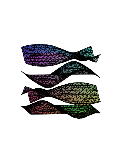
Figure 4: The variety ${\cal V}_{1}$ for $t=1/2$

We end the analysis with a few observations on the way in which the plots were generated. Our procedure was as follows. Solving for $\sin\gamma$ in (4.14), we obtained

$$\sin\gamma=\sin\beta\,\frac{\sqrt{2t}\;\cos\gamma-\cos\alpha}{2\cos\gamma-\sqrt{2t}\;\cos\alpha}\,.$$ (4.15)

Squaring (4.14) and making the substitution $\sin^{2}\gamma=1-\cos^{2}\gamma$, we found that

$$\left(1-\cos^{2}\gamma\right)\left(2\cos\gamma-\sqrt{2t}\;\cos\alpha\right)^{2}-\left(1-\cos^{2}\beta\right)\left(\sqrt{2t}\;\cos\gamma-\cos\alpha\right)^{2}=0\,$$

which we used to get the four solutions for $\gamma$ in terms of $\alpha$ and $\beta$. We then let $\alpha$ and $\beta$ vary over a grid embedded in the 2-torus and solved for the four values of $\gamma$ to obtain four points in ${\cal V}_{1}$; this is the composition of the first two maps in (1.2). Differentiation of $H(e^{i\alpha},e^{i\beta},e^{i\gamma})=0$ shows that the projective direction $(r,s,t)$ corresponding to a point $(\alpha,\beta,\gamma)$ is given by $r/t=-\partial\gamma/\partial\alpha,s/t=-\partial\gamma/\partial\beta$. Implicit differentiation of (4.14) then gives four explicit values for $(r/t,s/t)$ in terms of $\alpha$ and $\beta$. This is the composition of the last two maps in (1.2), with the parametrization of ${\mathbb{R}}{\mathbb{P}}^{2}$ by $(r/t,s/t)$ corresponding to the choice of a planar rather than a spherical slice.

4.2 The family $A(t)$

We now present a second family of orthogonal matrices $A(t)$ below. In order for the matrices to be real, we restrict $t$ to the interval $(0,1/\sqrt{3})$.

$$A(t)=\left(\begin{array}[]{cccc}t&t&t&\sqrt{1-3t^{2}}\\ -t&t&-\sqrt{1-3t^{2}}&t\\ t&-\sqrt{1-3t^{2}}&-t&t\\ -\sqrt{1-3t^{2}}&-t&t&t\end{array}\right)$$

This family intersects the family $S(t)$ in one case, namely $A(1/2)=S(1/2)$; for any $(t,t^{\prime})\in(0,1)^{2}$ other than $(1/2,1/2)$, we have $A(t)\neq S(t^{\prime})$. The following theorem follows from Lemma 4.4 along with a new lemma, namely Lemma 4.8 below, analogous to Lemma 4.3.

Theorem 4.7.

If $0<t<1/\sqrt{3}$ then Theorem 4.2 holds for the unitary matrix $A(t)$ in place of the matrix $S(t)$. $\hfill\Box$

Lemma 4.8.

Let $H:=H^{(t)}=\det\left(I-zM(x,y)A(t)\right)$. Then for $0<t<1/\sqrt{3}$, $\nabla H\neq 0$ on $T_{3}$. Consequently, ${\cal V}_{1}:={\cal V}_{H}\ \cap T_{3}$ is smooth.

Proof of Lemma 4.8: We clear our denominator by setting $H:=(-xy)\det(I-MA(t)z)$, now to get

$$H=2(x-1)(x+1)(y^{2}+1)z^{2}t^{2}-(-y-x+xy^{2}+z^{2}y-x^{2}y+z^{2}xy^{2}-z^{2}x+z^{2}x^{2}y)zt+(yz^{2}-x)(xz^{2}+y)\,.$$

As no $\sqrt{1-t^{2}}$ term appears, we can determine a Gröbner Basis without making a substitution. The Maple command ${\tt Basis([H,H_{x},H_{y},H_{z}],plex(x,y,z,t)}$ delivers a Basis with first term $t^{3}z(2t+1)(8t^{2}-3)(2t^{2}-1)(2t-1)$. The roots of the first four factors fall outside of our interval $(0,1/\sqrt{3})$ while the root of the last factor corresponds to the matrix $S(1/2)$ for which we know ${\cal V}_{1}$ is smooth from the discussion above. $\hfill\Box$

Again we use theorem 3.3 to correctly predict asymptotics for individual directions. We show probability profiles for a number of parameter values.

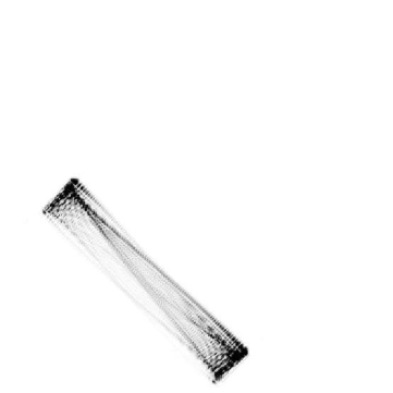
Figure 5: The profile for $A(1/6)$ shows how the QRW approaches degeneracy at the endpoints $t\to 0,1$

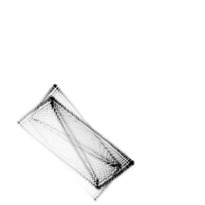
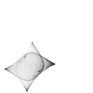
Figure 6: $t$ increases from $1/3$ to $5/9$, switching the direction of the tilt

4.3 The family $B(t)$

To demonstrate the application of theorem 3.5 we introduce a third family of orthogonal matrices, $B(t)$, with $t\in(0,1)$.

$$B(t)=\left(\begin{array}[]{cccc}\frac{\sqrt{t}}{\sqrt{2}}&\frac{\sqrt{t}}{\sqrt{2}}&\frac{\sqrt{1-t}}{\sqrt{2}}&\frac{\sqrt{1-t}}{\sqrt{2}}\\ -\frac{\sqrt{t}}{\sqrt{2}}&\frac{\sqrt{t}}{\sqrt{2}}&-\frac{\sqrt{1-t}}{\sqrt{2}}&\frac{\sqrt{1-t}}{\sqrt{2}}\\ -\frac{\sqrt{1-t}}{\sqrt{2}}&\frac{\sqrt{1-t}}{\sqrt{2}}&\frac{\sqrt{t}}{\sqrt{2}}&-\frac{\sqrt{t}}{\sqrt{2}}\\ -\frac{\sqrt{1-t}}{\sqrt{2}}&-\frac{\sqrt{1-t}}{\sqrt{2}}&\frac{\sqrt{t}}{\sqrt{2}}&\frac{\sqrt{t}}{\sqrt{2}}\end{array}\right)$$

We have already seen a walk generated by such a matrix, as Figure 1 depicted the walk generated by $B(1/2)$. We note that $B(t)$ is almost identical to $S(t)$ with the one exception being the multiplication of the third row by $-1$. As was the case with the $S(t)$ walks we can see strong similarities between the image of the Gauss map and the probability profile for various values of $t$.

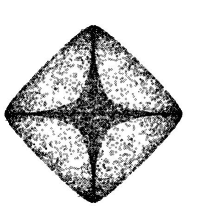
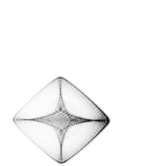
Figure 7: The image of the Gauss map alongside the probability profile for the $B(2/3)$ walk

In contrast to the cases of $S(t)$ and $A(t)$, we will not be able to apply Theorem 3.3 because ${\cal V}_{1}$ is not smooth.

Theorem 4.9.

For the quantum random walk with unitary matrix $U=B(t)$, let ${\cal G}^{\prime}$ be a compact subset of the interior of ${\cal G}$ such that the curvatures ${\cal K}({\bf z})$ at all points ${\bf z}\in{\bf W}(\hat{{\bf r}})$ are nonvanishing for all $\hat{{\bf r}}\in{\cal G}^{\prime}$. Then as $|{\bf r}|\to\infty$, uniformly over $\hat{{\bf r}}\in{\cal G}^{\prime}$,

$$a_{\bf r}=\pm\frac{1}{2\pi|{\bf r}|}\sum_{{\bf z}\in{\bf W}}{\bf z}^{-{\bf r}}\frac{G({\bf z})}{|{\nabla_{\rm\log}}H({\bf z})|}\frac{1}{\sqrt{|{\cal K}({\bf z})|}}e^{-i\pi\tau({\bf z})/4}\,+O\left(|{\bf r}|^{-3/2}\right)\,.$$ (4.16)

When $\hat{{\bf r}}\in[-1,1]^{2}\setminus{\cal G}$ then for every integer $N>0$ there is a $C>0$ such that $|a_{\bf r}|\leq C|{\bf r}|^{-N}$ with $C$ uniform as ${\bf r}$ ranges over a neighborhood ${\cal N}$ of ${\bf r}$ whose closure is disjoint from the closure of ${\cal G}$.

Proof: First, we apply lemma 4.4 with the lemma being applicable as we will see below that ${\cal V}_{1}:={\cal V}_{H}\cap T_{3}$ is a two-fold cover of $T_{2}$ and thus compact. The conclusion when $\hat{{\bf r}}\in[-1,1]^{2}\setminus{\cal G}$ follows. We get the conclusion in the case where $\hat{{\bf r}}\in{\cal G}^{\prime}$ by verifying the hypotheses of theorem 3.5 in the following lemmas.

Lemma 4.10.

Let $H:=H^{(t)}=\det\left(I-zM(x,y)B(t)\right)$. Then for $0<t<1$, the set ${\cal W}=\{(x,y,z):(H,\nabla H)=0\}$ consists only of the four points $(x,y,z)=\pm(1,1,\sqrt{t/2}\pm i\sqrt{1-t/2})$.

Lemma 4.11.

For any $0<t<1$ we have the following conclusions for each $p_{0}\in{\cal W}$ for the generating function associated to the unitary matrix $U=B(t)$.

1. The residue form $\eta$ has leading degree $\alpha>d/2$ at $p_{0}$.

2. The cone ${\cal V}_{p_{0}}$ is projectively smooth and ${\bf r}$ is not in the normal cone to ${\cal V}$ at $p_{0}$.

Proof of Lemma 4.10: The proof of Lemma 4.10 is similar to the corresponding proofs in the two previous examples, so we give only a sketch. Computing $H$ from (2.3) and the subsequent formula yields

$$H = 2xy(z^{4}+1)-(x+y+xy^{2}+x^{2}y)(z^{3}+z)\sqrt{2t}+(4txy+x^{2}+x^{2}y^{2}+1+y^{2})z^{2}$$

$$= xyz^{2}\cdot\left[4t+\right.$$

$$\left.2(z^{2}+z^{-2})-\left((x+x^{-1})+(y+y^{-1})\right)(z+z^{-1})\sqrt{2t}+(x+x^{-1})(y+y^{-1})\right]\,,$$

Treating $t$ as a parameter and computing a Gröbner basis of $\{H,H_{x},H_{y},H_{z}\}$ with term order $\mbox{ \tt plex}(x,y,z)$ one obtains $\{x^{3}-x,y-x,z(x^{2}-1),z^{2}-2x\sqrt{t}z+2x^{2}\}$. Removing the extraneous roots when one of $x,y$ or $z$ vanishes, what remains is $\pm(1,1,z)$ where $z$ solves $z^{2}-2\sqrt{t}z+2=0$. $\hfill\Box$

Proof of Lemma 4.11: Condition $(i)$ follows from the fact that for each $p_{0}\in{\cal W}$, the numerator $G^{(p)}(x,y,z)$ vanishes as well as the denominator $H^{(p)}$ which only vanishes to order 1. To prove $(ii)$, we compute the local geometry of $\{H=0\}$ near the four points found in the previous lemma. We will do this for the points with positive $(x,y)=(1,1)$; the case $(x,y)=(-1,-1)$ is similar. Substituting $x=1+u,y=1+v,z=z_{0}+w$ into $H$ and then reducing modulo $z_{0}^{2}-2\sqrt{t}z_{0}+2$, we find that the leading homogeneous term in the variables $\{u,v,w\}$ is $4[\sqrt{t}(1-t)(u^{2}+v^{2})-(2-t)w^{2}]$. For $0<t<1$, this is the cone over a nondegenerate ellipse and therefore smooth. The dual cone is the set of $(r,s,u)$ with $r^{2}+s^{2}=\frac{2-t}{(1-t)\sqrt{t}}u^{2}$. The minimum value of $\frac{2-t}{(1-t)\sqrt{t}}$ on $[0,1]$ is greater than 4, while the vectors $(r,s,u)$ inside the image of the Gauss map all have $r^{2}+s^{2}<4u^{2}$, whence ${\bf r}$ is never in the normal cone to ${\cal V}$ at $p_{0}$. $\Box$

Beginning with (4.3), we see that $(x,y,z)\in{\cal V}_{1}\iff$

$$2\cos^{2}\gamma-\left(\cos\alpha+\cos\beta\right)\sqrt{2t}\cos\gamma+\cos\alpha\cos\beta+t-1=0\,.$$ (4.18)

Thus for given $\alpha$ and $\beta$, the four values of $\gamma$ are given explicitly by

$$\gamma=\pm\arccos\left[\frac{\left(\cos\alpha+\cos\beta\right)\sqrt{2t}\pm\sqrt{2t\left(\cos\alpha+\cos\beta\right)^{2}-8\cos\alpha\cos\beta-8t+8}}{4}\right]\,.$$ (4.19)

We then differentiate  4.18 with respect to $\alpha$ and $\beta$ to obtain the partial derivatives

$$\frac{\partial\gamma}{\partial\alpha}=\frac{\sin\alpha}{\sin\gamma}\cdot\frac{\cos\beta-\sqrt{2t}\cos\gamma}{\sqrt{2t}(\cos\alpha+\cos\beta)-4\cos\gamma}$$

and

$$\frac{\partial\gamma}{\partial\beta}=\frac{\sin\beta}{\sin\gamma}\cdot\frac{\cos\alpha-\sqrt{2t}\cos\gamma}{\sqrt{2t}(\cos\alpha+\cos\beta)-4\cos\gamma}\,.$$

Remark.

The fact that we can solve explicitly for $\gamma$ with this family allows us to more clearly depict the connection between curvature and asymptotics. Using Proposition 2.3 and (4.19), we let Maple evaluate $\nabla$ as well as

${\cal H}=\left[\begin{array}[]{cc}\frac{\partial^{2}\gamma}{\partial\alpha^{2}}&\frac{\partial^{2}\gamma}{\partial\alpha\partial\beta}\\ \frac{\partial^{2}\gamma}{\partial\beta\partial\alpha}&\frac{\partial^{2}\gamma}{\partial\alpha^{2}}\end{array}\right]$

We then plot ${\cal K}$ against $-\frac{\partial\gamma}{\partial\alpha}$ and $-\frac{\partial\gamma}{\partial\beta}$ as $(\alpha,\beta)$ varies over the two-dimensional torus.

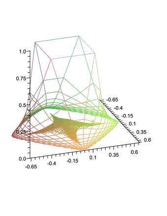
Figure 8: A graph of curvature versus direction for the $B(1/2)$ walk

In the above picture we see the expected cross within a diamond region where curvature is low, though the view is obstructed by regions of higher curvature.

To remedy this problem we restrict our view of the ${\cal K}$ axis to focus on the smallest values of ${\cal K}$ which in turn contribute to the largest probabilities. The resulting picture thus predicts the regions that will appear darkest in the probability profile.

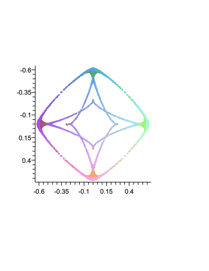
Figure 9: A graph of the areas of lowest curvature and hence highest probabilities for the $B(1/2)$ walk

References

- ABG [70] M. Atiyah, R. Bott, and L. Gårding. Lacunas for hyperbolic differential operators with constant coefficients, I. Acta Mathematica, 124:109–189, 1970.
- ABN+ [01] A. Ambainis, E. Bach, A. Nayak, A. Vishwanath, and J. Watrous. One-dimensional quantum walks. In Proceedings of the 33rd Annual ACM Symposium on Theory of Computing, pages 37–49, New York, 2001. ACM Press.
- ADZ [93] Y. Aharonov, L. Davidovich, and N. Zagury. Quantum random walks. Phys. Rev. A, 48:1687–1690, 1993.
- BH [86] N. Bleistein and R. A. Handelsman. Asymptotic Expansions of Integrals. Dover Publications Inc., New York, second edition, 1986.
- BK [86] E. Brieskorn and H. Knörrer. Plane algebraic curves. Birkhäuser, Basel, 1986.
- BP [07] A. Bressler and R. Pemantle. Quantum random walks in one dimension via generating functions. In Proceedings of the 2007 Conference on the Analysis of Algorithms, volume AofA 07, page 11. LORIA, Nancy, France, 2007.
- BP [08] Y. Baryshnikov and R. Pemantle. Tilings, groves and multiset permutations: asymptotics of rational generating functions whose pole set is a cone. arXiv, http://front.math.ucdavis.edu/0810.4898: 79, 2008.
- Bra [07] W. Brady. Quantum random walks on . Master of Philosophy Thesis, The University of Pennsylvania, 2007.
- CIR [03] Hilary A. Carteret, Mourad E. H. Ismail, and Bruce Richmond. Three routes to the exact asymptotics for the one-dimensional quantum walk. J. Phys. A, 36:8775–8795, 2003.
- GJ [83] I. P. Goulden and D. M. Jackson. Combinatorial enumeration. A Wiley-Interscience Publication. John Wiley & Sons Inc., New York, 1983. With a foreword by Gian-Carlo Rota, Wiley-Interscience Series in Discrete Mathematics.
- GKZ [94] I. Gelfand, M. Kapranov, and A. Zelevinsky. Discriminants, Resultants and Multidimensional Determinants. Birkhäuser, Boston-Basel-Berlin, 1994.
- GP [74] V. Guillemin and A. Pollack. Differential Topology. Prentice-Hall, Inc., Englewood Cliffs, NJ, 1974.
- Gro [96] L. Grover. A fast quantum mechanical algorithm for database search. Annual ACM Symposium on Theory of Computing, pages 212–219, 1996. Proceedings of the twenty-eighth annual ACM symposium on Theory of computing.
- IKK [04] N. Innui, Y. Konishi, and N. Konno. Localization of two-dimensional quantum walks. Physical Review A, 69:052323–1 – 052323–9, 2004.
- IKS [05] N. Inui, N. Konno, and E. Segawa. One-dimensional three-state quantum walk. Phys. Rev. E, 72:7, 2005.
- MBSS [02] T. Mackay, S. Bartlett, L. Stephanson, and B. Sanders. Quantum walks in higher dimensions. Journal of Physics A, 35:2745–2754, 2002.
- PW [02] R. Pemantle and M.C. Wilson. Asymptotics of multivariate sequences. I. Smooth points of the singular variety. J. Combin. Theory Ser. A, 97(1):129–161, 2002.
- PW [04] R. Pemantle and M.C. Wilson. Asymptotics of multivariate sequences, II. Multiple points of the singular variety. Combin. Probab. Comput., 13:735–761, 2004.
- PW [08] R. Pemantle and M.C. Wilson. Twenty combinatorial examples of asymptotics derived from multivariate generating functions. SIAM Review, 50:199–272, 2008.
- Sta [97] R. P. Stanley. Enumerative Combinatorics. Vol. 1. Cambridge University Press, Cambridge, 1997. With a foreword by Gian-Carlo Rota, Corrected reprint of the 1986 original.
- Ste [93] E. Stein. Harmonic Analysis: Real-Variable Methods, Orthogonality, and Oscillatory Integrals. Princeton University Press, Princeton, NJ, 1993. With the assistance of Timothy S. Murphy, Monographs in Harmonic Analysis, III.
- Tou [68] J.C. Tougeron. Idéaux et fonctions differéntiables. i. Annales de l’Institut Fourier, 18:177–240, 1968.
- WKKK [08] K. Watabe, N. Kobayashi, M. Katori, and N. Konno. Limit distributions of two-dimensional quantum walks. Physical Review A, 77:062331–1 – 062331–9, 2008.
- Won [89] R. Wong. Asymptotic Approximations of Integrals. Academic Press Inc., Boston, MA, 1989.