Three-dimensional discrete systems of Hirota-Kimura type and deformed Lie-Poisson algebras

Abstract.

Recently Hirota and Kimura presented a new discretization of the Euler top with several remarkable properties. In particular this discretization shares with the original continuous system the feature that it is an algebraically completely integrable bi-Hamiltonian system in three dimensions. The Hirota-Kimura discretization scheme turns out to be equivalent to an approach to numerical integration of quadratic vector fields that was introduced by Kahan, who applied it to the two-dimensional Lotka-Volterra system.

The Euler top is naturally written in terms of the $\mathfrak{so}(3)$ Lie-Poisson algebra. Here we consider algebraically integrable systems that are associated with pairs of Lie-Poisson algebras in three dimensions, as presented by Gümral and Nutku, and construct birational maps that discretize them according to the scheme of Kahan and Hirota-Kimura. We show that the maps thus obtained are also bi-Hamiltonian, with pairs of compatible Poisson brackets that are one-parameter deformations of the original Lie-Poisson algebras, and hence they are completely integrable. For comparison, we also present analogous discretizations for three bi-Hamiltonian systems that have a transcendental invariant, and finally we analyze all of the maps obtained from the viewpoint of Halburd’s Diophantine integrability criterion.

^†Institute of Mathematics, Statistics and Actuarial Science,

University of Kent,

Canterbury CT2 7NF, UK

e-mail: A.N.W.Hone@kent.ac.uk

^♭Dipartimento di Fisica,

Università degli Studi Roma Tre and Sezione INFN, Roma Tre,

Via della Vasca Navale 84, 00146 Roma, Italy

e-mail: petrera@fis.uniroma3.it

1. Introduction

The problem of numerical integration, namely that of approximating the flow of a smooth vector field by an iterative scheme given in terms of a difference equation or a map, is one of the central problems of numerical analysis. If the underlying differential equation is Hamiltonian, or volume-preserving, or has some other important geometrical feature (such as being invariant under the action of a Lie group of symmetries), then as far as possible one would like to select a discretization scheme which preserves this feature, and this has led to the development of geometrical integration methods [4]. For the special case of completely integrable systems, ideally one would like to obtain discretizations which are themselves completely integrable. The area of integrable discretization has been developed quite extensively, especially from the Hamiltonian viewpoint, and a comprehensive review of the field can be found in the monograph [39]. In this paper we are concerned with a novel approach to discretization, which was used by Hirota and Kimura to obtain new integrable discrete analogues of the Euler and Lagrange tops [15, 22].

The discretization method studied in this paper seems to be introduced in the geometric integration literature by W. Kahan in the unpublished notes [20]. It is applicable to any system of ordinary differential equations for ${\bf x}:\mathbb{R}\to\mathbb{R}^{n}$ with a quadratic vector field

$$\dot{{\bf x}}=Q({\bf x})+B{\bf x}+{\bf c},$$

where each component of $Q:\mathbb{R}^{n}\to\mathbb{R}^{n}$ is a quadratic form, while $B\in{\rm Mat}_{n\times n}(\mathbb{R})$ and ${\bf c}\in\mathbb{R}^{n}$. Kahan’s discretization reads as

$$\frac{\widetilde{{\bf x}}-{\bf x}}{2\epsilon}=Q({\bf x},\widetilde{{\bf x}})+\frac{1}{2}B({\bf x}+\widetilde{{\bf x}})+{\bf c},$$ (1)

where

$$Q({\bf x},\widetilde{{\bf x}})=\frac{1}{2}\left[Q({\bf x}+\widetilde{{\bf x}})-Q({\bf x})-Q(\widetilde{{\bf x}})\right],$$

is the symmetric bilinear form corresponding to the quadratic form $Q$. Here and below we use the following notational convention which will allow us to omit a lot of indices: for a sequence ${\bf x}:\mathbb{Z}\to\mathbb{R}$ we write ${\bf x}$ for ${\bf x}_{k}$ and $\widetilde{{\bf x}}$ for ${\bf x}_{k+1}$. Eq. (1) is linear with respect to $\widetilde{\bf x}$ and therefore defines a rational map $\widetilde{{\bf x}}=f({\bf x},\epsilon)$. Clearly, this map approximates the time-$(2\epsilon)$-shift along the solutions of the original differential system, so that ${\bf x}_{k}\approx{\bf x}(2k\epsilon)$. (We have chosen a slightly unusual notation $2\epsilon$ for the time step, in order to avoid appearance of powers of 2 in numerous formulae; a more standard choice would lead to changing $\epsilon\mapsto\epsilon/2$ everywhere.) Since Eq. (1) remains invariant under the interchange ${\bf x}\leftrightarrow\widetilde{{\bf x}}$ with the simultaneous sign inversion $\epsilon\mapsto-\epsilon$, one has the reversibility property $f^{-1}({\bf x},\epsilon)=f({\bf x},-\epsilon).$ In particular, the map $f$ is birational.

Kahan applied this discretization scheme to the famous Lotka-Volterra system and showed that in this case it possesses a very remarkable non-spiralling property. Some further applications of this discretization have been explored in [21, 36].

The next, even more intriguing, appearance of this discretization was in the two papers by R. Hirota and K. Kimura who (being apparently unaware of the work by Kahan) applied it to two famous integrable systems of classical mechanics, the Euler top and the Lagrange top [15, 22]. Surprisingly, the Kahan-Hirota-Kimura discretization scheme produced integrable maps in both the Euler and the Lagrange cases of rigid body motion. Even more surprisingly, the mechanism which assures integrability in these two cases seems to be rather different from the majority of examples known in the area of integrable discretizations, and, more generally, integrable maps, cf. [39]. We shall use the term “Hirota-Kimura type discretization” for Kahan’s discretization in the context of integrable systems.

In the recent paper [32] the Hirota-Kimura integrability mechanism has been further investigated and its application to the integrable (six-dimensional) Clebsch system has been considered. The integrability of the Hirota-Kimura type discretization of the Clebsch system has been established, in the sense of: i) existence, for every initial point, of a four-dimensional pencil of quadrics containing the orbit of this point; ii) existence of four functionally independent integrals of motion. Note that for the purposes of paper [32], integrability of a dynamical system is synonymous with the existence of a sufficient number of functionally independent conserved quantities, or integrals of motion, that is, functions constant along the orbits. Other aspects of the notion of integrability, such as Hamiltonian properties or explicit solutions, still require further investigation. However, it is known that algebraically completely integrable cases of geodesic flow on $SO(4)$ are related to the intersection of four quadrics in $\mathbb{P}^{6}$ [2]. The Hirota-Kimura method of discretization has been recently applied to the classical three-dimensional nonholonomic Suslov problem in [7].

The above examples of Hirota-Kimura type discretizations suggested the following

Conjecture [32]. For any algebraically completely integrable system with a quadratic vector field, its Hirota-Kimura type discretization is algebraically completely integrable.

Since algebraically completely integrable systems generically correspond to linear flows on abelian varieties [40], this statement should be related to addition theorems for multi-dimensional theta-functions.

The aim of this paper is both to study how this novel method of discretization applies to a set of algebraically integrable systems in three dimensions, and to see how these results compare with the analogous discretizations of some quadratic vector fields with transcendental invariants. The former set of systems considered are algebraically integrable in the sense that they have a sufficient number of algebraic integrals in involution; however, there are various other (more stringent) notions of algebraic complete integrability. Through this study we are able both to verify the above conjecture for a new set of examples, and to gain further understanding of how the integrability of the discretization depends on the algebraic nature (or otherwise) of the integrals of motion in the original continuous system. Kahan’s discrete Lotka-Volterra system illustrates the subtlety of this dependence, as we now describe.

Kahan used his approach to discretize the Lotka-Volterra system

$$\dot{x}=x(1-y),\qquad\dot{y}=y(x-1),$$

which preserves the Poisson bracket $\{x,y\}=xy$, or equivalently, the symplectic form $1/(xy)\,dx\wedge dy$. This is an integrable system with one degree of freedom, $\dot{x}=\{x,H\}$, $\dot{y}=\{y,H\}$ with Hamiltonian

$$H=\log xy-(x+y).$$

Kahan’s discretization for this system reads [20]

$$\frac{\widetilde{x}-x}{\epsilon}=\widetilde{x}+x-\widetilde{x}y-x\widetilde{y},\qquad\frac{\widetilde{y}-y}{\epsilon}=-\widetilde{y}-y+\widetilde{x}y+x\widetilde{y}.$$ (2)

This discretization preserves the same symplectic structure as the original system of ordinary differential equations, for which it provides a numerically stable integration scheme which appears to retain the qualitative features of the continuous orbits (which are closed curves $H=\,$constant in the positive quadrant $x>0$, $y>0$) [37].

In fact, as noted in [31], Kahan’s discrete Lotka-Volterra system is algebraically integrable for $\epsilon=\pm 1$. To be precise, when $\epsilon=1$, it reduces to the second order recurrence $x_{n+1}x_{n-1}=x_{n}(2-x_{n})$ for the $x$ coordinate, which belongs to the class of antisymmetric QRT maps studied in [43]. This recurrence is linearizable (the iterates satisfy a linear recurrence of sixth order [19]), and the map has the integral

$$\widehat{H}=\frac{x^{2}}{y^{2}}+\frac{y^{2}}{x^{2}}+4\left(\frac{1}{x}-\frac{1}{y}\right)^{2}(1-x-y),$$

which (for fixed $\widehat{H}$) defines a quartic curve of genus zero; this is also an integral for $\epsilon=-1$ (which can be seen immediately from the reversibility property of Kahan’s discretization scheme). However, for other non-zero values of $\epsilon$, Kahan’s discrete Lotka-Volterra system should not be algebraically integrable; we present some numerical evidence for this in section 7 below. Indeed, since the integral $H$ for the original system is transcendental, from continuity arguments one would expect that (at least for small enough $\epsilon$) any integral of the the discretization should be transcendental as well. Further numerical studies, as mentioned in [32], indicate that this discrete system may well be non-integrable, with characteristics of chaos only evident by zooming in deeply on regions of the phase plane.

The outline of the paper is as follows. In the next section, we briefly review the Euler top together with the discrete Euler top found by Hirota and Kimura. In section 3 we describe six quadratic bi-Hamiltonian flows in three dimensions, which were presented in [11] (extending results in [3]), and are associated with pairs of real three-dimensional Lie algebras. Moreover, each of these systems, which we denote by ${\mathcal{E}}_{i}$ for $i=1,\ldots,6$, is algebraically integrable; the system ${\mathcal{E}}_{6}$ is equivalent to a special case of the Euler top. The fourth section is devoted to applying the Hirota-Kimura discretization scheme to these six systems, to obtain discrete systems (or maps) in three dimensions which we denote by $d{\mathcal{E}}_{i}$, and in section 5 we present the explicit solutions of these maps for $i=1,\ldots,5$ (the case $i=6$ being already included in the work of Hirota and Kimura [15]). Section 6 is concerned with applying the same discretization method to three other bi-Hamiltonian systems from [11] which have transcendental integrals. In section 7 we present the results of applying Halburd’s Diophantine integrability test to each of the maps obtained, and prove that all but one of them are Diophantine integrable in the sense of [12]. The final section is devoted to some conclusions.

2. Euler top and its Hirota-Kimura type discretization

The $\mathfrak{so}(3)$ Euler top is a well-known three-dimensional bi-Hamiltonian system belonging to the realm of classical mechanics [34]. The differential equations of motion of the Euler top read

$$\dot{x}=\alpha_{1}yz,\qquad\dot{y}=\alpha_{2}zx,\qquad\dot{z}=\alpha_{3}xy,$$ (3)

with $\alpha_{i}$ being real parameters of the system. We recall that this system can be explicitly integrated in terms of elliptic functions, and admits two functionally independent integrals of motion. Indeed, a quadratic function $H({\bf x})=\gamma_{1}x^{2}+\gamma_{2}y^{2}+\gamma_{3}z^{2}$ is an integral for Eqs. (3), if $\gamma_{1}\alpha_{1}+\gamma_{2}\alpha_{2}+\gamma_{2}\alpha_{2}=0$. In particular, the following three functions are integrals of motion:

$$H_{1}=\alpha_{3}y^{2}-\alpha_{2}z^{2},\qquad H_{2}=\alpha_{1}z^{2}-\alpha_{3}x^{2},\qquad H_{3}=\alpha_{2}x^{2}-\alpha_{1}y^{2}.$$

Clearly, only two of them are functionally independent because of $\alpha_{1}H_{1}+\alpha_{2}H_{2}+\alpha_{3}H_{3}=0$.

The Hirota-Kimura discretization of the Euler top introduced in [15] reads as

$$\left\{\begin{array}[]{l}\widetilde{x}-x=\epsilon\alpha_{1}(\widetilde{y}z+y\widetilde{z}),\\ \widetilde{y}-y=\epsilon\alpha_{2}(\widetilde{z}x+z\widetilde{x}),\\ \widetilde{z}-z=\epsilon\alpha_{3}(\widetilde{x}y+x\widetilde{y}).\end{array}\right.$$ (4)

Thus, the map $f:{\bf x}\mapsto\widetilde{\bf x}$ obtained by solving (4) for $\widetilde{{\bf x}}$, is given by:

$$\widetilde{{\bf x}}=f({\bf x},\epsilon)=A^{-1}({\bf x},\epsilon){\bf x},\qquad A({\bf x},\epsilon)=\begin{pmatrix}1&-\epsilon\alpha_{1}z&-\epsilon\alpha_{1}y\\ -\epsilon\alpha_{2}z&1&-\epsilon\alpha_{2}x\\ -\epsilon\alpha_{3}y&-\epsilon\alpha_{3}x&1\end{pmatrix}.$$ (5)

Apart from the Lax representation which is still unknown, the discretization (5) exhibits all the usual features of an integrable map: an invariant volume form, a bi-Hamiltonian structure (that is, two compatible invariant Poisson structures), two functionally independent conserved quantities in involution, and solutions in terms of elliptic functions. For further details about the properties of this discretization we refer to [15] and [30].

3. Some bi-Hamiltonian flows related to real three-dimensional Lie algebras

Hamiltonian systems in three dimensions provide the simplest non-trivial examples of degenerate Poisson structures, where the rank of the Poisson tensor is less than the dimension of the phase space. In three dimensions, a non-trivial Poisson tensor $P$ has rank two at generic points of the phase space, which means that (at least locally) there exists a Casimir function $K$ and another function $\phi$ such that

$$\{x_{j},x_{k}\}=\varepsilon_{jkl}\,\phi\,\frac{\partial K}{\partial x_{l}}$$ (6)

in local coordinates $x_{1},x_{2},x_{3}$; cf. Theorem 5 in [9]. This can be expressed in invariant form, by using the standard volume three-form $\Omega=dx_{1}\wedge dx_{2}\wedge dx_{3}$ in $\mathbb{R}^{3}$ to associate $P$ with the one-form $J=P\lrcorner\,\Omega=\phi\,dK$. An important thing to observe from the form of the Poisson bracket (6) is that in three dimensions the Poisson tensor can be multiplied by an arbitrary function while preserving the Jacobi identity.

Given an Hamiltonian system

$$\dot{\bf x}=\{{\bf x},H\}$$

defined in terms of the bracket (6) with an Hamiltonian function $H$ (functionally independent of $K$), it is clear that the equations of motion have two independent integrals, namely $H$ and $K$. Moreover, by fixing the value of the Casimir function (which may not be defined everywhere), we can regard this locally as a system with one degree of freedom which is integrable on each of the two-dimensional symplectic leaves $K=\mathrm{constant}$. However, for complete integrability the global existence of $H$ and $K$ is required.

Gümral and Nutku made a detailed study of the geometry of three-dimensional Poisson structures, and considered the conditions for the existence of globally integrable bi-Hamiltonian structures [11]. For a given three-dimensional system to be bi-Hamiltonian it is necessary and sufficient that the Jacobian at an arbitrary point be a Poisson tensor and that there exist two globally defined and (almost everywhere) functionally independent integrals of motion. Associated with two independent integrals $K$ and $H$, there are two compatible Poisson tensors, such that $K$ is the Casimir for one Poisson structure while $H$ is the Casimir for the other. In other words, if the dimension is three then two compatible Poisson tensors are completely determined by the constants of motion, and according to a relevant Theorem by Magri [24], provided certain technical conditions are satisfied, bi-Hamiltonian systems are completely integrable in the sense of Liouville-Arnold. Furthermore, in this setting there is an invariant volume form $\Omega$ (not necessarily canonical) which is preserved by the bi-Hamiltonian flow. An important example of such flows corresponds to Nambu mechanics [28], given by

$$\dot{\bf x}=\nabla H\times\nabla K,$$

which in these coordinates gives a divergenceless vector field ($\mathrm{div}\,\dot{\bf x}=0$); this means that the canonical measure is preserved by the flow. In particular, the Euler top is an example of Nambu mechanics in three dimensions; for other examples of Nambu mechanics in optics and elsewhere, see [17].

In [11] the authors present a list of all non-trivial bi-Hamiltonian flows that are associated with pairs of real three-dimensional Lie algebras and their Casimir invariants (as described in [29]); this list extends results in [3]. To be more precise, they consider pairs of real Lie-Poisson algebras defined by pairs of linear Poisson structures $P,Q$, and write down vector fields $\dot{\bf x}={\ V}$ satisfying

$${\ V}=-P\,dK=-\frac{1}{c}\,Q\,dH,$$

where $K$ is the Casimir for $Q$, while $H$ is the Casimir for $P$ (and minus signs are included in order to be consistent with the conventions of Gümral and Nutku). In [11] twelve such systems are presented, extending a list in [3], and each flow preserves a corresponding measure given in coordinates $(x_{1},x_{2},x_{3})=(x,y,z)$ by

$$\Omega=c\,dx\wedge dy\wedge dz,$$

related to the standard volume form by the conformal factor (or multiplier) $c$.

To begin with, we shall be concerned with only six out of the twelve systems in Gümral and Nutku’s list, namely the ones which have non-transcendental integrals of motion. They read

$${\mathcal{E}}_{1}:\qquad\dot{x}=-x^{2},\;\;\,\;\;\;\;\,\;\;\;\;\;\;\;\qquad\dot{y}=-xy,\qquad\qquad\;\;\dot{z}=2y^{2}+xz\,;$$ (7)

$${\mathcal{E}}_{2}:\qquad\dot{x}=-x^{2},\;\;\,\;\;\;\;\,\;\;\;\;\;\;\;\qquad\dot{y}=xy,\qquad\qquad\;\;\;\;\;\dot{z}=-2y^{2}+xz\,;$$ (8)

$${\mathcal{E}}_{3}:\qquad\dot{x}=-xz,\qquad\qquad\!\qquad\dot{y}=-yz,\qquad\qquad\,\;\;\dot{z}=x^{2}+y^{2}\,;$$ (9)

$${\mathcal{E}}_{4}:\qquad\dot{x}=-xz,\qquad\qquad\!\qquad\dot{y}=yz,\qquad\qquad\;\;\;\,\;\;\dot{z}=x^{2}-y^{2}\,;$$ (10)

$${\mathcal{E}}_{5}:\qquad\dot{x}=xy,\;\;\;\;\;\,\;\;\qquad\;\;\qquad\dot{y}=-x^{2},\qquad\;\,\;\,\,\;\;\;\;\;\;\dot{z}=y(2x-z)\,;$$ (11)

$${\mathcal{E}}_{6}:\qquad\dot{x}=y(2z-x),\qquad\;\;\;\;\;\;\dot{y}=x^{2}-z^{2},\qquad\;\;\;\;\;\dot{z}=y(z-2x)\,.$$ (12)

These six systems are examples of algebraically completely integrable systems, in the sense that in each case the integrals are algebraic (in fact, rational) functions of the coordinates $x,y,z$ for which the Poisson structures $P,Q$ are linear. (We consider two other examples where there is one transcendental invariant in section 6.)

The corresponding linear Poisson structures and integrals of motion are given in Table 1. For instance, the flow ${\mathcal{E}}_{1}$, given in Eq. (7), admits the bi-Hamiltonian structure given by the compatible pair $(P^{(1)},c_{1}^{-1}Q^{(1)})$, where

$$P^{(1)}:\qquad P_{12}^{(1)}=\{x,y\}=0,\qquad P_{23}^{(1)}=\{y,z\}=y,\qquad P_{31}^{(1)}=\{z,x\}=-x,$$

$$Q^{(1)}:\qquad Q_{12}^{(1)}=\{x,y\}=x,\qquad Q_{23}^{(1)}=\{y,z\}=z,\qquad Q_{31}^{(1)}=\{z,x\}=2y,$$

with conformal factor $c_{1}=1/x^{2}$. The quantities $H_{1}=y/x$ and $K_{1}=zx+y^{2}$, preserved by the flow, are respectively the Casimir functions of $P^{(1)}$ and $Q^{(1)}$. This is equivalent to say that the following Lenard-Magri chain [24] is satisfied:

$$P^{(1)}dH_{1}=0,\qquad P^{(1)}dK_{1}=\frac{1}{c_{1}}Q^{(1)}dH_{1}=-(-x^{2},-xy,2y^{2}+xz)^{T}\qquad Q^{(1)}dK_{1}=0,$$

where $dH_{1}$ and $dK_{1}$ denote the differentials of the functions $H_{1}$ and $K_{1}$ respectively. The same scheme holds for the flows ${\mathcal{E}}_{i}$ with $2\leq i\leq 6$.

In Table 1 there are actually just five independent Lie-Poisson structures, namely $P^{(1)}=P^{(3)},P^{(2)}=P^{(4)},P^{(5)},P^{(6)}=Q^{(1)}=Q^{(2)}=Q^{(5)},Q^{(3)}=Q^{(4)}=Q^{(6)}$, corresponding respectively to the Casimir functions $H_{1}=H_{3},H_{2}=H_{4},H_{5},H_{6}=K_{1}=K_{2}=K_{5},K_{3}=K_{4}=K_{6}$. The last column in Table 1 gives the associated real three-dimensional Lie algebras; see [29] for more details. Observe that the flows ${\mathcal{E}}_{4}$ and ${\mathcal{E}}_{6}$ each correspond to a particular case of the equations of motion (3) of the $\mathfrak{so}(3)$ Euler top. More precisely, for ${\mathcal{E}}_{4}$ one has to make the change of variables $(x,y,z)\mapsto(x-y,x+y,z)$ and fix the parameters so that $(\alpha_{1},\alpha_{2},\alpha_{3})=(-1,-1,1)$, while for ${\mathcal{E}}_{6}$ one takes $(x,y,z)\mapsto(x-z,x+z,y)$ and the parameters are $(\alpha_{1},\alpha_{2},\alpha_{3})=(1,-3,1)$.

Table 1. Lie-Poisson structures, invariants, conformal factors and related real three-dimensional Lie algebras

$i$	$P_{12}^{(i)}$	$P_{23}^{(i)}$	$P_{31}^{(i)}$	$Q_{12}^{(i)}$	$Q_{23}^{(i)}$	$Q_{31}^{(i)}$	$H_{i}$	$K_{i}$	$c_{i}$	${\mathfrak{g}}$
$1$	$0$	$y$	$-x$	$x$	$z$	$2y$	$\displaystyle\frac{y}{x}$	$zx+y^{2}$	$\displaystyle\frac{1}{x^{2}}$	$A_{3,3}$, $\mathfrak{sl}(2,\mathbb{R})$
$2$	$0$	$-y$	$-x$	$x$	$z$	$2y$	$\displaystyle xy$	$zx+y^{2}$	$1$	$\mathfrak{e}(1,1)$, $\mathfrak{sl}(2,\mathbb{R})$
$3$	$0$	$y$	$-x$	$z$	$x$	$y$	$\displaystyle\frac{y}{x}$	$\frac{1}{2}(x^{2}+y^{2}+z^{2})$	$\displaystyle\frac{1}{x^{2}}$	$A_{3,3}$, $\mathfrak{so}(3)$
$4$	$0$	$-y$	$-x$	$z$	$x$	$y$	$\displaystyle xy$	$\frac{1}{2}(x^{2}+y^{2}+z^{2})$	$1$	$\mathfrak{e}(1,1)$, $\mathfrak{so}(3)$
$5$	$0$	$x$	$y$	$x$	$z$	$2y$	$\frac{1}{2}(x^{2}+y^{2})$	$zx+y^{2}$	$-1$	$\mathfrak{e}(2)$, $\mathfrak{sl}(2,\mathbb{R})$
$6$	$x$	$z$	$2y$	$z$	$x$	$y$	$zx+y^{2}$	$\frac{1}{2}(x^{2}+y^{2}+z^{2})$	$-1$	$\mathfrak{sl}(2,\mathbb{R})$, $\mathfrak{so}(3)$

4. Hirota-Kimura type discretization of the flows ${\mathcal{E}}_{i}$

The goal of this section is to show that Hirota-Kimura type discretizations of the bi-Hamiltonian flows ${\mathcal{E}}_{i}$, $1\leq i\leq 6$, provide completely integrable discrete-time systems. The following result holds.

Theorem 1.

The Hirota-Kimura type discretizations of the bilinear flows ${\mathcal{E}}_{i}$, $1\leq i\leq 6$, given in Eqs. (7-12), read

$$d{\mathcal{E}}_{i}:\qquad\widetilde{\bf{x}}=A_{i}^{-1}({\bf{x}};\epsilon)\,{\bf{x}}=A_{i}(\widetilde{\bf{x}};-\epsilon)\,{\bf{x}},$$ (13)

where the matrices $A_{i}({\bf{x}};\epsilon)$ are given in Table 2. The quantities $H_{i}(\epsilon),K_{i}(\epsilon)$, given in Table 2, are integrals of motion for the maps (13). Moreover the maps (13) preserve the volume form

$$\Omega_{i}=\frac{c_{i}}{H_{i}K_{i}}dx\wedge dy\wedge dz,\qquad 1\leq i\leq 6.$$ (14)

Table 2. Matrices $A_{i}({\bf{x}};\epsilon)$ and discrete integrals of motion

$i$	$A_{i}({\bf{x}};\epsilon)$	$H_{i}(\epsilon)$	$K_{i}(\epsilon)$
$1$	$\begin{pmatrix}1+2\epsilon x&0&0\\ \epsilon y&1+\epsilon x&0\\ -\epsilon z&-4\epsilon y&1-\epsilon x\end{pmatrix}$	$H_{1}$	${\displaystyle\frac{K_{1}}{1-\epsilon^{2}x^{2}}}$
$2$	$\begin{pmatrix}1+2\epsilon x&0&0\\ -\epsilon y&1-\epsilon x&0\\ -\epsilon z&4\epsilon y&1-\epsilon x\end{pmatrix}$	${\displaystyle\frac{H_{2}}{1-\epsilon^{2}x^{2}}}$	${\displaystyle\frac{K_{2}}{1-\epsilon^{2}x^{2}}}$
$3$	$\begin{pmatrix}1+\epsilon z&0&\epsilon x\\ 0&1+\epsilon z&\epsilon y\\ -2\epsilon x&-2\epsilon y&1\end{pmatrix}$	$H_{3}$	${\displaystyle\frac{K_{3}}{1+\epsilon^{2}(x^{2}+y^{2})}}$
$4$	$\begin{pmatrix}1+\epsilon z&0&\epsilon x\\ 0&1-\epsilon z&-\epsilon y\\ -2\epsilon x&2\epsilon y&1\end{pmatrix}$	${\displaystyle\frac{H_{4}}{1+\epsilon^{2}(x^{2}+y^{2})}}$	${\displaystyle\frac{K_{4}}{1+\epsilon^{2}(x^{2}+y^{2})}}$
$5$	$\begin{pmatrix}1-\epsilon y&-\epsilon x&0\\ 2\epsilon x&1&0\\ -2\epsilon y&-\epsilon(2x-z)&1+\epsilon y\end{pmatrix}$	${\displaystyle\frac{H_{5}}{1+\epsilon^{2}x^{2}}}$	${\displaystyle\frac{K_{5}}{1+\epsilon^{2}x^{2}}}$
$6$	$\begin{pmatrix}1+\epsilon y&\epsilon(x-2z)&-2\epsilon y\\ -2\epsilon x&1&2\epsilon z\\ 2\epsilon y&\epsilon(2x-z)&1-\epsilon y\end{pmatrix}$	${\displaystyle\frac{H_{6}}{1-{3}\epsilon^{2}xz}}$	${\displaystyle\frac{K_{6}}{1-{3}\epsilon^{2}xz}}$

Note that for small $\epsilon$ the birational maps (13) approximate the time shift along the trajectories of the corresponding continuous equations of motion (7-12). The same invariant volume form (14), which is independent of $\epsilon$, is preserved by both the continuous and the discrete systems.

Proof: We shall prove Theorem 1 for just one case, namely $i=5$. The remaining cases can be proved by similar straightforward computations.

The Hirota-Kimura discretization of the flow ${\mathcal{E}}_{5}$, given by Eq. (11), reads explicitly as

$$\left\{\begin{array}[]{l}\widetilde{x}-x=\epsilon(x\widetilde{y}+\widetilde{x}y),\\ \widetilde{y}-y=-2\epsilon x\widetilde{x},\\ \widetilde{z}-z=\epsilon(2x\widetilde{y}+2\widetilde{x}y-y\widetilde{z}-\widetilde{y}z),\end{array}\right.$$ (15)

that is

$$\widetilde{\bf{x}}=A_{5}^{-1}({\bf{x}};\epsilon){\bf{x}}=A_{5}(\widetilde{\bf{x}};-\epsilon){\bf{x}},$$

with

$$A_{5}({\bf{x}};\epsilon)=\begin{pmatrix}1-\epsilon y&-\epsilon x&0\\ 2\epsilon x&1&0\\ -2\epsilon y&-\epsilon(2x-z)&1+\epsilon y\end{pmatrix}.$$

The fact that the quantities

$$H_{5}(\epsilon)=\frac{1}{2}\frac{x^{2}+y^{2}}{1+\epsilon^{2}x^{2}},\qquad K_{5}(\epsilon)=\frac{zx+y^{2}}{1+\epsilon^{2}x^{2}},$$

are integrals of motion of the map (15) is proved by the following computation. Equation $\widetilde{H}_{5}(\epsilon)=H_{5}(\epsilon)$ means that

$$(\widetilde{x}-x)(\widetilde{x}+x)+(\widetilde{y}-y)(\widetilde{y}+y)=-\epsilon^{2}(x\widetilde{y}-\widetilde{x}y)(x\widetilde{y}+\widetilde{x}y),$$

that is, using Eq. (15),

$$\frac{1}{2}(x\widetilde{y}+\widetilde{x}y)(\widetilde{x}+x)-x\widetilde{x}(\widetilde{y}+y)=-\frac{1}{2}(x\widetilde{y}-\widetilde{x}y)(\widetilde{x}-x),$$

which is an algebraic identity. A similar computation shows that equation $\widetilde{K}_{5}(\epsilon)=K_{5}(\epsilon)$ is identically satisfied.

We now prove that the map (15) preserves the volume form

$$\Omega_{5}=-\frac{2}{(xz+y^{2})(x^{2}+y^{2})}dx\wedge dy\wedge dz,$$

which is equivalent to saying that

$$\det\frac{\partial\widetilde{\bf x}}{\partial{\bf x}}=\frac{(\widetilde{x}\widetilde{z}+\widetilde{y}^{2})(\widetilde{x}^{2}+\widetilde{y}^{2})}{(xz+y^{2})(x^{2}+y^{2})}.$$

First of all we note that differentiating Eq. (15) with respect to $x,y,z$ one obtains the columns of the matrix equation

$$A_{5}({\bf{x}};\epsilon)\,\frac{\partial\widetilde{\bf x}}{\partial{\bf x}}=A_{5}(\widetilde{\bf{x}};-\epsilon).$$

Computing determinants lead to

$$\det\frac{\partial\widetilde{\bf x}}{\partial{\bf x}}=\frac{\det A_{5}(\widetilde{\bf{x}};-\epsilon)}{\det A_{5}({\bf{x}};\epsilon)}=\frac{\left(1-\epsilon\widetilde{y}\right)\left(1+\epsilon\widetilde{y}+2\epsilon^{2}\widetilde{x}^{2}\right)}{\left(1+\epsilon y\right)\left(1-\epsilon y+2\epsilon^{2}x^{2}\right)}.$$

Now, by using the map (15), a straightforward computation shows that the relation

$$\frac{(\widetilde{x}\widetilde{z}+\widetilde{y}^{2})(\widetilde{x}^{2}+\widetilde{y}^{2})}{(xz+y^{2})(x^{2}+y^{2})}=\frac{\left(1-\epsilon\widetilde{y}\right)\left(1+\epsilon\widetilde{y}+2\epsilon^{2}\widetilde{x}^{2}\right)}{\left(1+\epsilon y\right)\left(1-\epsilon y+2\epsilon^{2}x^{2}\right)}$$

holds identically.

$\square$

In the construction of an invariant Poisson structure for the maps (13) we shall make use of results from [5] (Proposition 15 and Corollary 16 there), which we restate here. Suppose that $f:M\to M$ is a smooth mapping of an $n$-dimensional manifold $M$, with an invariant volume form $\Omega$ (that is, $f^{*}\Omega=\Omega$). Define $\omega$ to be the dual $n$-vector field to $\Omega$ such that $\omega\lrcorner\,\Omega=1$, where as usual the symbol $\lrcorner$ denotes the contraction between multivector fields and forms. It follows that if $I_{1},\ldots,I_{n-2}$ are integrals of $f$ with $dI_{1}\wedge\cdots\wedge I_{n-2}\neq 0$, then the bivector field $\sigma=\omega\lrcorner\,dI_{1}\cdots\lrcorner\,dI_{n-2}$ is an invariant Poisson structure for $f$. If $J_{1},\ldots,J_{n-2}$ is another set of independent integrals and $\tau=\omega\lrcorner\,dJ_{1}\cdots\lrcorner\,dJ_{n-2}$ is the corresponding Poisson structure, then $\sigma$ and $\tau$ are compatible, i.e. for any constants $a$, $b$, the bivector field $a\sigma+b\tau$ is again a Poisson structure.

In particular for $n=3$, if a three-form $\Omega$, given by Eq. (14) in our case, is invariant under a map $f$ defined by (13), we can define the dual trivector field

$$\omega=\phi(x,y,z)\frac{\partial}{\partial x}\wedge\frac{\partial}{\partial y}\wedge\frac{\partial}{\partial z}\,,$$

so that for any integral $I$ of $f$ the bivector field

$$\sigma=\omega\lrcorner dI=\phi(x,y,z)\left(\frac{\partial I}{\partial z}\frac{\partial}{\partial x}\wedge\frac{\partial}{\partial y}+\frac{\partial I}{\partial x}\frac{\partial}{\partial y}\wedge\frac{\partial}{\partial z}+\frac{\partial I}{\partial y}\frac{\partial}{\partial z}\wedge\frac{\partial}{\partial x}\right)$$

is an invariant Poisson structure for $f$, as well as any linear combination of such bivector fields. Explicitly, the Poisson brackets of coordinate functions are given by

$$\left\{x,y\right\}=\phi(x,y,z)\frac{\partial I}{\partial z},\qquad\left\{y,z\right\}=\phi(x,y,z)\frac{\partial I}{\partial x},\qquad\left\{z,x\right\}=\phi(x,y,z)\frac{\partial I}{\partial y}.$$

Note that the inverse volume density $\phi(x,y,z)$ can be multiplied by an arbitrary integral of $f$ without violating the Poisson property.

For the maps (13), the invariant Poisson structures $P^{(i)}$, $c_{i}^{-1}Q^{(i)}$ can be computed according to the following formulae:

$$P^{(i)}_{jk}(\epsilon)=-\frac{1}{c_{i}}\,\frac{H_{i}K_{i}}{H_{i}(\epsilon)K_{i}(\epsilon)}\,\varepsilon_{jkl}\,\frac{\partial H_{i}(\epsilon)}{\partial x_{l}},$$ (16)

and

$$\frac{1}{c_{i}}\,Q^{(i)}_{jk}(\epsilon)=\frac{1}{c_{i}}\,\frac{H_{i}K_{i}}{H_{i}(\epsilon)K_{i}(\epsilon)}\,\varepsilon_{jkl}\,\frac{\partial K_{i}(\epsilon)}{\partial x_{l}},$$ (17)

with $1\leq i\leq 6$, the summation convention is assumed for the index $l$, and above we have used $(x_{1},x_{2},x_{3})$ to denote $(x,y,z)$. (The reader should note that these indices $1,2,3$ for the coordinates in $\mathbb{R}^{3}$ should not be confused with the index $n$ used to denote iterates of maps in subsequent sections.) This corresponds to taking $\phi=H_{i}K_{i}/c_{i}$ above, and then rescaling by the inverse of the product of the integrals, $1/H_{i}(\epsilon)K_{i}(\epsilon)$, in each case. Thus the following statement holds.

Theorem 2.

The maps (13) admit the compatible pair of invariant Poisson structures $(P^{(i)}(\epsilon),c_{i}^{-1}Q^{(i)}(\epsilon))$, where $P^{(i)}(\epsilon)$ and $Q^{(i)}(\epsilon)$ are given respectively in Tables 3 and 4. The conformal factors $c_{i}$ are the same as in the continuous case, given in Table 1.

Table 3. First deformed Poisson structure

$i$	$P_{12}^{(i)}(\epsilon)$	$P_{23}^{(i)}(\epsilon)$	$P_{31}^{(i)}(\epsilon)$
$1$	$0$	${\displaystyle y\left(1-\epsilon^{2}x^{2}\right)}$	$-x\left(1-\epsilon^{2}x^{2}\right)$
$2$	$0$	$-y\left(1+\epsilon^{2}x^{2}\right)$	$-x\left(1-\epsilon^{2}x^{2}\right)$
$3$	$0$	$y\left[1+\epsilon^{2}(x^{2}+y^{2})\right]$	$-x\left[1+\epsilon^{2}(x^{2}+y^{2})\right]$
$4$	$0$	$-y\left[1-\epsilon^{2}(x^{2}-y^{2})\right]$	$-x\left[1+\epsilon^{2}(x^{2}-y^{2})\right]$
$5$	$0$	$x\left(1-\epsilon^{2}y^{2}\right)$	$y\left(1+\epsilon^{2}x^{2}\right)$
$6$	$x\left(1+3\epsilon^{2}y^{2}\right)$	$z\left(1+3\epsilon^{2}y^{2}\right)$	$2y\left(1-3\epsilon^{2}xz\right)$

Table 4. Second deformed Poisson structure

$i$	$Q_{12}^{(i)}(\epsilon)$	$Q_{23}^{(i)}(\epsilon)$	$Q_{31}^{(i)}(\epsilon)$
$1$	$x$	${\displaystyle\frac{z+\epsilon^{2}x(zx+2y^{2})}{1-\epsilon^{2}x^{2}}}$	$2y$
$2$	$x\left(1-\epsilon^{2}x^{2}\right)$	$z+\epsilon^{2}x(zx+2y^{2})$	$2y\left(1-\epsilon^{2}x^{2}\right)$
$3$	$z$	${\displaystyle\frac{x\left(1-\epsilon^{2}z\right)}{1+\epsilon^{2}(x^{2}+y^{2})}}$	${\displaystyle\frac{y\left(1-\epsilon^{2}z\right)}{1+\epsilon^{2}(x^{2}+y^{2})}}$
$4$	$z\left[1+\epsilon^{2}(x^{2}+y^{2})\right]$	$x\left(1-\epsilon^{2}z^{2}\right)$	$y\left(1-\epsilon^{2}z^{2}\right)$
$5$	$x\left(1+\epsilon^{2}x^{2}\right)$	$z-\epsilon^{2}x(xz+2y^{2})$	$2y\left(1+\epsilon^{2}x^{2}\right)$
$6$	$z+\frac{3}{2}\epsilon^{2}x(x^{2}+y^{2}-z^{2})$	$x+\frac{3}{2}\epsilon^{2}z(z^{2}+y^{2}-x^{2})$	$y\left(1-3\epsilon^{2}xz\right)$

Note that Eqs. (16-17) provide one-parameter deformations of the Lie-Poisson tensors $P^{(i)},Q^{(i)}$ given in Table 1. This is equivalent to saying that Tables 3 and 4 provide deformations of the real three-dimensional Lie algebras $A_{3,3},\mathfrak{sl}(2,\mathbb{R}),\mathfrak{so}(3),\mathfrak{e}(1,1),\mathfrak{e}(2)$. Finally we note that the integrable discrete-time system $d{\mathcal{E}}_{6}$ is just a particular case of the Hirota-Kimura discretization of the $\mathfrak{so}(3)$ Euler top [15], whose bi-Hamiltonian structure has been presented recently in [30].

5. Explicit solutions to the integrable systems $d{\mathcal{E}}_{i}$, $1\leq i\leq 5$

As shown in [15, 22], and recently in [30], the integrable discrete-time systems obtained through the Hirota-Kimura type discretization seem to admit a straightforward construction of their explicit solutions, at least for the case of three-dimensional maps. Here we provide the explicit solutions for the discrete-time integrable systems $d{\mathcal{E}}_{i}$ with $1\leq i\leq 5$. The cases $i=4,6$ are each special cases of the $\mathfrak{so}(3)$ Euler top, whose solutions, both continuous and discrete, are investigated in [15, 30], so here we present the solution only for $i=4$, since $i=6$ is similar. For comparison, in Table 5 we give the explicit solutions for the continuous-time flows ${\mathcal{E}}_{i}$ with $1\leq i\leq 5$. The parameters $\alpha,\beta,\gamma,\theta,\lambda,\mu,k$ appearing in the table can easily be expressed in terms of the initial conditions and/or the integrals of motion.

Table 5. Solutions to continuous systems ${\mathcal{E}}_{i}$, $1\leq i\leq 5$

$i$	$x\left(t\right)$	$y\left(t\right)$	$z\left(t\right)$	Integrals
$1$	${\displaystyle\frac{1}{t+\alpha}}$	${\displaystyle\frac{\beta}{t+\alpha}}$	${\displaystyle\gamma\left(t+\alpha\right)-\frac{\beta^{2}}{t+\alpha}}$	$\left\{\begin{array}[]{l}H_{1}=\beta\\ K_{1}=\gamma\end{array}\right.$
$2$	${\displaystyle\frac{1}{t+\alpha}}$	$\beta\left(t+\alpha\right)$	$\left(t+\alpha\right)\left[\gamma-\beta^{2}\left(t+\alpha\right)^{2}\right]$	$\left\{\begin{array}[]{l}H_{2}=\beta\\ K_{2}=\gamma\end{array}\right.$
$3$	${\displaystyle\frac{\lambda\cos\theta}{\cosh[\lambda(t+\alpha)]}}$	${\displaystyle\frac{\lambda\sin\theta}{\cosh[\lambda(t+\alpha)]}}$	${\displaystyle\lambda\tanh[\lambda(t+\alpha)]}$	$\left\{\begin{array}[]{l}H_{3}=\tan\theta\\ K_{3}=\lambda^{2}/2\end{array}\right.$
$4$	${\displaystyle\begin{array}[]{l}\frac{\lambda}{2}{\mathrm{dn}}\,[\lambda(t+\alpha)]\\ +\frac{k\lambda}{2}\,{\mathrm{cn}}\,[\lambda(t+\alpha)]\end{array}}$	${\displaystyle\begin{array}[]{l}\frac{\lambda}{2}{\mathrm{dn}}\,[\lambda(t+\alpha)]\\ -\frac{k\lambda}{2}\,{\mathrm{cn}}\,[\lambda(t+\alpha)]\end{array}}$	$k\lambda\,{\mathrm{sn}}\,[\lambda(t+\alpha)]$	$\left\{\begin{array}[]{l}H_{4}=\lambda^{2}(1-k^{2})/4\\ K_{4}=\lambda^{2}(1+k^{2})/4\end{array}\right.$
$5$	${\displaystyle\lambda\,\mathrm{sech}\,[\lambda(t+\alpha)]}$	${\displaystyle-\lambda\tanh[\lambda(t+\alpha)]}$	${\displaystyle\begin{array}[]{l}\mu\cosh[\lambda(t+\alpha)]\\ +\lambda\,\mathrm{sech}\,[\lambda(t+\alpha)]\end{array}}$	$\left\{\begin{array}[]{l}H_{5}=\lambda^{2}/2\\ K_{5}=\lambda(\mu+\lambda)\end{array}\right.$

We now construct the explicit solutions to the discrete-time systems $d{\mathcal{E}}_{i}$ with $1\leq i\leq 5$, thus providing the discrete counterpart of Table 5. Let us recall that we consider each of $x,y,z$ as functions on $\epsilon\mathbb{Z}$. To simplify the notation we set $x=x_{n},y=y_{n},z=z_{n}$, so that $\widetilde{x}=x_{n+1},\widetilde{y}=y_{n+1},\widetilde{z}=z_{n+1}$. For the sake of brevity, henceforth the discrete integrals of motion $H_{i}(\epsilon)$ and $K_{i}(\epsilon)$ in Table 2 will be denoted respectively by $\widehat{H}_{i}$ and $\widehat{K}_{i}$, $1\leq i\leq 6$.

The following statement holds.

Theorem 3.

The explicit solutions to the integrable maps $d{\mathcal{E}}_{i}$, $1\leq i\leq 5$, given by Eq. (13), read:

• $i=1$:

  $$x_{n}=\frac{1}{2\epsilon(n+\tau)},$$ (18)

  $$y_{n}=\frac{\beta}{2\epsilon(n+\tau)},$$ (19)

  $$z_{n}=2\gamma\epsilon\left(n+\tau\right)-\frac{\beta^{2}\epsilon^{-1}+\gamma\epsilon}{2\left(n+\tau\right)},$$ (20)

  with $\widehat{H}_{1}=\beta$, $\widehat{K}_{1}=\gamma$;

• $i=2$:

  $$x_{n}=\frac{1}{2\epsilon(n+\tau)},$$ (21)

  $$y_{n}=2\beta\epsilon\left[(n+\tau)-\frac{1}{4(n+\tau)}\right],$$ (22)

  $$z_{n}=\epsilon\left[2(n+\tau)-\frac{1}{2(n+\tau)}\right]\left[\gamma-\beta^{2}\epsilon^{2}(4(n+\tau)^{2}-1)\right],$$ (23)

  with $\widehat{H}_{2}=\beta$, $\widehat{K}_{2}=\gamma$;

• $i=3$:

  $$x_{n}=\frac{\cos\theta\,\sinh\delta}{\epsilon\cosh(2\delta n+\kappa)},$$ (24)

  $$y_{n}=\frac{\sin\theta\,\sinh\delta}{\epsilon\cosh(2\delta n+\kappa)},$$ (25)

  $$z_{n}=\epsilon^{-1}\tanh\delta\tanh(2\delta n+\kappa),$$ (26)

  with

  $$\widehat{H}_{3}=\tan\theta,\qquad\widehat{K}_{3}=\frac{\tanh^{2}\delta}{2\epsilon^{2}};$$

• $i=4$:

  $$x_{n}=\frac{{\mathrm{sn}}\,\delta}{2\epsilon}\left[\frac{{\mathrm{dn}}(2n\delta+\kappa)}{{\mathrm{cn}}\,\delta}+\frac{k\,{\mathrm{cn}}(2n\delta+\kappa)}{{\mathrm{dn}}\,\delta}\right],$$ (27)

  $$y_{n}=\frac{{\mathrm{sn}}\,\delta}{2\epsilon}\left[\frac{{\mathrm{dn}}(2n\delta+\kappa)}{{\mathrm{cn}}\,\delta}-\frac{k\,{\mathrm{cn}}(2n\delta+\kappa)}{{\mathrm{dn}}\,\delta}\right],$$ (28)

  $$z_{n}=\epsilon^{-1}\,k\,{\mathrm{sn}}\,\delta\,{\mathrm{sn}}(2n\delta+\kappa),$$ (29)

  where ${\mathrm{sn}}$, ${\mathrm{cn}}$, ${\mathrm{dn}}$ are the Jacobian elliptic functions with modulus $k$ [42], and

  $$\widehat{H}_{4}=\frac{(1-k^{2})\,{\mathrm{sn}}^{2}\delta}{2\epsilon^{2}[2-(1+k^{2}){\mathrm{sn}}^{2}\delta]},\qquad\widehat{K}_{4}=\frac{1}{\epsilon^{2}}\left(\frac{1}{2}-\frac{{\mathrm{cn}}^{2}\delta\,{\mathrm{dn}}^{2}\delta}{{\mathrm{cn}}^{2}\delta+{\mathrm{dn}}^{2}\delta}\right);$$ (30)

• $i=5$:

  $$x_{n}=\frac{\sinh\delta}{\epsilon\cosh(2\delta n+\kappa)},$$ (31)

  $$y_{n}=-\epsilon^{-1}\tanh\delta\tanh(2\delta n+\kappa),$$ (32)

  $$z_{n}=\mu\cosh(2\delta n+\kappa)+(\epsilon^{-1}+\mu\sinh\delta)\sinh\delta\,\mathrm{sech}\,(2\delta n+\kappa),$$ (33)

  with

  $$\widehat{H}_{5}=\frac{1}{2\epsilon^{2}}\tanh^{2}\delta,\qquad\widehat{K}_{5}=\epsilon^{-1}\mu\sinh\delta+\epsilon^{-2}\tanh^{2}\delta.$$

Proof: Let us illustrate the procedure to find the solutions (18-33) for just one of the five discrete systems $d{\mathcal{E}}_{i}$, $1\leq i\leq 5$. We shall consider $i=3$. The remaining cases can be verified by elementary direct computations, apart from $d{\mathcal{E}}_{4}$, which we reserve for the Appendix.

The system $d{\mathcal{E}}_{3}$ reads:

$$x_{n+1}-x_{n}=-\epsilon(x_{n+1}z_{n}+x_{n}z_{n+1}),$$ (34)

$$y_{n+1}-y_{n}=-\epsilon(y_{n+1}z_{n}+y_{n}z_{n+1}),$$ (35)

$$z_{n+1}-z_{n}=2\epsilon(x_{n+1}x_{n}+y_{n}y_{n+1}).$$ (36)

It has two integrals of motion,

$$\widehat{H}_{3}=\frac{y_{n}}{x_{n}}=\frac{y_{n+1}}{x_{n+1}},\qquad\widehat{K}_{3}=\frac{1}{2}\left[\frac{x_{n}^{2}+y_{n}^{2}+z_{n}^{2}}{1+\epsilon^{2}(x_{n}^{2}+y_{n}^{2})}\right]=\frac{1}{2}\left[\frac{x_{n+1}^{2}+y_{n+1}^{2}+z_{n+1}^{2}}{1+\epsilon^{2}(x_{n+1}^{2}+y_{n+1}^{2})}\right],$$

in involution with respect to the pair $(P^{(3)}(\epsilon),c_{3}^{-1}Q^{(3)}(\epsilon))$, as given in Tables 3 and 4.

The solution to the continuous-time flow ${\mathcal{E}}_{3}$, as in Table 5, suggests the following ansatz for the solution of the map (34-36):

$$x_{n}=\frac{\nu\cos\theta}{\cosh T_{n}},\qquad y_{n}=\frac{\nu\sin\theta}{\cosh T_{n}},\qquad z_{n}=\lambda\tanh T_{n},$$ (37)

with constant parameters $\lambda,\nu,\theta$. By substituting the ansatz (37) into the formulae for the integrals, we see that $\widehat{H}_{3}=\tan\theta$, while

$$\widehat{K}_{3}=\frac{\lambda^{2}+(\nu^{2}-\lambda^{2})\mathrm{sech}^{2}T_{n}}{2(1+\epsilon^{2}\nu^{2}\mathrm{sech}^{2}T_{n})}$$

is constant (for all $T_{n}$) if and only if $\nu^{2}=\lambda^{2}/(1-\epsilon^{2}\lambda^{2})$. Upon setting $\lambda=\epsilon^{-1}\tanh\delta$, in terms of another parameter $\delta$ (with $\delta/\epsilon=O(1)$ in the continuum limit $\epsilon\to 0$) this gives $\nu^{2}=\epsilon^{-2}\sinh^{2}\delta$ and $\widehat{K}_{3}=\sinh^{2}\delta/(2\epsilon^{2})$. Substituting the ansatz into the third part of the map, namely (36), and using the addition formulae for hyperbolic functions, one can see that this equation implies that

$$\sinh(T_{n+1}-T_{n})=\frac{2\sinh^{2}\delta}{\tanh\delta}=\sinh 2\delta,$$

hence $T_{n+1}-T_{n}=2\delta$. This implies that $T_{n}=2\delta n+\kappa$ for some constant $\kappa$, and then it is straightforward to verify that Eqs. (34) and (35) are also satisfied identically.

$\square$

6. Discretization of three-dimensional bi-Hamiltonian flows with one transcendental invariant

There have been several studies of integrable Hamiltonian systems which have transcendental invariants [8, 13]. Among the six bi-Hamiltonian flows with transcendental invariants listed in [11] we select the following ones:

$${\mathcal{E}}_{7}:\qquad\dot{x}=-x^{2},\;\;\,\;\;\;\;\,\;\;\;\;\;\;\;\dot{y}=-\xi xy,\qquad\qquad\;\;\;\;\;\;\dot{z}=2\xi y^{2}+xz\,;$$ (38)

$${\mathcal{E}}_{8}:\qquad\dot{x}=-x^{2},\;\;\,\;\;\;\;\,\;\;\;\;\;\;\;\dot{y}=-x(x+y),\qquad\;\;\;\;\;\;\dot{z}=2y(x+y)+xz\,;$$ (39)

$${\mathcal{E}}_{9}:\qquad\dot{x}=-xz,\;\;\,\;\;\;\;\,\;\;\;\;\;\;\,\dot{y}=-\xi yz,\qquad\;\;\;\;\;\,\;\qquad\dot{z}=x^{2}+\xi y^{2}\,.$$ (40)

In [29] the real parameter $\xi$ is restricted to the range $|\xi|\in(0,1)$, but here we need not impose this requirement. Observe that the equations of motion (38) reduce to the flow ${\mathcal{E}}_{1}$ if $\xi=1$ and the flow ${\mathcal{E}}_{2}$ if $\xi=-1$. Also, the equations (40) reduce to ${\mathcal{E}}_{3}$ if $\xi=1$, and to ${\mathcal{E}}_{4}$ if $\xi=-1$.

The Lenard-Magri chains for the flows (38-40) are given by

$$P^{(i)}dH_{i}=0,\qquad P^{(i)}dK_{i}=\frac{1}{c_{i}}Q^{(i)}dH_{i}\qquad Q^{(i)}dK_{i}=0,$$

for $i=7,8,9$ respectively, with $Q^{(7)}=Q^{(8)}=P^{(6)}$ and $Q^{(9)}=Q^{(6)}$ (related to $\mathfrak{sl}(2,\mathbb{R})$ and to $\mathfrak{so}(3)$ respectively, see Table 1),

$$P^{(7)}:\qquad P_{12}^{(7)}=\{x,y\}=0,\qquad P_{23}^{(7)}=\{y,z\}=\xi y,\qquad\;\;\;\;\,P_{31}^{(7)}=\{z,x\}=-x,$$

$$P^{(8)}:\qquad P_{12}^{(8)}=\{x,y\}=0,\qquad P_{23}^{(8)}=\{y,z\}=x+y,\qquad P_{31}^{(8)}=\{z,x\}=-x,$$

and $P^{(9)}=P^{(7)}$, with

$$H_{7}=yx^{-\xi},\qquad\;\;\;K_{7}=H_{6}=zx+y^{2},\qquad\qquad\quad\;\;\,\;\;\,c_{7}=x^{-(\xi+1)},$$

$$H_{8}=xe^{-y/x},\qquad K_{8}=H_{6}=zx+y^{2},\qquad\qquad\quad\;\;\,\;\;\;c_{8}=\frac{e^{-y/x}}{x},$$

$$H_{9}=yx^{-\xi},\qquad\;\;\;K_{9}=K_{6}=\frac{1}{2}(x^{2}+y^{2}+z^{2}),\qquad\;\;\;\,c_{9}=x^{-(\xi+1)}.$$

Thus the transcendental invariants in each case are given by $H_{7}$, $H_{8}$ and $H_{9}$ respectively. (Strictly speaking, $H_{7}=H_{9}$ is only transcendental when $\xi\not\in\mathbb{Q}$, otherwise it is algebraic.) Moreover, note that the Lie algebra related to $P^{(7)}$ is actually a one-parameter family of Lie algebras, parametrized by $\xi$; see [29] for more details. It can also be regarded as a four-dimensional Lie algebra, by taking $\widehat{y}=\log y$ as a new coordinate and regarding $\xi$ as a central element.

We now construct the Hirota-Kimura type discretizations of the flows ${\mathcal{E}}_{7}$, ${\mathcal{E}}_{8}$ and ${\mathcal{E}}_{9}$; these are denoted using the notation introduced in section 5.

6.1. Explicit solutions to $d{\mathcal{E}}_{7}$

The explicit solution to the equations of motion (38) is given by:

$$x(t)=\frac{1}{t+\alpha},\quad y(t)=\beta(t+\alpha)^{-\xi},\quad z(t)=(t+\alpha)\left[\gamma-\beta^{2}(t+\alpha)^{-2\xi}\right],$$ (41)

with $H_{7}=\beta$ and $K_{7}=\gamma$. Following the approach described in section 5, the discrete-time version of the flow ${\mathcal{E}}_{7}$ reads:

$$x_{n+1}-x_{n}=-2\epsilon x_{n}x_{n+1},$$ (42)

$$y_{n+1}-y_{n}=-\epsilon\xi(y_{n+1}x_{n}+y_{n}x_{n+1}),$$ (43)

$$z_{n+1}-z_{n}=\epsilon(x_{n+1}z_{n}+x_{n}z_{n+1})+4\epsilon\xi y_{n}y_{n+1}.$$ (44)

The decoupled equation for $x_{n}$ can be rewritten as a total difference,

$$\frac{1}{x_{n+1}}-\frac{1}{x_{n}}=2\epsilon,$$

from which it follows by summation that

$$x_{n}=\frac{1}{2\epsilon(n+\tau)},\qquad\tau=\frac{1}{2\epsilon x_{0}};$$ (45)

this is the discrete version of the first equation in (41), to which it tends in the continuum limit

$$\epsilon\to 0,\qquad 2\epsilon n\to t,\qquad 2\epsilon\tau\to\alpha.$$

By substituting $x_{n}$ given by Eq. (45) into Eq. (43) we get a difference equation for the variable $y_{n}$, whose solution reads

$$y_{n}=\frac{\tau\beta}{2\epsilon(n+\tau)}\frac{\Gamma\left(n+1+\tau-\xi/2\right)\Gamma\left(\tau+\xi/2\right)}{\Gamma\left(n+\tau+\xi/2\right)\Gamma\left(\tau+1-\xi/2\right)},$$ (46)

where $\Gamma(z)$ is the complete gamma function. We can now solve Eq. (46) for the constant $\beta$ (up to scale) to write it as a function of $x_{n}$ and $y_{n}$, which gives an explicit transcendental integral:

$$\widehat{H}_{7}=\frac{y_{n}}{x_{n}}\frac{\Gamma\left(\xi/2+(2\epsilon x_{n})^{-1}\right)}{\Gamma\left(1-\xi/2+(2\epsilon x_{n})^{-1}\right)}.$$

Now inserting $x_{n}$ and $y_{n}$, given respectively by Eqs. (45-46) into Eq. (44) we find a difference equation for $z_{n}$. Its solution is

$$z_{n}=\frac{\tau\gamma[4(n+\tau)^{2}-1]}{2\epsilon(4\tau^{2}-1)(n+\tau)}+\frac{2\tau^{2}\beta^{2}\xi[4(n+\tau)^{2}-1]\Gamma^{2}\left(\tau+\xi/2\right)}{\epsilon\Gamma^{2}\left(\tau+1-\xi/2\right)(n+\tau)}W_{n},$$ (47)

where

$$W_{n}=\sum_{j=0}^{n-1}\frac{[2(j+1+\tau)-\xi]\Gamma^{2}\left(j+1+\tau-\xi/2\right)}{[2(j+\tau)+3][2(j+\tau)+\xi][4(j+\tau)^{2}-1]\Gamma^{2}\left(j+\tau+\xi/2\right)}.$$

In principle, Eq. (47) can implicitly be solved for $\gamma$ (after first replacing $j+\tau$ by $(2\epsilon x_{j})^{-1}$ everywhere to remove explicit dependence on the parameter $\tau$), to give another transcendental invariant $\widehat{K}_{7}$, in that case the bi-Hamiltonian structure can be reconstructed by the same formulae as above in cases 1–6; this means that the system $d{\mathcal{E}}_{7}$ is completely integrable. Using the formula for $\widehat{H}_{7}$ above we can reconstruct one invariant Poisson bracket for this map explicitly, as

$$\{x,y\}=0,$$

$$\{y,z\}=y(1-\epsilon^{2}x^{2})\left[\frac{\Psi(1-\xi/2+(2\epsilon x)^{-1})-\Psi(\xi/2+(2\epsilon x)^{-1})}{2\epsilon x}-1\right],$$

$$\{z,x\}=x(1-\epsilon^{2}x^{2}),$$

where $\Psi$ is the digamma function. This bracket has $\widehat{H}_{7}$ as a Casimir, and for $\xi=\pm 1$ (up to scaling) it reduces to the brackets $P^{(1)}(\epsilon)$ and $P^{(2)}(\epsilon)$ respectively.

It is straightforward to verify that the explicit form of the solution for $x_{n},y_{n},z_{n}$ given by Eqs. (45-47) can be used to recover the previous formulae for the discrete systems $d{\mathcal{E}}_{1}$ and $d{\mathcal{E}}_{2}$ given in Eqs. (18-20) and (21-23) by setting $\xi=\pm 1$ in the respective cases.

6.2. Explicit solutions to $d{\mathcal{E}}_{8}$

The explicit solution to the equations of motion (39) is given by

$$x(t)=\frac{1}{t+\alpha},\quad y(t)=\frac{\beta-\ln(t+\alpha)}{t+\alpha},\quad z(t)=\gamma(t+\alpha)-\frac{[\beta-\ln(t+\alpha)]^{2}}{t+\alpha},$$

with $H_{8}=e^{-\beta}$ and $K_{8}=\gamma$. The discrete-time version of the flow ${\mathcal{E}}_{8}$ reads:

$$x_{n+1}-x_{n}=-2\epsilon x_{n}x_{n+1},$$ (48)

$$y_{n+1}-y_{n}=-\epsilon(y_{n+1}x_{n}+y_{n}x_{n+1})-2\epsilon x_{n}x_{n+1},$$ (49)

$$z_{n+1}-z_{n}=\epsilon(x_{n+1}z_{n}+x_{n}z_{n+1})+2\epsilon(y_{n+1}x_{n}+y_{n}x_{n+1})+4\epsilon y_{n}y_{n+1}.$$ (50)

The first equation for $x_{n}$ is identical to that in the previous case, and has the solution $x_{n}=(n+\tau)^{-1}/(2\epsilon)$ as before. By substituting $x_{n}$ into Eq. (49) we get a difference equation for the variable $y_{n}$, whose solution reads

$$y_{n}=\frac{\tau\beta-U_{n}}{2\epsilon(n+\tau)},$$ (51)

where

$$U_{n}=\Psi\left(n+\tau+1/2\right)-\Psi\left(\tau+1/2\right),$$

with $\Psi(z)$ denoting the digamma function as before. This leads to the transcendental invariant

$$\widehat{H}_{8}=\frac{y_{n}}{x_{n}}+\Psi\left(1/2+(2\epsilon x_{n})^{-1}\right).$$

Upon inserting $x_{n}$ as in (45) and $y_{n}$ given by Eq. (51) into Eq. (50) we find a difference equation for $z_{n}$, whose solution is given by

$$z_{n}=\frac{\tau\left[4n(n+2\tau)(\beta^{2}\tau+\beta+\gamma)+4\tau^{2}\gamma-\gamma\right]}{2\epsilon\left(4\tau^{2}-1\right)(n+\tau)}-\frac{2\left[4(n+\tau)^{2}-1\right]}{2\epsilon(n+\tau)}V_{n}\,,$$ (52)

where

$$V_{n}=\sum_{j=0}^{n-1}\frac{1+2\beta\tau+U_{j}[2(j+\tau)(1+2\beta\tau)-1+2\beta\tau]-U_{j}^{2}[2(j+\tau)+1]}{[2(j+\tau)+3][2(j+\tau)+1][4(j+\tau)^{2}-1]}.$$

Similarly to the situation for $d{\mathcal{E}}_{7}$, the system $d{\mathcal{E}}_{8}$ has another transcendental integral $\widehat{K}_{8}$ which is given implicitly by solving Eq. (52) for $\gamma$. This implies that $d{\mathcal{E}}_{8}$ is also bi-Hamiltonian and hence completely integrable.

6.3. The system $d{\mathcal{E}}_{9}$

For all values of the parameter $\xi$, the equations of motion (40) can be reduced to a quadrature, namely

$$t+\mathrm{const}=\pm\int^{x(t)}\frac{ds}{s\sqrt{2H-s^{2}-K^{2}s^{2\xi}}}.$$

Given $x(t)$ determined by this quadrature, $y$ and $z$ are then given by

$$y(t)=Kx(t)^{\xi},\qquad z(t)=\pm\sqrt{2H-x(t)^{2}-K^{2}x(t)^{2\xi}}\,.$$

The constants $H$ and $K$ are respectively the values of $H_{9}$ and $K_{9}$ along an orbit. For certain values of $\xi$ the quadrature can be performed explicitly; for instance, when $\xi=1$ it becomes an elementary integral, and the problem reduces to the solution of ${\mathcal{E}}_{3}$, while for when $\xi=-1$ it becomes an elliptic integral, corresponding to the solution of ${\mathcal{E}}_{4}$, as given in Table 5. The case $\xi=1/2$ is also an elementary one, while $\xi=-1/2$ and $\xi=2$ also give elliptic integrals (of the first and third kind, respectively). More generally, for all rational values of $\xi$ this quadrature is an hyperelliptic integral.

However, it is straightforward to check that the cases $\xi=\pm 1$, which were solved already, are the only ones for which the system has the Painlevé property (i.e. all solutions are meromorphic functions of $t$ in these cases only). In general the solutions have movable algebraic branch points in the complex $t$ plane when $\xi\in\mathbb{Q}$, and movable logarithmic branch points when $\xi\not\in\mathbb{Q}$.

The qualitative nature of the solutions is fairly insensitive to the parameter $\xi$. In fact, for $\xi>0$ the trajectories interpolate between the two fixed points $(x,y,z)=(0,0,\pm\sqrt{2H})$, at the north/south poles of the sphere $x^{2}+y^{2}+z^{2}=2H$, while for $\xi<0$ there are closed periodic orbits. These two types of behaviour are exemplified by each of the explicitly solvable cases $\xi=\pm 1$.

The Kahan-Hirota-Kimura discretization of this flow is given by

$$x_{n+1}-x_{n}=-\epsilon(x_{n}z_{n+1}+x_{n+1}z_{n}),$$

$$y_{n+1}-y_{n}=-\epsilon\xi(y_{n+1}z_{n}+y_{n}z_{n+1}),$$

$$z_{n+1}-z_{n}=2\epsilon x_{n+1}x_{n}+2\epsilon\xi y_{n+1}y_{n}.$$

We have not attempted to solve this discrete system in the case $\xi\neq\pm 1$. In fact, numerical results for the latter case (as described in the next section) provide evidence for the non-integrability of the system for generic values of $\xi$.

7. Diophantine integrability test

Over the past fifteen years or so there has been a gradual development of methods for testing integrability of maps or difference equations, using such concepts as singularity confinement [10], algebraic entropy [14], Nevanlinna theory [1] and orbit counting over finite fields [35]. In certain limited cases it has been proved that these tests provide necessary conditions for integrability of a map, in a suitable sense, most usually in the setting of algebraic integrability (see [23], for instance), but in general it is an open problem to determine when these tests are effective.

Most recently Halburd proposed an extremely simple criterion for integrability which applies to rational maps defined over $\mathbb{Q}$ (or more generally over a number field), which he named the Diophantine integrability test [12]. For a map whose $n$-th iterate has components $x_{n}\in\mathbb{Q}$, written as a fraction $x_{n}=p_{n}/q_{n}$ in lowest terms, the height of $x_{n}$ is defined to be $H(x_{n})=\mathrm{max}(|p_{n}|,|q_{n}|)$; this is the archimidean height of $x_{n}$, and the logarithmic height is $h(x_{n})=\log H(x_{n})$. For a map in dimension $N$, with $N$ components, the height $H_{n}$ of the $n$-th point on an orbit is defined to be the maximum of the heights of all the components, with $h_{n}=\log H_{n}$ being the logarithmic height. Halburd defined a map to be Diophantine integrable if the logarithmic height $h_{n}$ of the iterates of all orbits has at most polynomial growth in $n$. If we define the Diophantine entropy along an orbit $\mathcal{O}$ to be

$$E(\mathcal{O}):=\lim_{n\to\infty}\frac{1}{n}\log h_{n},$$

then a Diophantine integrable map is one for which $E(\mathcal{O})=0$ for all orbits.

Diophantine entropy is somewhat similar to algebraic entropy [14], which measures the height growth of rational functions generated by rational maps. In the latter setting the height of each iterate is just the maximum of the degrees of the polynomials in the numerator and denominator, considered as a rational function in the initial data. However, a huge disadvantage of using algebraic entropy is that one must usually try to guess a recursive relation to generate the degrees of these polynomials. The great advantage of Halburd’s test is that it is extremely quick and straightforward to implemement numerically with a computer, and if the map is Diophantine integrable then a plot of $\log h_{n}$ against $\log n$ should look asymptotically like a straight line (see Figure 1), otherwise it will have an exponential shape (see Figure 7). The main drawback of using the test is that at present it has the status of a distinct definition of integrability, and it is not clear how it is related to other such definitions, like complete integrability in the Liouville-Arnold sense.

Figure 1. Plot of $\log h(x_{n})$ versus $\log n$ for the first 200 iterates of the integrable map $d{\mathcal{E}}_{3}$ for $\epsilon=1/2$ with initial conditions $x_{0}=3/7,y_{0}=11/13,z_{0}=23/47$.

Despite these drawbacks, it is worth remarking that, at least for maps in two or three dimensions, Diophantine integrability is a necessary condition for algebraic integrability. For example, a two-dimensional map which is algebraically integrable has a conserved quantity whose level sets are algebraic curves. Assuming that each of these curves is irreducible, and that not all orbits of the map are periodic, it was observed by Veselov [41] that they must all have genus zero or one; this follows from a theorem of Hurwitz which says that curves of genus two or more have automorphism groups of finite order [27]. (This argument also extends to the case when the level curves are reducible.) If the curve is rational (genus zero), then the map can be linearized, in which case the logarithmic heights grow linearly, $h_{n}\sim Cn$ for some constant $C$, while a curve of genus one is birationally equivalent to an elliptic curve, for which the heights grow as $h_{n}\sim Cn^{2}$. (See chapter 17 in [6] for an introduction to archimidean heights on elliptic curves, or chapter VIII in [38] for a more general discussion of heights.) Similar considerations apply to algebraically integrable maps in three dimensions, where the algebraic curves are the level sets of two independent integrals, or to systems with $N-1$ algebraic integrals in $N$ dimensions (as considered in [23] from the viewpoint of singularity confinement). However, in general these level sets can have two or more irreducible components; see [16] for several examples with two components in three dimensions.

Here we prove that all of the discrete systems constructed here, except for $d{\mathcal{E}}_{9}$, pass the Diophantine integrability test, before presenting numerical results which show more detailed behaviour of the growth of heights for some of these systems. For the theoretical and numerical analysis here it is convenient to set $\epsilon=1/2$; since the right hand sides of the difference equations are homogeneous (of degree two), this can always be achieved by scaling $x_{n},y_{n},z_{n}$ by the same factor.

Theorem 4.

The discrete systems $d{\mathcal{E}}_{i}$ for $i=1,\ldots,8$ are all Diophantine integrable.

Proof: Without loss of generality we set $\epsilon=1/2$, as mentioned above, and consider each of the maps with rational initial data $x_{0},y_{0},z_{0}$ (and parameter $\xi\in\mathbb{Q}$ for the case of $d{\mathcal{E}}_{7}$). This implies that all of the iterates $(x_{n},y_{n},z_{n})$ of these birational maps are also rational numbers for all $n$ (except on a set of initial data where these maps become singular).

For the maps $d{\mathcal{E}}_{1}$ and $d{\mathcal{E}}_{2}$ it is clear from the explicit solutions, as given in Eqs. (18-20) and Eqs. (21-23) respectively, that in each case the iterates are given in terms of parameters $\alpha,\beta,\gamma\in\mathbb{Q}$, and these rational iterates have numerators and denominators which grow linearly in $n$. Hence the logarithmic height satisfies $h_{n}=\log n+O(1)$ (sub-polynomial growth) for these two maps.

The maps $d{\mathcal{E}}_{3}$ and $d{\mathcal{E}}_{5}$ are naturally considered together, because their explicit solutions given in Theorem 3 are in terms of hyperbolic functions (or equivalently, exponential functions of $n$) in each case, which means that the intersections of the level sets of their two integrals are curves of genus zero. This implies that the heights of iterates should grow like $h_{n}\sim Cn$. To prove this directly for $d{\mathcal{E}}_{3}$, note that one can eliminate $y_{n}$ from Eq. (36) by setting $y_{n}=\widehat{H}_{3}x_{n}$, and then further eliminate $z_{n}$ between that equation and Eq. (34) to get an expression of the form $z_{n}=F(x_{n},x_{n+1},\widehat{H}_{3})$ with $F$ being a rational function. This leads to a single recurrence of second order for $w_{n}=1/x_{n}$, namely

$$w_{n+2}=\frac{4w_{n+1}^{3}+(1+\widehat{H}_{3}^{2})(2w_{n+1}+w_{n})}{4w_{n}w_{n+1}-(1+\widehat{H}_{3}^{2})}.$$

The latter recurrence has the conserved quantity

$$\widehat{L}=\frac{2(w_{n}^{2}+w_{n+1}^{2})+1+\widehat{H}_{3}^{2}}{4w_{n}w_{n+1}-(1+\widehat{H}_{3}^{2})},$$

and furthermore admits the linearization

$$w_{n+2}-2\widehat{L}w_{n+1}+w_{n}=0,$$ (53)

which linearizes the system $d{\mathcal{E}}_{3}$; in terms of the original integrals and solution parameters we find $\widehat{L}=(2+\widehat{K}_{3})/(2-\widehat{K}_{3})=\cosh 2\delta$. From the second order linear recurrence (53) it follows directly that the height $H(w_{n})$ grows exponentially with $n$, and hence $h(w_{n})=h(x_{n})\sim Cn$ (cf. Figure 1) for some $C>0$. Since $y_{n}=\widehat{H}_{3}x_{n}$, and $z_{n}$ can be written as a rational function of $x_{n}$ and $x_{n+1}$, it follows that $h(y_{n})$ and $h(z_{n})$ also have linear growth in $n$. Analogous arguments apply to $d{\mathcal{E}}_{5}$.

Figure 2. Plot of $\log h(x_{n})$ versus $\log n$ for the first 125 iterates of the integrable map $d{\mathcal{E}}_{4}$ for $\epsilon=1/2$ with initial conditions $x_{0}=7/3,y_{0}=11/13,z_{0}=23/47$.

Similarly, it is natural to consider the maps $d{\mathcal{E}}_{4}$ and $d{\mathcal{E}}_{6}$ together, because the intersections of the level sets of their two integrals are curves of genus one; the details for $d{\mathcal{E}}_{4}$ are given in the Appendix. For $d{\mathcal{E}}_{4}$ each of the coordinates $x_{n},y_{n},z_{n}$ of a point on an orbit can be written in terms of Jacobi functions, which are related by a Möbius transformation to the Weierstrass $\wp$ function. For instance, the solution for $z_{n}$ in (29) is linear in the Jacobi sine, which is an elliptic function of order two with two simple poles in each period parallelogram; this implies that a relation of the form $z_{n}=(aX_{n}+b)/(cX_{n}+d)$ holds, for some constants $a,b,c,d$, where $X_{n}$ is the $n$th term in a sequence of $X$ coordinates of points $P_{0}+nP\in\mathrm{E}$, for an elliptic curve $\mathrm{E}$ given in Weierstrass form as $Y^{2}=X^{3}+AX+B$ (for some $A,B$). It is known that, as long as $P$ is not a torsion point (which would correspond to a periodic orbit), the height grows like $h(X_{n})\sim Cn^{2}$ as $n\to\infty$, where the constant $C>0$ only depends on the height of the point $P$ [38]. Since $z_{n}$ is related to $X_{n}$ by a rational map of degree one, it follows that $h(z_{n})$ has the same quadratic growth in $n$, and similarly for $h(x_{n})$ and $h(y_{n})$. The same arguments apply to $d{\mathcal{E}}_{6}$, this being a special case of the Hirota-Kimura discrete Euler top, whose solutions are most naturally written in terms of Jacobi functions.

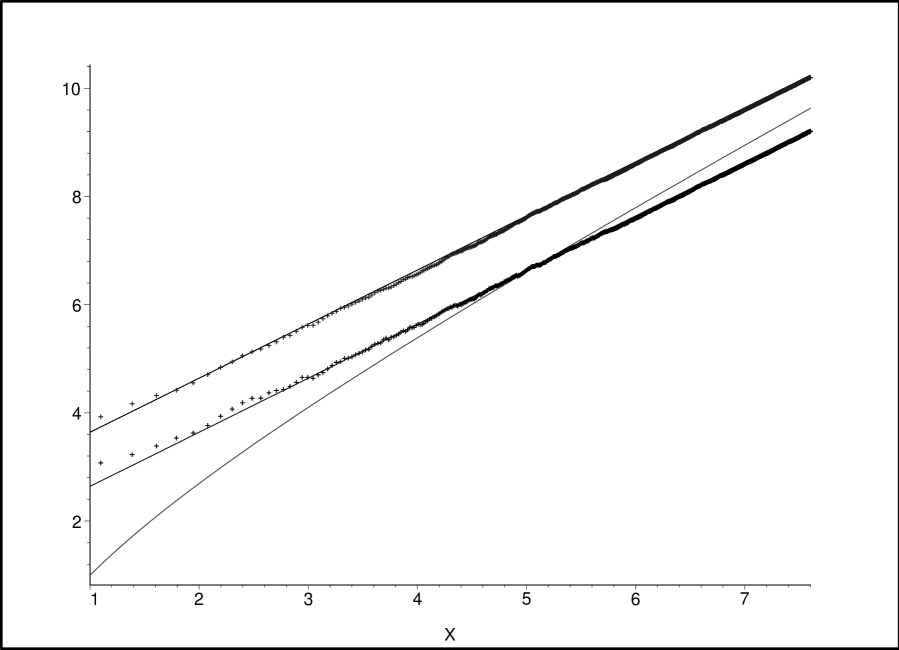
Figure 3. Plot of $\log h(y_{n})$ (bottom set of points) and $\log h(z_{n})$ (top set of points) versus $\log n$ for the first 2000 iterates of the integrable map $d{\mathcal{E}}_{7}$ for $\epsilon=1/2$ with initial conditions $x_{0}=3/7,y_{0}=11/13,z_{0}=23/47$ and parameter $\xi=19/17$. The bottom points have been fitted against $\log n+1.64$ (a straight line on this scale), and the top points against $\log n+2.64$; the curve $\log n+\log\log n$ is also shown.

Finally, for the systems $d{\mathcal{E}}_{7}$ and $d{\mathcal{E}}_{8}$ we make use of direct estimates of the growth of heights, based on the original maps. For both these systems, note that from the explicit solution we have $h(x_{n})=h(n+\tau)=\log n+O(1)$. It is convenient to define $Y_{n}=y_{n}/x_{n}$ and $Z_{n}=z_{n}/x_{n}$ in each case, and then note that $h(y_{n})=h(Y_{n})+O(\log n)$, and similarly for $h(z_{n})$. From the second part of the map $d{\mathcal{E}}_{7}$ we have

$$Y_{n+1}=\left(\frac{n+\tau+1-\xi/2}{n+\tau+\xi/2}\right)\,Y_{n},$$ (54)

which implies

$$h(Y_{n+1})-h(Y_{n})\leq\log n+O(1)\implies h(Y_{n})\leq n\log n+O(n),$$

where the second implication follows by summing over $n$. Thus $h(Y_{n})$ has weaker than quadratic growth in $n$. Similarly for $Z_{n}$ we have

$$(n+\tau-1/2)Z_{n+1}=(n+\tau+3/2)Z_{n}+2\xi Y_{n}Y_{n+1},$$

which implies that

$$h(Z_{n+1})\leq h(Z_{n})+h(Y_{n}Y_{n+1})+O(\log n)\leq h(Z_{n})+n\log n+O(n),$$

and hence $h(Z_{n})\leq\frac{1}{2}n^{2}\log n+O(n^{2})$, which is weaker than cubic in $n$. For $d{\mathcal{E}}_{8}$, analogous estimates show that $h(Y_{n})\leq n\log n+O(n)$ and $h(Z_{n})\leq 2n^{2}\log n+O(n^{2})$, so this system is Diophantine integrable as well.

$\square$

Having proved that the systems are all Diophantine integrable, we can compare the theoretical results with some numerical experiments. For the system $d{\mathcal{E}}_{3}$ we see that the log-log plot gives what we expect: genus zero means linear growth of logarithmic height, so $\log h(x_{n})=\log n+O(1)$; this is evident from the plot of points in Figure 1, which lie asymptotically on a straight line of slope 1. Similarly for the genus one case, we expect $\log h(x_{n})=2\log n+O(1)$, and Figure 1 shows points which asymptote to a line with slope 2. In this case the offset, corresponding to the correction at $O(1)$, is function of the height of a point on an associated elliptic curve, and both the point and the curve vary with the initial data of the map.

Figure 4. Plot of $\log(h(x_{n})/n)$ versus $n$ for $d{\mathcal{E}}_{3}$ with the same data as Figure 1.

The theoretical results on the growth of heights for the algebraically integrable systems $d{\mathcal{E}}_{i}$ for $1\leq i\leq 6$, as detailed in the above proof, are confirmed by the numerical calculations, and for those cases we have an exact expression for the leading order asymptotic behaviour. Moreover, one can also look at how the asymptote is approached. Taking the system $d{\mathcal{E}}_{3}$ for example, $h(x_{n})/n$ approaches a constant as $n\to\infty$, and from the numerical plot in Figure 4 one can see that this limit is reached in a very uniform manner, in keeping with a correction of $O(1/n)$ to this constant. Similarly, in the case of $d{\mathcal{E}}_{4}$, corresponding to motion on an elliptic curve, we see from Figure 5 that once again the convergence of $h(x_{n})/n^{2}$ to a constant appears to be almost monotone.

Figure 5. Plot of $\log(h(x_{n})/n^{2})$ versus $n$ for $d{\mathcal{E}}_{4}$ with the same data as Figure 2.

The non-algebraically integrable cases, $d{\mathcal{E}}_{7}$ and $d{\mathcal{E}}_{8}$, have some extremely interesting features compared with the others. First of all, the method of proof used in Theorem 4 above has not necessarily provided the leading order asymptotics of the logarithmic heights, but has merely given upper bounds on the growth of the form $Cn^{j}\log n$ with $j=1$ for $h(y_{n})$ and $j=2$ for $h(z_{n})$ in each case. Let us focus on the case of $d{\mathcal{E}}_{7}$. Upon looking more closely at Eq. (54), it would appear that the upper bound for $h(Y_{n})$ might be sharp, so that $h(Y_{n})\sim n\log n$ (and $h(y_{n})$ would have the same leading order asymptotics). However, studies of particular sequences of rational iterates show that cancellations occur between the numerator and denominator of $Y_{n}$ and the prefactor $(n+\alpha+1-\xi/2)/(n+\alpha+\xi/2)$, which means that the height of $Y_{n+1}$ is therefore smaller than the crudest estimate for the upper bound. This weaker growth has a knock-on effect, meaning that the growth of heights of $z_{n}$ also seems to be much weaker than expected. Indeed, Figure 3 suggests that the correct asymptotics should be linear growth in $n$ for the logarithmic heights of both $y_{n}$ and $z_{n}$, i.e. $h(y_{n})\sim C_{1}n$ and $h(z_{n})\sim C_{2}n$ for positive constants $C_{1},C_{2}$. For the particular sequence of heights plotted in that figure, a numerical fit shows that $\log C_{1}\approx 1.64$ and $\log C_{2}\approx 2.64\approx\log C_{1}+1$. We have also plotted $\log n+\log\log n$ for comparison, to show how the upper bound for $h(y_{n})$ fails to be sharp. Another surprising feature of this system is that for different choices of initial data we find (to within numerical accuracy) the same values of $C_{1}$ and $C_{2}$; this is in contrast to the algebraically integrable setting described above, where the coefficient in front of the leading order term is dependent on the initial data. Thus we might conjecture that for this map $C_{1},C_{2}$ are independent of initial data, and also that $C_{2}=e\,C_{1}$ holds identically, in which case there should be some deeper arithmetical explanation for this asymptotic behaviour. Similarly to the case of $d{\mathcal{E}}_{7}$, numerical results for the system $d{\mathcal{E}}_{8}$ also show linear growth of logarithmic heights.

Figure 6. Plot of 400 iterates of $\log(h(x_{n})/n)$ versus $n$ for $d{\mathcal{E}}_{7}$ with the same initial data and parameters as in Figure 3.

Supposing that the numerical observation of linear growth of $h_{n}$ for these discrete systems with transcendental invariants is indeed the correct asymptotic behaviour, it is then interesting to look at how $h_{n}/n$ approaches a constant value. The results we find are in stark contrast to the algebraic setting: rather than the almost monotone convergence seen in the previous examples, for $d{\mathcal{E}}_{7}$ we find that $h_{n}/n$ shows rapid fluctuations which persist for increasing values of $n$. These fluctuations in the asymptotics are somewhat reminiscent of the “random”-looking error terms that appear in some famous arithmetical functions, such as the difference between the prime-counting function $\pi(n)$ and the logarithmic integral [25]. It would be interesting to know whether these fluctuations might provide a means of characterizing the difference between discrete systems which are algebraically integrable and those with transcendental invariants.

Figure 7. Plot of $\log h(x_{n})$ versus $\log n$ for the first 17 iterates of Kahan’s discretization of the Lotka-Volterra system with initial conditions $x_{0}=1/2,y_{0}=5/3$ and parameter $\epsilon=9/14$.

For comparison with the Diophantine integrable examples above, in Figure 7 above we have plotted the growth of $h_{n}$ for a particular case of the discrete Lotka-Volterra system due to Kahan, which is the degree two birational map given in Eq. (2). This figure shows that the logarithmic height seems to grow exponentially, indicating non-integrability of this system. Indeed, the heights of iterates grow so fast that even on a fairly new computer it took 1 hour to calculate the heights of 17 rational iterates with Maple; the value of $h(x_{17})$ is of the order of $10^{325009}$ in this case. Upon examining the data used in Figure 7 more carefully, it is apparent that $h(x_{n+1})\approx 2\,h(x_{n})$ to very good accuracy, so we expect $h_{n}\sim C\,2^{n}$. This would mean that the logarithmic height essentially doubles with each step, giving a Diophantine entropy of $\log 2$ for generic (aperiodic) orbits. This appears to be the same as the algebraic entropy of the map when $\epsilon^{2}\neq 1$, which was calculated by A. Ramani [33]. In any case, this is the entropy value that one would expect for a generic (non-integrable) birational map of degree two.

Finally we should mention the results of numerical calculations of the growth of heights for the map $d{\mathcal{E}}_{9}$ for various cases with $\xi\neq\pm 1$ (that is, excluding the two special cases where the map is already known to be algebraically integrable). For generic rational values of the parameter $\xi$ we find that the map $d{\mathcal{E}}_{9}$ is not Diophantine integrable, but rather the Diophantine entropy is $\log 3$ for generic orbits, this being the typical value to be expected for a non-integrable birational map of degree three. (See Figure 8 for an illustration of the exponential growth of logarithmc heights when $\xi=-1/2$.) These numerical results suggest that while that the original continuous system ${\mathcal{E}}_{9}$ is algebraically integrable (in the sense of having two independent algebraic integrals), the corresponding discrete system is not. We shall return to this point in our conclusions.

Figure 8. Plot of $\log h(x_{n})$ versus $\log n$ for the first 11 iterates of the map $d{\mathcal{E}}_{9}$ for $\epsilon=1/2$ with initial conditions $x_{0}=2/5,y_{0}=7/3,z_{0}=11/13$ and parameter $\xi=-1/2$.

8. Concluding remarks

In this paper we studied three-dimensional birational maps which provide integrable time-discretizations of quadratic bi-Hamiltonian flows associated with pairs of real three-dimensional Lie algebras, as presented in [3, 11]. We have shown that for the six cases of continuous flows which are algebraically integrable, the Hirota-Kimura type discretization provides maps admitting two independent rational integrals of motion, in involution with respect to a pair of compatible Poisson tensors. We have also provided explicit solutions of the resulting discrete systems $d{\mathcal{E}}_{i}$ for $i=1,\ldots,6$, which are given in terms of either rational, hyperbolic or elliptic functions in each case. These results confirm the conjecture that the property of algebraic integrability is preserved by this discretization scheme.

We have also applied the same procedure to two cases of integrable continuous flows in three dimensions having one rational and one transcendental integral of motion, for which the resulting maps, $d{\mathcal{E}}_{7}$ and $d{\mathcal{E}}_{8}$, admit explicit solutions in terms of rational functions and either gamma or digamma functions. In each of these cases, we have found an explicit formula for one transcendental integral of the map, but the second integral is only defined implicitly by the solution. Nevertheless, this is sufficient to assert that the latter two cases are also completely integrable in the Liouville-Arnold sense. Therefore the Kahan-Hirota-Kimura discretization scheme preserves integrability even in these transcendental cases. However, for another example of a continuous integrable system with one transcendental integral, it appears likely that the corresponding discretization $d{\mathcal{E}}_{9}$ is not integrable for generic values of the parameter in the map.

In an attempt to gain a better understanding of the difference between the algebraic and transcendental cases, we have also analyzed all of these discrete systems from a different viewpoint, within the arithmetical setting of Diophantine integrability. So far, the Diophantine integrability test has been applied to various algebraically integrable systems and discrete Painlevé equations [12], as well as to certain birational maps that are not algebraically integrable and fail the test [18, 19]. Our theoretical results show that $d{\mathcal{E}}_{7}$ and $d{\mathcal{E}}_{8}$ provide examples of discrete integrable systems with transcendental invariants that are also Diophantine integrable, in the sense defined by Halburd. Moreover, more detailed numerical results suggest that these discrete integrable systems might be distinguished from algebraically integrable maps by the manner in which the logarithmic heights converge to their leading order asymptotics. This asymptotic behaviour deserves to be studied more carefully in the future.

A further interesting point is the comparison with Kahan’s discretization of the Lotka-Volterra system, which is an integrable flow in the plane with a transcendental integral. The discrete system provides a non-standard symplectic integrator of this flow, and seems to preserve the qualitative features of the continuous counterpart. However, the numerical results indicate that the discrete system is not Diophantine integrable, which adds further evidence to the conjecture that (for generic values of $\epsilon$) it should not be Liouville integrable either.

Similar considerations apply to the discrete system $d{\mathcal{E}}_{9}$: numerically it appears that for generic values of the parameter $\xi$, it fails the Diophantine integrability test. Since the continuous system ${\mathcal{E}}_{9}$ has algebraic integrals for $\xi\in\mathbb{Q}$, this means that in general algebraic integrability (in the weakest sense of the term) is not preserved by the Kahan-Hirota-Kimura discretization. Actually one could already observe this for the system ${\mathcal{E}}_{7}$, since it has the integral $H_{7}$ which is algebraic for all $\xi\in\mathbb{Q}$, but the integral $\widehat{H}_{7}$ for $d{\mathcal{E}}_{7}$ is transcendental unless $\xi\in\mathbb{Z}$. This suggests that one should impose a much stronger notion of algebraic complete integrability (a.c.i.) if this is to be preserved by the discretization scheme. For instance, one can require that the generic level sets of the integrals are smooth abelian varieties, possibly extended by $(\mathbb{C}^{*})^{m}$ for some $m$. An excellent discussion of various different definitions of a.c.i. can be found in chapter V of [40].

As for the case of the discrete three-dimensional Euler top (see [15, 30]), there is one other standard attribute of integrable systems that remains to be found for the maps $d{\mathcal{E}}_{i}$ for $i=1,\ldots,8$, namely their Lax representation. This is an open problem which deserves further investigation.

There are three other bi-Hamiltonian flows in the list of Gümral and Nutku, all of which have one transcendental invariant. Preliminary results suggest that their Kahan-Hirota-Kimura type discretizations are qualitatively similar to the system $d{\mathcal{E}}_{9}$, and we expect that these maps are not Liouville integrable. We reserve the study of these systems for future work.

Finally we remark that another non-standard symplectic integrator for the Lotka-Volterra model, with similar numerical properties, has been given by Mickens in [26]. It would be very interesting to see if the approach to discretization proposed by Mickens shares some of the remarkable properties of Kahan’s.

Appendix: solution of the system $d{\mathcal{E}}_{4}$ in elliptic functions

Here we derive the formulae (27-29) corresponding to the solution of $d{\mathcal{E}}_{4}$, as in Theorem 3. The first observation to make is that the curve ${\mathcal{V}}$ in affine three-dimensional space defined by the equations

$${\mathcal{V}}:\qquad xy=H\left[1+\epsilon^{2}(x^{2}+y^{2})\right],\qquad x^{2}+y^{2}+z^{2}=2K\left[1+\epsilon^{2}(x^{2}+y^{2})\right],$$

corresponding to the intersection of the level sets $\widehat{H}_{4}=H$, $\widehat{K}_{4}=K$, has genus one (at least for generic values of $H$ and $K$). To see this, note that ${\mathcal{V}}$ is a double cover of the curve

$${\mathcal{C}}:\qquad xy=H\left[1+\epsilon^{2}(x^{2}+y^{2})\right]$$

in two dimensions, via the covering map

$$\begin{array}[]{lccc}\pi:&{\mathcal{V}}&\rightarrow&{\mathcal{C}}\\ &(x,y,z)&\mapsto&(x,y)\end{array}$$

which is ramified over the four points $(x,y)\in{\mathcal{C}}$ obtained from the simultaneous solutions of $xy=H(1+\epsilon^{2}(x^{2}+y^{2}))$, $(1-2K\epsilon^{2})(x^{2}+y^{2})=2K$ (when $z=0$). Since the curve ${\mathcal{C}}$ is a conic (genus zero), it follows from the Riemann-Hurwitz formula [27] that ${\mathcal{V}}$ is (the affine part of) a curve of genus one. The first order recurrence relations for $x_{n},y_{n},z_{n}$, namely

$$x_{n+1}-x_{n}=-\epsilon(x_{n+1}z_{n}+x_{n}z_{n+1}),$$ (55)

$$y_{n+1}-y_{n}=\epsilon(y_{n+1}z_{n}+y_{n}z_{n+1}),$$ (56)

$$z_{n+1}-z_{n}=2\epsilon(x_{n+1}x_{n}-y_{n}y_{n+1}),$$ (57)

correspond to a birational map from this curve to itself, inducing an automorphism of an isomorphic elliptic curve (i.e. a plane curve defined by a Weierstrass cubic), and it follows that $x_{n}=X(u+nv)$ for a suitable elliptic function $X$, and similarly for $y_{n},z_{n}$. One can see some points on a real connected component of such a curve in Figure 9.

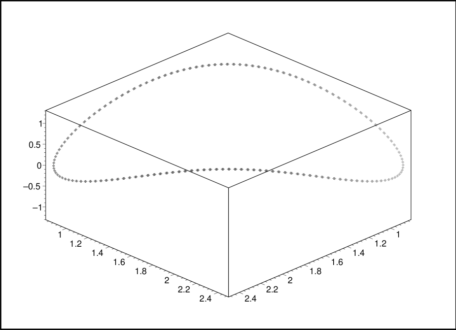
Figure 9. Plot of the first 1000 points on the orbit of the integrable map $d{\mathcal{E}}_{4}$ with initial conditions $x_{0}=7/3,y_{0}=11/13,z_{0}=23/47$.

From the equations for ${\mathcal{V}}$ it is easy to see that the functions corresponding to $x_{n},y_{n},z_{n}$ each have simple poles at the same places, and they are elliptic functions of order two. These facts suggest that it may be most convenient to write the formulae in terms of Jacobian (rather than Weierstrassian) elliptic functions. Indeed, if we set

$$s=x+y,\qquad d=x-y,$$

then the equations for ${\mathcal{V}}$ become

$$(1-2H\epsilon^{2})s^{2}-(1+2H\epsilon^{2})d^{2}=4H,\qquad(1-2K\epsilon^{2})(s^{2}+d^{2})+4z^{2}=4K,$$

which are reminiscent of (linear combinations of) the quadratic relations

$${\mathrm{sn}}^{2}(u)+{\mathrm{cn}}^{2}(u)=1,\qquad k^{2}{\mathrm{sn}}^{2}(u)+{\mathrm{dn}}^{2}(u)=1,$$

for Jacobi functions.

In order to obtain the formulae (27-29), it is instructive to take a detour through Jacobi theta functions, by deriving bilinear equations from Eqs. (55-57). Upon setting

$$x_{n}=\frac{A_{n}+B_{n}}{2\epsilon D_{n}},\qquad y_{n}=\frac{A_{n}-B_{n}}{2\epsilon D_{n}},\qquad z_{n}=\frac{C_{n}}{\epsilon D_{n}},$$

the system (55) is equivalent to the following three bilinear equations:

$$\left\{\begin{array}[]{l}A_{n+1}D_{n}-A_{n}D_{n+1}=-(B_{n+1}C_{n}+B_{n}C_{n+1}),\\ B_{n+1}D_{n}-B_{n}D_{n+1}=-(A_{n+1}C_{n}+A_{n}C_{n+1}),\\ C_{n+1}D_{n}-C_{n}D_{n+1}=A_{n+1}B_{n}+A_{n}B_{n+1}.\end{array}\right.$$ (58)

One should hesitate to call (58) the Hirota bilinear form of Eqs. (55-57), because there are four unknowns (tau-functions) $A_{n},B_{n},C_{n},D_{n}$ but only three equations, so the system is underdetermined. Despite this apparent problem, we can solve this bilinear system in terms of Jacobi theta functions $\vartheta_{j}$, $j=1,\ldots,4$, by comparing these equations with the identities in exercise number 3 on page 488 of [42]; the first of these is the relation

$$\vartheta_{1}(u\pm v)\vartheta_{2}(u\mp v)\vartheta_{3}\vartheta_{4}=\vartheta_{1}(u)\vartheta_{2}(u)\vartheta_{3}(v)\vartheta_{4}(v)\pm\vartheta_{3}(u)\vartheta_{4}(u)\vartheta_{1}(v)\vartheta_{2}(v)\,$$ (59)

the last is

$$\vartheta_{3}(u\pm v)\vartheta_{4}(u\mp v)\vartheta_{3}\vartheta_{4}=\vartheta_{3}(u)\vartheta_{4}(u)\vartheta_{3}(v)\vartheta_{4}(v)\mp\vartheta_{1}(u)\vartheta_{2}(u)\vartheta_{1}(v)\vartheta_{2}(v)\,$$ (60)

and there are four other relations of this kind, for different permutations of the four indices. Here $\vartheta_{j}$ without argument denotes a theta constant (i.e. $\vartheta_{j}=\vartheta_{j}(0)$, which depends on the modulus $k$). By taking the sum of the two equations given in (59) with opposite choices of $\pm$ signs, and similarly taking the difference of the two equations specified by (60), one sees that both $\vartheta_{1}(u+v)\vartheta_{2}(u-v)+\vartheta_{1}(u-v)\vartheta_{2}(u+v)$ and $\vartheta_{3}(u+v)\vartheta_{4}(u-v)-\vartheta_{3}(u-v)\vartheta_{4}(u+v)$ are proportional to $\vartheta_{1}(u)\vartheta_{2}(u)$, modulo $v$-dependent factors. Thus if $v$ is regarded as a fixed constant, and the shift $u\to u+2v$ is identified with $n\to n+1$, then the first equation in (58) is satisfied if (suppressing all arguments and the index $n$) the identifications

$$C\sim\vartheta_{1},\quad B\sim\vartheta_{2},\quad A\sim\vartheta_{3},\quad D\sim\vartheta_{4}$$

are made, up to suitable $v$-dependent scaling denoted by the $\sim$ symbol. Moreover, these identifications are consistent with the second and third equations in (58), which are consequences of the aforementioned other four bilinear relations between Jacobi theta functions.

Given that the Jacobian elliptic functions are defined in terms of theta functions by

$${\mathrm{sn}}(u)=\frac{\vartheta_{3}}{\vartheta_{2}}\frac{\vartheta_{1}(u/\vartheta_{3}^{2})}{\vartheta_{4}(u/\vartheta_{3}^{2})},\qquad{\mathrm{cn}}(u)=\frac{\vartheta_{4}}{\vartheta_{2}}\frac{\vartheta_{3}(u/\vartheta_{3}^{2})}{\vartheta_{4}(u/\vartheta_{3}^{2})},\qquad{\mathrm{dn}}(u)=\frac{\vartheta_{4}}{\vartheta_{3}}\frac{\vartheta_{3}(u/\vartheta_{3}^{2})}{\vartheta_{4}(u/\vartheta_{3}^{2})},\qquad$$

it follows that the solution of the difference equations (55) has the form

$$x_{n}=\lambda\,{\mathrm{dn}}(\kappa+2n\delta)+\mu\,{\mathrm{cn}}(\kappa+2n\delta),$$

$$y_{n}=\lambda\,{\mathrm{dn}}(\kappa+2n\delta)-\mu\,{\mathrm{cn}}(\kappa+2n\delta),$$

$$z_{n}=\nu\,{\mathrm{sn}}(\kappa+2n\delta),$$

for constants $\delta,\kappa$ and suitable prefactors $\lambda,\mu,\nu$ which are given in terms of $\delta$ and the theta constants. The expressions (27-29) can also be verified directly from the addition formula for ${\mathrm{sn}}$, namely

$${\mathrm{sn}}(u+v)=\frac{{\mathrm{sn}}(u){\mathrm{cn}}(v){\mathrm{dn}}(v)+{\mathrm{sn}}(v){\mathrm{cn}}(u){\mathrm{dn}}(u)}{1-k^{2}{\mathrm{sn}}^{2}(u){\mathrm{sn}}^{2}(v)},$$ (61)

as well as the analogous formulae for ${\mathrm{cn}}$ and ${\mathrm{dn}}$. Using (61) to calculate ${\mathrm{sn}}(u+v)-{\mathrm{sn}}(u-v)$, and then setting $u\to\kappa+(2n+1)\delta$, $v\to\delta$, gives an expression for the left hand side of the third equation in (55), and performing analogous computations for the right hand side and for the other two difference equations allows the prefactors $\lambda,\mu,\nu$ to be determined directly in terms of Jacobi functions with argument $\delta$, in agreement with (27-29).

Finally, note that the solution depends on the required number of arbitrary constants, namely the three parameters $\delta,\kappa,k$. The parameter $\delta$ and the modulus $k$ are determined by the values of the integrals $\widehat{H}_{4}$ and $\widehat{K}_{4}$, by solving the relations (30) as a system for $k$ and ${\mathrm{sn}}\delta$ and then performing the elliptic integral $\delta=\int_{0}^{{\mathrm{sn}}\delta}d\xi/\eta$, while $\kappa$ is found from

$$\kappa=\int_{0}^{\frac{\epsilon z_{0}}{k{\mathrm{sn}}\delta}}\frac{d\xi}{\eta},\qquad\eta^{2}=(1-\xi^{2})(1-k^{2}\xi^{2}).$$

References

• [1] Ablowitz M.J., Halburd R. and Herbst B., On the extension of the PainlevΓ© property to difference equations, Nonlin. 13 (2000) 889–905.
• [2] Adler M. and Van Moerbeke P., Geodesic flow on $SO(4)$ and the intersection of quadrics, Proc. Natl. Acad. Sci. USA 81 (1984) 4613–4616.
• [3] Blaszak M. and Wojciechowski S., Bi-Hamiltonian dynamical systems related to low-dimensional Lie algebras, Phys. A 155 (1989) 545–564.
• [4] Budd C.J. and Iserles A. (Eds.), Geometric integration: numerical solution of differential equations on manifolds, Phil. Trans. R. Soc. Lond. A 357 (1999) 943–1133.
• [5] Byrnes G.B., Haggar F.A. and Quispel G.R.W., Sufficient conditions for dynamical systems to have pre-symplectic or pre-implectic structures, Phys. A 272 (1999) 99–129.
• [6] Cassels J.W.S., Lectures on elliptic curves, London Mathematical Society Student Texts 24, Cambridge University Press (1991).
• [7] Dragovic V. and Gajic C., Hirota-Kimura type discretization of the classical nonholonomic Suslov problem; http://arxiv.org/abs/0807.2966.
• [8] Giacomini H.J., Integrable Hamiltonians with higher transcendental invariants, Jour. Phys. A: Math. Gen. 23 (1990) L587–L590.
• [9] Grabowski J., Marmo G. and Perelomov A.M., Poisson structures: towards a classification, Mod. Phys. Lett. A 8 18 (1993) 1719–1733.
• [10] Grammaticos B., Ramani A. and Papageorgiou V., Do integrable mappings have the PainlevΓ© property?, Phys. Rev. Lett. 67 (1991) 1825–1828.
• [11] GΓΌmral H. and Nutku Y., Poisson structure of dynamical systems with three degrees of freedom, Jour. Math. Phys. 34 12 (1993) 5691–5722.
• [12] Halburd R., Diophantine integrability, Jour. Phys. A: Math. Gen. 38 (2005) L263–L269.
• [13] Hietarinta J., New integrable Hamiltonians with transcendental Invariants, Phys. Rev. Lett. 52 13 (1984) 1057–1060.
• [14] Hietarinta J. and Viallet C., Singularity confinement and chaos in discrete systems, Phys. Rev. Lett. 81 (1998) 325–328.
• [15] Hirota R. and Kimura K., Discretization of the Euler top, Jour. Phys. Soc. Jap. 69 (2000) 627–630.
• [16] Hirota R., Kimura K. and Yahagi H., How to find the conserved quantities of nonlinear discrete equations, Jour. Phys. A: Math. Gen. 34 (2001) 10377–10386.
• [17] Holm D.D., Geometric mechanics. Part I: dynamics and symmetry, Imperial College Press, World Scientific (2008).
• [18] Hone A.N.W., Diophantine non-integrability of a third-order recurrence with the Laurent property, Jour. Phys. A: Math. Gen. 39 (2006) L171–L177.
• [19] Hone A.N.W., Singularity confinement for maps with the Laurent property, Phys. Lett. A 261 (2007) 341–345.
• [20] Kahan W., Unconventional numerical methods for trajectory calculations, Unpublished lecture notes (1993).
• [21] Kahan W. and Li R.-C., Unconventional schemes for a class of ordinary differential equations – with applications to the Korteweg-de Vries equation, Jour. Comp. Phys. 134 (1997), 316–331.
• [22] Kimura K. and Hirota R., Discretization of the Lagrange top, Jour. Phys. Soc. Jap. 69 (2000) 3193–3199.
• [23] Lafortune S. and Goriely A., Singularity confinement and algebraic integrability, Jour. Math. Phys. 45 3 (2004) 1191–1208.
• [24] Magri F. and Morosi C., A geometrical characterization of integrable Hamiltonian systems through the theory of Poisson-Nijenhuis manifolds, Quaderno 19/S, Dip. Mat. Univ. Milano, 1984.
• [25] Mazur B., Finding meaning in error terms, Bull. Amer. Math. Soc. 45 2 (2008) 185–228.
• [26] Mickens R.E., A nonstandard finite-difference scheme for the Lotka-Volterra system, Appl. Num. Math. 45 (2003) 309–314.
• [27] Miranda R., Algebraic curves and Riemann surfaces, Graduate Studies in Mathematics 5, American Mathematical Society, Providence, RI, 1995.
• [28] Nambu Y., Generalized Hamiltonian dynamics, Phys. Rev. D 7 8 (1973) 2405–2412.
• [29] Patera J., Sharp R.T., Winternitz P. and Zassenhaus H., Invariants of real low dimensional Lie algebras, Jour. Math. Phys. 17 6 (1976) 986–994.
• [30] Petrera M. and Suris Yu.B., On the Hamiltonian structure of Hirota-Kimura discretization of the Euler top, to appear in Math. Nach.; http://arxiv.org/abs/0707.4382.
• [31] Petrera M. and Suris Yu.B., Hirota-type discretization of 2d Lotka-Volterra system, preprint (2007).
• [32] Petrera M., Pfadler A. and Suris Yu.B., On integrability of Hirota-Kimura type discretizations. Experimental study of the discrete Clebsch system, to appear in Exp. Math.; http://arxiv.org/abs/0808.3345.
• [33] Ramani A., private communication to Yu.B. Suris (2007).
• [34] Reyman A.G. and Semenov-Tian-Shansky M.A., Group theoretical methods in the theory of finite-dimensional integrable systems, in Dynamical systems VII, Springer, 1994.
• [35] Roberts J.A.G. and Vivaldi F., Arithmetical method to detect integrability in maps, Phys. Rev. Lett. 90 (2003) 034102.
• [36] Roeger L.W., A nonstandard discretization method for Lotka-Volterra models that preserves periodic solutions, Jour. Diff. Eq. Appl. 11 (2005) 721–733. Roeger L.W., Discrete May-Leonard competition models III, Jour. Diff. Eq. Appl. 10 (2004) 773–790.
• [37] Sanz-Serna, J. M., An unconventional symplectic integrator of W. Kahan, Appl. Num. Math. 16 (1994) 245–250.
• [38] Silverman J., The Arithmetic of Elliptic Curves, Springer, 1986.
• [39] Suris Yu.B., The problem of integrable discretization: Hamiltonian approach, Progress in Mathematics, 219, BirkhΓ€user Verlag, Basel, 2003.
• [40] Vanhaecke P., Integrable systems in the realm of algebraic geometry, 2nd Edition, Springer, 2001.
• [41] Veselov A.P., Integrable maps, Russ. Math. Surv. 46 (1991) 1–51.
• [42] Whittaker E.T. and Watson G.N., A course of modern analysis, 4th edition, Cambridge University Press, 1927.
• [43] Willox R., Grammaticos B. and Ramani A., Jour. Phys. A 38 (2005) 5227–5236.