The Magnus expansion and some of its applications

Abstract

Approximate resolution of linear systems of differential equations with varying coefficients is a recurrent problem shared by a number of scientific and engineering areas, ranging from Quantum Mechanics to Control Theory. When formulated in operator or matrix form, the Magnus expansion furnishes an elegant setting to built up approximate exponential representations of the solution of the system. It provides a power series expansion for the corresponding exponent and is sometimes referred to as Time-Dependent Exponential Perturbation Theory. Every Magnus approximant corresponds in Perturbation Theory to a partial re-summation of infinite terms with the important additional property of preserving at any order certain symmetries of the exact solution.

The goal of this review is threefold. First, to collect a number of developments scattered through half a century of scientific literature on Magnus expansion. They concern the methods for the generation of terms in the expansion, estimates of the radius of convergence of the series, generalizations and related non-perturbative expansions. Second, to provide a bridge with its implementation as generator of especial purpose numerical integration methods, a field of intense activity during the last decade. Third, to illustrate with examples the kind of results one can expect from Magnus expansion in comparison with those from both perturbative schemes and standard numerical integrators. We buttress this issue with a revision of the wide range of physical applications found by Magnus expansion in the literature.

, , and

1 Introduction

1.1 Motivation, overview and history

The outstanding mathematician Wilhelm Magnus (1907-1990) did important contributions to a wide variety of fields in mathematics and mathematical physics [1]. Among them one can mention combinatorial group theory [159] and his collaboration in the Bateman project on higher transcendental functions and integral transforms [81]. In this report we review another of his long-lasting constructions: the so-called Magnus expansion (hereafter referred to as ME). ME was introduced as a tool to solve non-autonomous linear differential equations for linear operators. It is interesting to observe that in his seminal paper of 1954 [158], although it is essentially mathematical in nature, Magnus recognizes that his work was stimulated by results of K.O. Friedrichs on the theory of linear operators in Quantum Mechanics [88]. Furthermore, as the first antecedent of his proposal he quotes a paper by R.P. Feynman in the Physical Review [86]. We stress these facts to show that already in its very beginning ME was strongly related to Physics and so has been ever since and there is no reason to doubt that it will continue to be. This is the first motivation to offer here a review as the present one.

Magnus proposal has the very attractive property of leading to approximate solutions which exhibit at any order of approximation some qualitative or physical characteristics which first principles guarantee for the exact (but unknown) solution of the problem. Important physical examples are the symplectic or unitary character of the evolution operator when dealing with classical or quantum mechanical problems, respectively. This is at variance with most standard perturbation theories and is apparent when formulated in a correct algebraic setting: Lie algebras and Lie groups. But this great advantage has been some times darkened in the past by the difficulties both in constructing explicitly higher order terms and in assuring existence and convergence of the expansion.

In our opinion, recent years have witnessed great improvement in this situation. Concerning general questions of existence and convergence new results have appeared. From the point of view of applications some new approaches in old fields have been published while completely new and promising avenues have been open by the use of Magnus expansion in Numerical Analysis. It seems reasonable to expect fruitful cross fertilization between these new developments and the most conventional perturbative approach to ME and from it further applications and new calculations.

This new scenario makes desirable for the Physics community in different areas (and scientists and engineers in general) to have access in as unified a way as possible to all the information concerning ME which so far has been treated in very different settings and has appeared scattered through very different bibliographic sources.

As implied by the preceding paragraphs this report is mainly addressed to a Physics audience, or closed neighbors, and consequently we shall keep the treatment of its mathematical aspects within reasonable limits and refer the reader to more detailed literature where necessary. By the same token the applications presented will be limited to examples from Physics or from the closely related field of Physical Chemistry. We shall also emphasize its instrumental character for numerically solving physical problems.

In the present section as an introduction we present a brief overview and sketchy history of more than 50 years of ME. To start with, let us consider the initial value problem associated with the linear ordinary differential equation

$$Y^{\prime}(t)=A(t)Y(t),\qquad\qquad Y(t_{0})=Y_{0},$$ (1)

where as usual the prime denotes derivative with respect to the real independent variable which we take as time $t$, although much of what will be said applies also for a complex independent variable. In order of increasing complexity we may consider the equation above in different contexts:

1. $Y:\mathbb{R}\longrightarrow\mathbb{C}$, $A:\mathbb{R}\longrightarrow\mathbb{C}$. This means that the unknown $Y$ and the given $A$ are complex scalar valued functions of one real variable. In this case there is no problem at all: the solution reduces to a quadrature and an ordinary exponential evaluation:

   $$Y(t)=\exp\left(\int_{t_{0}}^{t}A(s)ds\right)\,Y_{0}.$$ (2)

2. $Y:\mathbb{R}\longrightarrow\mathbb{C}^{n}$, $A:\mathbb{R}\longrightarrow\mathbb{M}_{n}(\mathbb{C)}$, where $\mathbb{M}_{n}(\mathbb{C)}$ is the set of $n\times n$ complex matrices. Now $Y$ is a complex vector valued function and $A$ a complex $n\times n$ matrix valued function. At variance with the previous case, only in very special cases is the solution easy to state: when for any pair of values of $t$, $t_{1}$ and $t_{2},$ one has $A(t_{1})A(t_{2})=A(t_{2})A(t_{1})$, which is certainly the case if $A$ is constant. Then the solution reduces to a quadrature (trivial or not) and a matrix exponential. With the obvious changes in the meaning of the symbols, equation (2) still applies. In the general case, however, there is not compact expression for the solution and (2) is not any more the solution.

3. $Y:\mathbb{R}\longrightarrow\mathbb{M}_{n}(\mathbb{C)}$, $A:\mathbb{R}\longrightarrow\mathbb{M}_{n}(\mathbb{C)}$. Now both $Y$ and $A$ are complex matrix valued functions. A particular case, but still general enough to encompass the most interesting physical and mathematical applications, corresponds to $Y(t)\in\mathcal{G}$, $A(t)\in\mathfrak{g}$, where $\mathcal{G}$ and $\mathfrak{g}$ are respectively a matrix Lie group and its corresponding Lie algebra. Why this is of interest is easy to grasp: the key reason for the failure of (2) is the non-commutativity of matrices in general. So one can expect that the (in general non-vanishing) commutators play an important role. But when commutators enter the play one immediately thinks in Lie structures. Furthermore, plainly speaking, the way from a Lie algebra to its Lie group is covered by the exponential operation. A fact that will be no surprise in this context. The same comments of the previous case are valid here. In this report we shall mostly deal with this matrix case.

4. The most general situation one can think of corresponds to $Y(t)$ and $A(t)$ being operators in some space, e.g., Hilbert space in Quantum Mechanics. Perhaps the most paradigmatic example of (1) in this setting is the time-dependent Schrödinger equation.

Observe that case (b) above can be reduced to case (c). This is easily seen if one introduces what in mathematical literature is named the matrizant, a concept dating back at least to the beginning of the 20th century in the work of Baker [8]. It is the $n\times n$ matrix $U(t,t_{0})$ defined through

$$Y(t)=U(t,t_{0})Y_{0}.$$ (3)

Without loss of generality we will take $t_{0}=0$ unless otherwise explicitly stated, for the sake of simplicity. When no confusion may arise, we write only one argument in $U$ and denote $U(t,0)\equiv U(t)$, which then satisfy the differential equation and initial condition

$$U^{\prime}(t)=A(t)U(t),\qquad\qquad U(0)=I,$$ (4)

where $I$ stands for the $n$-dimensional identity matrix. The reader will have recognized $U(t)$ as what in physical terms is known as time evolution operator.

We are now ready to state Magnus proposal: a solution to (4) which is a true matrix exponential

$$U(t)=\exp\Omega(t),\qquad\qquad\Omega(0)=O,$$ (5)

and a series expansion for the matrix in the exponent

$$\Omega(t)=\sum_{k=1}^{\infty}\Omega_{k}(t),$$ (6)

which is what we call the Magnus expansion. The mathematical elaborations explained in the next section determine $\Omega_{k}(t)$. Here we just write down the three first terms of that series:

$$\Omega_{1}(t) =\int_{0}^{t}A(t_{1})~{}\text{d}t_{1},$$

$$\Omega_{2}(t) =\frac{1}{2}\int_{0}^{t}\text{d}t_{1}\int_{0}^{t_{1}}\text{d}t_{2}\ \left[A(t_{1}),A(t_{2})\right]$$ (7)

$$\Omega_{3}(t) =\frac{1}{6}\int_{0}^{t}\text{d}t_{1}\int_{0}^{t_{1}}\text{d}t_{2}\int_{0}^{t_{2}}\text{d}t_{3}\ (\left[A(t_{1}),\left[A(t_{2}),A(t_{3})\right]\right]+\left[A(t_{3}),\left[A(t_{2}),A(t_{1})\right]\right])$$

where $\left[A,B\right]\equiv AB-BA$ is the matrix commutator of $A$ and $B$.

The interpretation of these equations seems clear: $\Omega_{1}(t)$ coincides exactly with the exponent in (2). But this equation cannot give the whole solution as has already been said. So, if one insists in having an exponential solution the exponent has to be corrected. The rest of the ME in (6) gives that correction necessary to keep the exponential form of the solution.

The terms appearing in (7) already suggest the most appealing characteristic of ME. Remember that a matrix Lie algebra is a linear space in which one has defined the commutator as the second internal composition law. If, as we suppose, $A(t)$ belongs to a Lie algebra $\mathfrak{g}$ for all $t$ so does any sum of multiple integrals of nested commutators. Then, if all terms in ME have a structure similar to that of the ones shown before, the whole $\Omega(t)$ and any approximation to it obtained by truncation of ME will also belong to the same Lie algebra. In the next section it will be shown that this turns out to be the case. And a fortiori its exponential will be in the corresponding Lie group.

Why is this so important for physical applications? Just because many of the properties of evolution operators derived from first principles are linked to the fact that they belong to a certain Lie group: e.g. unitary group in Quantum Mechanics, symplectic group in Classical Mechanics. In that way use of (truncated) ME leads to approximations which share with the exact solution of equation (4) important qualitative (very often, geometric) properties. For instance, in Quantum Mechanics every approximant preserves probability conservation.

From the present point of view we could say that the last paragraphs summarize, in a nut shell, the main contents of the famous paper of Magnus of 1954. With no exaggeration its appearance can be considered a turning point in the treatment of the initial value problem defined by (4).

But important, as it certainly was, Magnus paper left some problems, at least partially, open:

• First, for what values of $t$ and for what operators $A$ does equation (4) admit a true exponential solution? This we call the existence problem.

• Second, for what values of $t$ and for what linear operators $A$ does the series in equation (6) converge? This we describe as the convergence problem. We want to emphasize that, although related, these two are different problems. To see why, think of the scalar equation $y^{\prime}=y^{2}$ with $y(0)=1$. Its solution $y(t)=(1-t)^{-1}$ exists for $t\neq 1$, but its form in power series $y(t)=\sum_{0}^{\infty}t^{n}$ converges only for $\left|t\right|<1$.

• Third, how to construct higher order terms $\Omega_{k}(t)$, $k\geq 3$, in the series? Moreover, is there a closed-form expression for $\Omega_{k}(t)$?

• Fourth, how to calculate in an efficient way $\exp\Omega^{[N]}$, where $\Omega^{[N]}\equiv\sum_{k=1}^{N}\Omega_{k}(t)$ is a truncation of the ME?

All these questions, and many others, will be dealt with in the rest of the paper. But before entering that analysis we think interesting to present a view, however brief, from a historical perspective of this half a century of developments on Magnus series. Needless to say, we by no means try to present a detailed and exhaustive chronological account of the many approaches followed by authors from very different disciplines. To minimize duplication with later sections we simply mention some representative samples in order the reader can understand the evolution of the field.

Including some precedents, and with a, as undeniable as unavoidable, dose of arbitrariness, we may distinguish four periods in the history of our topic:

1. Before 1953. The problem which ME solves has a centennial history dating back at least to the work of Peano, by the end of 19th century, and Baker, at the beginning of the 20th (for references to the original papers see e.g. [110]). They combine the theory of differential equations with an algebraic formulation. Intimately related to these treatments from the very beginning is the study of the so called Baker–Campbell–Hausdorff or BCH formula for short [9, 40, 102] which gives $C$ in terms of $A$, $B$ and their multiply nested commutators when expressing $\exp(A)\exp(B)$ as $\exp(C)$. This topic has by itself a long history up until today and will be discussed also in section 2. As one of its early hallmarks we quote [75]. In Physics literature the interest in the problem posed by equation (4) highly revived with the advent of Quantum Electrodynamics (QED). The works of F.J. Dyson [76] and in particular R.P. Feynman [86] in the late forties and early fifties are worth mentioning here.

2. 1953-1970. We have quoted as birth certificate of ME the paper [158] by Magnus in 1954. This is not strictly true: there is a Research Report [157] dated June 1953 which differs from the published paper in the title and in a few minor details and which should in fact be taken as a preliminary draft of it. In both publications appears the result summarized above on ME with almost identical words. The work of Pechukas and Light [195] gave for the first time a more specific analysis of the problem of convergence than the rather vague considerations in Magnus paper. Wei and Norman [235, 236] did the same for the existence problem. Robinson, to the best of our knowledge, seems to have been the first to apply ME to a physical problem [203]. Special mention in this period deserves a paper by Wilcox [239], in which useful mathematical tools are given and ME presented together with other algebraic treatments of equation (4), in particular Fer’s infinite product expansion [85]. Worth also of mention here is the first application of ME as a numerical tool for integrating the time-independent Schrödinger equation for potential scattering by Chang and Light [50].

3. 1971-1990. During these years ME consolidated in different fronts. It was successfully applied to a wide spectrum of fields in Physics and Chemistry: from atomic [11] and molecular [210] Physics to Nuclear Magnetic Resonance (NMR) [82, 234] to Quantum Electrodynamics [59] and elementary particle Physics [68]. A number of case studies also helped to clarify its mathematical structure, see for example [135]. The construction of higher order terms was approached from different angles. The intrinsic and growing complexity of ME allows for different schemes. One which has shown itself very useful in tackling other questions like the convergence problem was the recurrent scheme by Klarsfeld and Oteo [137].

4. Since 1991. The last decade of the 20th century witnessed a renewed interest in ME which still continues nowadays. It has followed different lines. Concerning the basic problems of existence and convergence of ME there has been definite progress [21, 43, 173, 176]. ME has also been adapted for specific types of equations: Floquet theory when $A(t)$ is a periodic function [45], stochastic differential equations [34] or equations of the form $Z^{\prime}=AZ-ZB$ [112]. Special mention should be made to the new field open in this most recent period that uses Magnus scheme to build novel algorithms [120] for the numerical integration of differential equations within the most wide field of geometric integration [32]. After optimization [22, 23], these integrators have proved to be highly competitive.

As a proof of the persistent impact the 1954 paper by Magnus has had in scientific literature we present in Figures 1 and 2 the number of citations per year and the cumulative number of citations, respectively, as December 2007 with data taken from ISI Web of Science. The original paper appears about 750 times of which, roughly, 50, 320 and 380 correspond respectively to each of the last three periods we have considered. The enduring interest in that seminal paper is clear from the figures.

Figure 1: Persistency of Magnus original paper: number of citations per year.

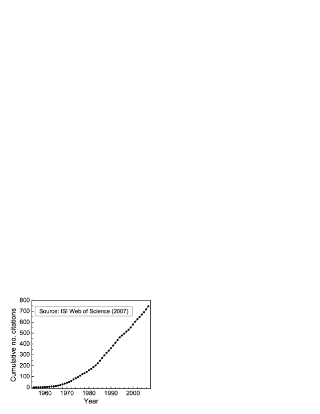
Figure 2: Persistency of Magnus original paper: cumulative number of citations.

The presentation of this report is organized as follows. In the remaining of this section we include some mathematical tools and notations that will be used time and again in our treatment. In section 2 we introduce formally the Magnus expansion, study its main features and analyze thoroughly the convergence issue. Next, in section 3 several generalizations of the Magnus expansion are reviewed, with special emphasis in its application to general nonlinear differential equations. In order to illustrate the main properties of ME, in section 4 we consider simple examples for which the computations required are relatively straightforward. Section 5 is devoted to an aspect that has been most recently studied in this setting: the design of new algorithms for the numerical integration of differential equations based on the Magnus expansion. There, after a brief characterization of numerical integrators, we present several methods that are particularly efficient, as shown by the examples considered. Given the relevance of the new numerical schemes, we briefly review in section 6 some of its applications in different contexts, ranging from boundary-value problems to stochastic differential equations. In section 7, on the other hand, applications of the ME to significant physical problems are considered. Finally, the paper ends with some concluding remarks.

1.2 Mathematical preliminaries and notations

Here we collect for the reader’s convenience some mathematical expressions, terminology and notations which appear most frequently in the text. Needless to say that we have made no attempt to being completely rigorous. We just try to facilitate the casual reading of isolated sections.

As already mentioned, the natural mathematical habitat for most of the objects we will deal with in this report is a Lie group or its associated Lie algebra. Although most of the results discussed in these pages are valid in a more general setting we will essentially consider only matrix Lie groups and algebras.

By a Lie group $\mathcal{G}$ we understand a set which combines an algebraic structure with a topological one. At the algebraic level every two elements of $\mathcal{G}$ can be combined by an internal composition law to produce a third element also in $\mathcal{G}$. The law is required to be associative, to have an identity element and every element must have an inverse. The ordinary product and inverse of invertible matrix play that role in the cases we are more interested in. The topological exigence forces the composition law and the association of an inverse to be sufficiently smooth functions.

A Lie algebra $\mathfrak{g}$ is a vector space whose elements can be combined by a second law, the Lie bracket, which we represent by $[A,B]=C$, with $A,B,C$ elements of $\mathfrak{g}$, in such a way that the law is bilinear, skew-symmetric and satisfies the well known Jacobi identity,

$$[A,[B,C]]+[B,[C,A]]+[C,[A,B]]=0.$$ (8)

When dealing with matrices we take as Lie bracket the familiar commutator:

$$[A,B]=AB-BA,\qquad A\in\mathfrak{g},\quad B\in\mathfrak{g},$$ (9)

where $AB$ stands for the usual matrix product. If we consider a finite-dimensional Lie algebra with dimension $d$ and denote by $A_{i},i=1,\ldots,d$, the vectors of one of its basis then the fundamental brackets one has to know are

$$[A_{i},A_{j}]=c_{ij}^{k}A_{k},$$ (10)

where sum over repeated indexes is understood. The coefficients $c_{ij}^{k}$ are the so-called structure constants of the algebra.

Associated with any $A\in\mathfrak{g}$ we can define a linear operator $\mathrm{ad}_{A}:\mathfrak{g}\rightarrow\mathfrak{g}$ which acts according to

$$\mathrm{ad}_{A}B=[A,B],\qquad\mathrm{ad}_{A}^{j}B=[A,\mathrm{ad}_{A}^{j-1}B],\qquad\mathrm{ad}_{A}^{0}B=B,\qquad j\in\mathbb{N},B\in\mathfrak{g}.$$ (11)

Also of interest is the exponential of this $\mathrm{ad}_{A}$ operator,

$$\mathrm{Ad}_{A}=\exp(\mathrm{ad}_{A}),$$ (12)

whose action on $\mathfrak{g}$ is given by

$$\mathrm{Ad}_{A}(B)=\exp(A)\,B\,\exp(-A)=\sum_{k=0}^{\infty}\frac{1}{k!}\mathrm{ad}_{A}^{k}B,\qquad B\in\mathfrak{g}.$$ (13)

The type of matrices we will handle more frequently are orthogonal, unitary and symplectic. Here are their characterization and the notation we shall use for their group and algebra.

The special orthogonal group, $\mathrm{SO}(n)$, is the set of all $n\times n$ real matrices with unit determinant satisfying $A^{T}A=AA^{T}=I$, where $A^{T}$ is the transpose of $A$ and $I$ denotes the identity matrix. The corresponding algebra $\mathfrak{so}(n)$ consists of the skew-symmetric matrices.

A $n\times n$ complex matrix $A$ is called unitary if $A^{{\dagger}}A=AA^{{\dagger}}=I$, where $A^{{\dagger}}$ is the conjugate transpose or Hermitian adjoint of $A$. The special unitary group, $\mathrm{SU}(n)$, is the set of all $n\times n$ unitary matrices with unit determinant. The corresponding algebra $\mathfrak{su}(n)$ consist of the skew-Hermitian traceless matrices. Special relevance in some quantum mechanical problems we discuss will have the case $n=2$. In this case a convenient basis for $\mathfrak{su}(2)$ is made up by the Pauli matrices

$$\sigma_{1}=\left(\begin{array}[]{ccr}0&&1\\ 1&&0\end{array}\right),\quad\sigma_{2}=\left(\begin{array}[]{ccr}0&&-i\\ i&&0\end{array}\right),\quad\sigma_{3}=\left(\begin{array}[]{ccr}1&&0\\ 0&&-1\end{array}\right).$$ (14)

They satisfy the identity

$$\sigma_{j}\sigma_{k}=\delta_{jk}+i\epsilon_{jkl}\sigma_{l},$$ (15)

and correspondingly

$$[\sigma_{j},\sigma_{k}]=2i\epsilon_{jkl}\sigma_{l},$$ (16)

which directly give the structure constants for $\mathrm{SU}(2)$. The following identities will prove useful for $\boldsymbol{a}$ and $\boldsymbol{b}$ in $\mathbb{R}^{3}$:

$$(\boldsymbol{a}\cdot\boldsymbol{\sigma})(\boldsymbol{b}\cdot\boldsymbol{\sigma})=\boldsymbol{a}\cdot\boldsymbol{b}\ I+i(\boldsymbol{a}\times\boldsymbol{b})\cdot\boldsymbol{\sigma},\qquad[\boldsymbol{a}\cdot\boldsymbol{\sigma},\boldsymbol{b}\cdot\boldsymbol{\sigma}]=2i(\boldsymbol{a}\times\boldsymbol{b})\cdot\boldsymbol{\sigma},$$ (17)

where we have denoted $\boldsymbol{\sigma}=(\sigma_{1},\sigma_{2},\sigma_{3})$. Any $U\in\mathrm{SU}(2)$ can be written as

$$U=\exp(i\boldsymbol{a}\cdot\boldsymbol{\sigma})=\cos(a)\,I+i\frac{\sin(a)}{a}\boldsymbol{a}\cdot\boldsymbol{\sigma},$$ (18)

where $a=\|\boldsymbol{a}\|=\sqrt{a_{1}^{2}+a_{2}^{2}+a_{3}^{2}}$. A more elaborate expression which we shall make use of in later sections is (with $a=1$)

$$\exp(i\boldsymbol{a}\cdot\boldsymbol{\sigma}t)\,(\boldsymbol{b}\cdot\boldsymbol{\sigma})\,\exp(-i\boldsymbol{a}\cdot\boldsymbol{\sigma}t)=\boldsymbol{b}\cdot\boldsymbol{\sigma}+\sin 2t\,(\boldsymbol{b}\times\boldsymbol{a})\cdot\boldsymbol{\sigma}+\sin^{2}t\,(\boldsymbol{a}\times(\boldsymbol{b}\times\boldsymbol{a}))\cdot\boldsymbol{\sigma}$$ (19)

In Hamiltonian problems the symplectic group $\mathrm{Sp}(n)$ plays a fundamental role. It is the group of $2n\times 2n$ real matrices satisfying

$$A^{T}JA=J,\qquad\mbox{ with }\quad\qquad J=\left(\begin{array}[]{rcc}O_{n}&&I_{n}\\ -I_{n}&&O_{n}\\ \end{array}\right)$$ (20)

and $I_{n}$ denotes the $n$-dimensional identity matrix. Its corresponding Lie algebra $\mathfrak{sp}(n)$ consists of matrices verifying $B^{T}J+JB=O_{2n}$. In fact, these can be considered particular instances of the so-called $J$-orthogonal group, defined as [197]

$$\mathrm{O}_{J}(n)=\{A\in\mathrm{GL}(n)\,:\,A^{T}JA=J\},$$ (21)

where $\mathrm{GL}(n)$ is the group of all $n\times n$ nonsingular real matrices and $J$ is some constant matrix in $\mathrm{GL}(n)$. Thus, one recovers the orthogonal group when $J=I$, the symplectic group $\mathrm{Sp}(n)$ when $J$ is the basic symplectic matrix given in (20), and the Lorentz group $\mathrm{SO}(3,1)$ when $J=\mathrm{diag}(1,-1,-1,-1)$. The corresponding Lie algebra is the set

$$\mathrm{o}_{J}(n)=\{B\in\mathfrak{gl}_{n}(\mathbb{R})\,:\,B^{T}J+JB=O\},$$ (22)

where $\mathfrak{gl}_{n}(\mathbb{R})$ is the Lie algebra of all $n\times n$ real matrices. If $B\in\mathrm{o}_{J}(n)$, then its Cayley transform

$$A=(I-\alpha B)^{-1}(I+\alpha B)$$ (23)

is $J$-orthogonal.

Another important matrix Lie group not included in the previous characterization is the special linear group $\mathrm{SL}(n)$, formed by all $n\times n$ real matrices with unit determinant. The corresponding Lie algebra $\mathfrak{sl}(n)$ comprises all traceless matrices. For real $2\times 2$ matrices in $\mathfrak{sl}(2)$ one has

$$\exp\left(\begin{array}[]{cc}a&\ b\\ c&-a\end{array}\right)=\left(\begin{array}[]{cc}\cosh(\eta)+\frac{a}{\eta}\sinh(\eta)&\ \frac{b}{\eta}\sinh(\eta)\\ \frac{c}{\eta}\sinh(\eta)&\cosh(\eta)-\frac{a}{\eta}\sinh(\eta)\end{array}\right)$$ (24)

with $\eta=\sqrt{a^{2}+bc}$.

When dealing with convergence problems it is necessary to use some type of norm for a matrix. By such we mean a non-negative real number $\|A\|$ associated with each matrix $A\in\mathbb{C}^{n\times n}$ and satisfying

• $\|A\|\geq 0$ for all $A$ and $\|A\|=0$ iff $A=O_{n}$.

• $\|\alpha A\|=|\alpha|\,\|A\|$, for all scalars $\alpha$.

• $\|A+B\|\leq\|A\|+\|B\|$.

Quite often one adds the sub-multiplicative property

$$\|AB\|\leq\|A\|\,\|B\|,$$ (25)

but not all matrix norms satisfy this condition [93].

There exist different families of matrix norms. Among the more popular ones we have the $p$-norm $\|A\|_{p}$ and the Frobenius norm $\|A\|_{F}$. For a matrix $A$ with elements $a_{ij}$, $i,j=1\ldots n$, they are defined as

$$\|A\|_{p} = \max_{\|\textbf{x}\|_{p}=1}\|A\textbf{x}\|_{p}$$ (26)

$$\|A\|_{F} = \sqrt{\sum_{i=1}^{n}\sum_{j=1}^{n}|a_{ij}|^{2}}=\sqrt{\mathrm{tr}(A^{{\dagger}}A)},$$ (27)

respectively, where $\|\textbf{x}\|_{p}=(\sum_{j=1}^{n}|x_{j}|^{p})^{\frac{1}{p}}$ and $\mathrm{tr}($A$)$ is the trace of the matrix $A$. Although both verify (25), the $p$-norms have the important property that for every matrix $A$ and $\mathbf{x}\in\mathbb{R}^{n}$ one has $\|A\mathbf{x}\|_{p}\leq\|A\|_{p}\,\|\mathbf{x}\|_{p}$. The most used $p$-norms correspond to $p=1$, $p=2$ and $p=\infty$.

Of paramount importance in numerical linear algebra is the case $p=2$. The resulting $2$-norm of a vector is nothing but the Euclidean norm, whereas in the matrix case it is also called the spectral norm of $A$ and can be characterized as the square root of the largest eigenvalue of $A^{{\dagger}}A$. A frequently used inequality relating Frobenius and spectral norms is the following:

$$\|A\|_{2}\leq\|A\|_{F}\leq\sqrt{n}\,\|A\|_{2}.$$ (28)

In fact, this last inequality can be made more stringent [227]:

$$\|A\|_{F}\leq\sqrt{\mathrm{rank}(A)}\,\|A\|_{2}.$$ (29)

Considering in a matrix Lie algebra $\mathfrak{g}$ a norm satisfying property (25), it is clear that $\|[A,B]\|\leq 2\|A\|\|B\|$, and the $\mathrm{ad}$ operator defined by (11) is bounded, since

$$\|\mathrm{ad}_{A}\|\leq 2\|A\|$$

for any matrix $A$.

A matrix norm is said to be unitarily invariant if $\|UAV\|=\|A\|$ whenever $U$, $V$ are unitary matrices. Frobenius and $p$-norms are both unitarily invariant [107].

In some of the most basic formulas for the Magnus expansion there will appear the so-called Bernoulli numbers $B_{n}$, which are defined through the generating function [2]

$$\frac{t\e^{zt}}{\e^{t}-1}=\sum_{n=0}^{\infty}B_{n}(z)\,\frac{t^{n}}{n!},\qquad|t|<2\pi$$

as $B_{n}=B_{n}(0)$. Equivalently,

$$\frac{x}{\e^{x}-1}=\sum_{n=0}^{\infty}\,\frac{B_{n}}{n!}\,x^{n},$$

whereas the formula

$$\frac{\e^{x}-1}{x}=\sum_{n=0}^{\infty}\,\frac{1}{(n+1)!}\,x^{n}$$

will be also useful in the sequel. The first few nonzero Bernoulli numbers are $B_{0}=1$, $B_{1}=-\frac{1}{2}$, $B_{2}=\frac{1}{6}$, $B_{4}=-\frac{1}{30}$. In general one has $B_{2m+1}=0$ for $m\geq 1$.

2 The Magnus expansion (ME)

Magnus proposal with respect to the linear evolution equation

$$Y^{\prime}(t)=A(t)Y(t)$$ (30)

with initial condition $Y(0)=I$, was to express the solution as the exponential of a certain function,

$$Y(t)=\exp{\Omega(t)}.$$ (31)

This is in contrast to the representation

$$Y(t)=\mathcal{T}\left(\exp\int_{0}^{t}A(s)ds\right)$$

in terms of the time-ordening operator $\mathcal{T}$ introduced by Dyson [76].

It turns out that $\Omega(t)$ in (31) can be obtained explicitly in a number of ways. The crucial point is to derive a differential equation for the operator $\Omega$ that replaces (30). Here we reproduce the result first established by Magnus as Theorem III in [158]:

Theorem 1

(Magnus 1954). Let $A(t)$ be a known function of $t$ (in general, in an associative ring), and let $Y(t)$ be an unknown function satisfying (30) with $Y(0)=I$. Then, if certain unspecified conditions of convergence are satisfied, $Y(t)$ can be written in the form

$$Y(t)=\exp{\Omega(t)},$$

where

$$\frac{d\Omega}{dt}=\sum_{n=0}^{\infty}\frac{B_{n}}{n!}\,{\mathrm{ad}}^{n}_{\Omega}A,$$ (32)

and $B_{n}$ are the Bernoulli numbers. Integration of (32) by iteration leads to an infinite series for $\Omega$ the first terms of which are

$$\Omega(t)=\int_{0}^{t}A(t_{1})dt_{1}-\frac{1}{2}\int_{0}^{t}\left[\int_{0}^{t_{1}}A(t_{2})dt_{2},A(t_{1})\right]dt_{1}+\cdots$$

2.1 A proof of Magnus Theorem

The proof of this theorem is largely based on the derivative of the matrix exponential map, which we discuss next. Given a scalar function $\omega(t)\in\mathbb{R}$, the derivative of the exponential is given by $d\exp(\omega(t))/dt=\omega^{\prime}(t)\exp(\omega(t))$. One could think of a similar formula for a matrix $\Omega(t)$. However, this is not the case, since in general $[\Omega,\Omega^{\prime}]\neq 0$. Instead one has the following result.

Lemma 2

The derivative of a matrix exponential can be written alternatively as

$$\mathit{(a)}\quad\frac{d}{dt}\exp(\Omega(t)) = d\exp_{\Omega(t)}(\Omega^{\prime}(t))\,\exp(\Omega(t)),$$ (33)

$$\mathit{(b)}\quad\frac{d}{dt}\exp(\Omega(t)) = \exp(\Omega(t))\,d\exp_{-\Omega(t)}(\Omega^{\prime}(t)),$$ (34)

$$\mathit{(c)}\quad\frac{d}{dt}\exp(\Omega(t)) = \int_{0}^{1}\e^{x\Omega(t)}\,\Omega^{\prime}(t)\,\e^{(1-x)\Omega(t)}dx,$$ (35)

where $d\exp_{\Omega}(C)$ is defined by its (everywhere convergent) power series

$$d\exp_{\Omega}(C)=\sum_{k=0}^{\infty}\frac{1}{(k+1)!}\,\mathrm{ad}_{\Omega}^{k}(C)\equiv\frac{\exp(\mathrm{ad}_{\Omega})-I}{\mathrm{ad}_{\Omega}}(C).$$ (36)

Proof. Let $\Omega(t)$ be a matrix-valued differentiable function and set

$$Y(\sigma,t)\equiv\frac{\partial}{\partial t}\left(\exp(\sigma\Omega(t))\right)\exp(-\sigma\Omega(t))$$

for $\sigma,t\in\mathbb{R}$. Differentiating with respect to $\sigma$,

$$\frac{\partial Y}{\partial\sigma} = \frac{\partial}{\partial t}\left(\exp(\sigma\Omega)\Omega\right)\exp(-\sigma\Omega)+\frac{\partial}{\partial t}\left(\exp(\sigma\Omega)\right)(-\Omega)\exp(-\sigma\Omega)$$

$$= \left(\exp(\sigma\Omega)\Omega^{\prime}+\frac{\partial}{\partial t}\left(\exp(\sigma\Omega)\right)\Omega\right)\exp(-\sigma\Omega)$$

$$-\frac{\partial}{\partial t}\left(\exp(\sigma\Omega)\right)\Omega\exp(-\sigma\Omega)=\exp(\sigma\Omega)\Omega^{\prime}\exp(-\sigma\Omega)$$

$$= \exp(\mathrm{ad}_{\sigma\Omega})(\Omega^{\prime})=\sum_{k=0}^{\infty}\frac{\sigma^{k}}{k!}\mathrm{ad}_{\Omega}^{k}(\Omega^{\prime}),$$

where the first equality in the last line follows readily from (12) and (13). On the other hand

$$\frac{d}{dt}(\exp\Omega)\exp(-\Omega)=Y(1,t)=\int_{0}^{1}\frac{\partial}{\partial\sigma}Y(\sigma,t)d\sigma$$ (37)

since $Y(0,t)=0$, and

$$\int_{0}^{1}\frac{\partial}{\partial\sigma}Y(\sigma,t)d\sigma=\int_{0}^{1}\sum_{k=0}^{\infty}\frac{\sigma^{k}}{k!}\mathrm{ad}_{\Omega}^{k}(\Omega^{\prime})d\sigma=\sum_{k=0}^{\infty}\frac{1}{(k+1)!}\mathrm{ad}_{\Omega}^{k}(\Omega^{\prime}),$$

from which formula (33) follows. The convergence of the power series (36) is a consequence of the boundedness of the ad operator: $\|\mathrm{ad}_{\Omega}\|\leq 2\|\Omega\|$.

Multiplying both sides of (33) by $\exp(-\Omega)$, we have

$$\e^{-\Omega}\frac{d\e^{\Omega}}{dt}=\e^{-\Omega}d\exp_{\Omega}(\Omega^{\prime})\e^{\Omega}=\e^{\mathrm{ad}_{-\Omega}}d\exp_{\Omega}(\Omega^{\prime})=\frac{\e^{\mathrm{ad}_{-\Omega}}-I}{\mathrm{ad}_{-\Omega}}\Omega^{\prime}=d\exp_{-\Omega}(\Omega^{\prime})$$

from which (34) follows readily. Finally, equation (35) is obtained by taking

$$\int_{0}^{1}\frac{\partial}{\partial\sigma}Y(\sigma,t)d\sigma=\int_{0}^{1}\exp(\sigma\Omega)\Omega^{\prime}\exp(-\sigma\Omega)d\sigma$$

in (37).    

According to Rossmann [205] and Sternberg [218], formula (33) was first proved by F. Schur in 1890 [212] and was taken up later from a different point of view by Poincaré (1899), whereas the integral formulation (35) has been derived a number of times in the physics literature [239].

As a consequence of the Inverse Function Theorem, the exponential map has a local inverse in the vicinity of a point $\Omega$ at which $d\exp_{\Omega}=(\exp(\mathrm{ad}_{\Omega})-I)/\mathrm{ad}_{\Omega}$ is invertible. The following lemma establishes when this takes place.

Lemma 3

(Baker 1905). If the eigenvalues of the linear operator $\mathrm{ad}_{\Omega}$ are different from $2m\pi i$ with $m\in\{\pm 1,\pm 2,\ldots\}$, then $d\exp_{\Omega}$ is invertible. Furthermore,

$$d\exp_{\Omega}^{-1}(C)=\frac{\mathrm{ad}_{\Omega}}{\e^{\mathrm{ad}_{\Omega}}-I}C=\sum_{k=0}^{\infty}\frac{B_{k}}{k!}\mathrm{ad}_{\Omega}^{k}(C)$$ (38)

and the convergence of the $d\exp_{\Omega}^{-1}$ expansion is certainly assured if $\|\Omega\|<\pi$.

Proof. The eigenvalues of $d\exp_{\Omega}$ are of the form

$$\mu=\sum_{k\geq 0}\frac{\nu^{k}}{(k+1)!}=\frac{\e^{\nu}-1}{\nu},$$

where $\nu$ is an eigenvalue of $\mathrm{ad}_{\Omega}$. By assumption, the values of $\mu$ are non-zero, so that $d\exp_{\Omega}$ is invertible. By definition of the Bernoulli numbers, the composition of (38) with (36) gives the identity. Convergence for $\|\Omega\|<\pi$ follows from $\|\mathrm{ad}_{\Omega}\|\leq 2\|\Omega\|$ and from the fact that the radius of convergence of the series expansion for $x/(\e^{x}-1)$ is $2\pi$.    

It remains to determine the eigenvalues of the operator $\mathrm{ad}_{\Omega}$. In fact, it is not difficult to show that if $\Omega$ has $n$ eigenvalues $\{\lambda_{j},\;j=1,2,\ldots,n\}$, then $\mathrm{ad}_{\Omega}$ has $n^{2}$ eigenvalues $\{\lambda_{j}-\lambda_{k},\;j,k=1,2,\ldots,n\}$.

As a consequence of the previous discussion, Theorem 1 can be rephrased more precisely in the following terms.

Theorem 4

The solution of the differential equation $Y^{\prime}=A(t)Y$ with initial condition $Y(0)=Y_{0}$ can be written as $Y(t)=\exp(\Omega(t))Y_{0}$ with $\Omega(t)$ defined by

$$\Omega^{\prime}=d\exp_{\Omega}^{-1}(A(t)),\qquad\Omega(0)=O,$$ (39)

where

$$d\exp_{\Omega}^{-1}(A)=\sum_{k=0}^{\infty}\frac{B_{k}}{k!}\mathrm{ad}_{\Omega}^{k}(A).$$

Proof. Comparing the derivative of $Y(t)=\exp(\Omega(t))Y_{0}$,

$$\frac{dY}{dt}=\frac{d}{dt}\left(\exp(\Omega(t))\right)Y_{0}=d\exp_{\Omega}(\Omega^{\prime})\,\exp(\Omega(t))Y_{0}$$

with $Y^{\prime}=A(t)Y$, we obtain $A(t)=d\exp_{\Omega}(\Omega^{\prime})$. Applying the inverse operator $d\exp_{\Omega}^{-1}$ to this relation yields the differential equation (39) for $\Omega(t)$.    

Taking into account the numerical values of the first few Bernoulli numbers, the differential equation (39) therefore becomes

$$\Omega^{\prime}=A(t)-\frac{1}{2}[\Omega,A(t)]+\frac{1}{12}[\Omega,[\Omega,A(t)]]+\cdots,$$

which is nonlinear in $\Omega$. By defining

$$\Omega^{[0]}=O,\qquad\Omega^{[1]}=\int_{0}^{t}A(t_{1})dt_{1},$$

and applying Picard fixed point iteration, one gets

$$\Omega^{[n]}=\int_{0}^{t}\left(A(t_{1})dt_{1}-\frac{1}{2}[\Omega^{[n-1]},A]+\frac{1}{12}[\Omega^{[n-1]},[\Omega^{[n-1]},A]]+\cdots\right)dt_{1}$$

and $\lim_{n\rightarrow\infty}\Omega^{[n]}(t)=\Omega(t)$ in a suitably small neighbourhood of the origin.

2.2 Formulae for the first terms in Magnus expansion

Suppose now that $A$ is of first order in some parameter $\varepsilon$ and try a solution in the form of a series

$$\Omega(t)=\sum_{n=1}^{\infty}\Omega_{n}(t),$$ (40)

where $\Omega_{n}$ is supposed to be of order $\varepsilon^{n}$. Equivalently, we replace $A\longmapsto\varepsilon A$ in (30) and determine the successive terms of

$$\Omega(t)=\sum_{n=1}^{\infty}\varepsilon^{n}\Omega_{n}(t).$$ (41)

This can be done explicitly, at least for the first terms, by substituting the series (41) in (39) and equating powers of $\varepsilon$. Obviously, the Magnus series (40) is recovered by taking $\varepsilon=1$. Thus, using the notation $A(t_{i})\equiv A_{i}$, the first four orders read

1. $\Omega_{1}^{\prime}=A$, so that

   $$\Omega_{1}(t)=\int_{0}^{t}{\rm d}t_{1}A_{1}$$ (42)

2. $\Omega_{2}^{\prime}=-\frac{1}{2}[\Omega_{1},A]$. Thus

   $$\Omega_{2}(t)=\frac{1}{2}\int_{0}^{t}{\rm d}t_{1}\int_{0}^{t_{1}}{\rm d}t_{2}[A_{1},A_{2}]$$ (43)

3. $\Omega_{3}^{\prime}=-\frac{1}{2}[\Omega_{2},A]+\frac{1}{12}[\Omega_{1},[\Omega_{1},A]]$. After some work and using the formula

   $$\int_{0}^{\alpha}{\rm d}x\int_{0}^{x}f(x,y){\rm d}y=\int_{0}^{\alpha}{\rm d}y\int_{y}^{\alpha}f(x,y){\rm d}x$$ (44)

   we obtain

   $$\Omega_{3}(t)=\frac{1}{6}\int_{0}^{t}{\rm d}t_{1}\int_{0}^{t_{1}}{\rm d}t_{2}\int_{0}^{t_{2}}{\rm d}t_{3}\{[A_{1},[A_{2},A_{3}]]+[[A_{1},A_{2}],A_{3}]\}$$ (45)

4. $\Omega_{4}^{\prime}=-\frac{1}{2}[\Omega_{3},A]+\frac{1}{12}[\Omega_{2},[\Omega_{1},A]]+\frac{1}{12}[\Omega_{1},[\Omega_{2},A]]$, which yields

   $$\Omega_{4}(t) = \frac{1}{12}\int_{0}^{t}{\rm d}t_{1}\int_{0}^{t_{1}}{\rm d}t_{2}\int_{0}^{t_{2}}{\rm d}t_{3}\int_{0}^{t_{3}}{\rm d}t_{4}\{[[[A_{1},A_{2}],A_{3}]A_{4}]$$

   $$+ [A_{1},[[A_{2},A_{3}],A_{4}]]+[A_{1},[A_{2},[A_{3},A_{4}]]]+[A_{2},[A_{3},[A_{4},A_{1}]]]\}$$

The apparent symmetry in the formulae above is deceptive. High orders require repeated use of (44) and become unwieldy. Prato and Lamberti [198] give explicitly the fifth order using an algorithmic point of view. One can also find in the literature quite involved explicit expressions for an arbitrary order [16, 167, 206, 219, 220]. In the next subsection we describe a recursive procedure to generate the terms in the expansion.

2.3 Magnus expansion generator

The above procedure can provide indeed a recursive procedure to generate all the terms in the Magnus series (40). Thus, by substituting $\Omega(t)=\sum_{n=1}^{\infty}\Omega_{n}$ into equation (39) and equating terms of the same order one gets in general

$$\Omega_{1}^{\prime} = A$$

$$\Omega_{n}^{\prime} = \sum_{j=1}^{n-1}\frac{B_{j}}{j!}S_{n}^{(j)},\quad n\geq 2,$$ (47)

where

$$S_{n}^{(k)}=\sum\,[\Omega_{i_{1}},[\ldots[\Omega_{i_{k}},A]\ldots]]\qquad(i_{1}+\cdots+i_{k}=n-1).$$ (48)

Notice that in the last equation the order in $A$ has been explicitly reckoned, whereas $k$ represents the number of $\Omega$’s. The newly defined operators $S_{n}^{(k)}$ can again be calculated recursively. The recurrence relations are now given by

$$S_{n}^{(j)} = \sum_{m=1}^{n-j}\left[\Omega_{m},S_{n-m}^{(j-1)}\right],\qquad\qquad 2\leq j\leq n-1$$ (49)

$$S_{n}^{(1)} = \left[\Omega_{n-1},A\right],\qquad S_{n}^{(n-1)}=\mathrm{ad}_{\Omega_{1}}^{n-1}(A).$$

After integration we reach the final result in the form

$$\Omega_{1} = \int_{0}^{t}A(\tau)d\tau$$

$$\Omega_{n} = \sum_{j=1}^{n-1}\frac{B_{j}}{j!}\int_{0}^{t}S_{n}^{(j)}(\tau)d\tau,\qquad\qquad n\geq 2.$$ (50)

Alternatively, the expression of $S_{n}^{(k)}$ given by (48) can be inserted into (50), thus arriving at

$$\Omega_{n}(t)=\sum_{j=1}^{n-1}\frac{B_{j}}{j!}\,\sum_{k_{1}+\cdots+k_{j}=n-1\atop k_{1}\geq 1,\ldots,k_{j}\geq 1}\,\int_{0}^{t}\,\mathrm{ad}_{\Omega_{k_{1}}(s)}\,\mathrm{ad}_{\Omega_{k_{2}}(s)}\cdots\,\mathrm{ad}_{\Omega_{k_{j}}(s)}A(s)\,ds\qquad n\geq 2.$$ (51)

Notice that each term $\Omega_{n}(t)$ in the Magnus series is a multiple integral of combinations of $n-1$ nested commutators containing $n$ operators $A(t)$. If, in particular, $A(t)$ belongs to some Lie algebra $\mathfrak{g}$, then it is clear that $\Omega(t)$ (and in fact any truncation of the Magnus series) also stays in $\mathfrak{g}$ and therefore $\exp(\Omega)\in\mathcal{G}$, where $\mathcal{G}$ denotes the Lie group whose corresponding Lie algebra (the tangent space at the identity of $\mathcal{G}$) is $\mathfrak{g}$.

2.4 Magnus expansion and time-dependent perturbation theory

It is not difficult to establish a connection between Magnus series and Dyson perturbative series [76]. The later gives the solution of (30) as

$$Y(t)=I+\sum_{n=1}^{\infty}P_{n}(t),$$ (52)

where $P_{n}$ are time-ordered products

$$P_{n}(t)=\int_{0}^{t}dt_{1}\ldots\int_{0}^{t_{n-1}}dt_{n}\,A_{1}A_{2}\ldots A_{n},$$

where $A_{i}\equiv A(t_{i})$. Then

$$\sum_{j=1}^{\infty}\Omega_{j}(t)=\log\left(I+\sum_{j=1}^{\infty}P_{j}(t)\right).$$

As stated by Salzman [208],

$$\Omega_{n}=P_{n}-\sum_{j=2}^{n}\frac{(-1)^{n}}{j}R_{n}^{(j)},\qquad n\geq 2,$$ (53)

where

$$R_{n}^{(k)}=\sum P_{i_{1}}P_{i_{2}}\ldots P_{i_{k}}\qquad(i_{1}+\cdots+i_{k}=n)$$

obeys to the quadratic recursion formula

$$R_{n}^{(j)} = \sum_{m=1}^{n-j+1}R_{m}^{(1)}R_{n-m}^{(j-1)},$$ (54)

$$R_{n}^{(1)} = P_{n},\qquad R_{n}^{(n)}=P_{1}^{n}.$$

Equation (54) represents the Magnus expansion generator in Salzman’s approach. It may be useful to write down the first few equations provided by this formalism:

$$\Omega_{1} = P_{1}$$

$$\Omega_{2} = P_{2}-\frac{1}{2}P_{1}^{2}$$ (55)

$$\Omega_{3} = P_{3}-\frac{1}{2}(P_{1}P_{2}+P_{2}P_{1})+\frac{1}{3}P_{1}^{3}.$$

A similar set of equations was developed by Burum [36], thus providing

$$P_{1} = \Omega_{1},$$

$$P_{2} = \Omega_{2}+\frac{1}{2!}\Omega_{1}^{2},$$ (56)

$$P_{3} = \Omega_{3}+\frac{1}{2!}(\Omega_{1}\Omega_{2}+\Omega_{2}\Omega_{1})+\frac{1}{3!}\Omega_{1}^{3}$$

and so on. The general term reads

$$\Omega_{n}=P_{n}-\sum_{j=2}^{n}\frac{1}{j}Q_{n}^{(j)},\qquad n\geq 2,$$ (57)

where

$$Q_{n}^{(k)}=\sum\Omega_{i_{1}}\ldots\Omega_{i_{k}},\qquad\quad(i_{1}+\cdots+i_{k}=n).$$ (58)

As before, subscripts indicate the order with respect to the parameter $\varepsilon$, while superscripts represent the number of factors in each product. Thus, the summation in (58) extends over all possible products of $k$ (in general non-commuting) operators $\Omega_{i}$ such that the overall order of each term is equal to $n$. By regrouping terms, one has

$$Q_{n}^{(k)} = \Omega_{1}\sum_{i_{2}+\cdots+i_{k}=n-1}\Omega_{i_{2}}\cdots\Omega_{i_{k}}+\Omega_{2}\sum_{i_{2}+\cdots+i_{k}=n-2}\Omega_{i_{2}}\cdots\Omega_{i_{k}}$$

$$+ \cdots+\Omega_{n-k+1}\sum_{i_{2}+\cdots+i_{k}=k-1}\Omega_{i_{2}}\cdots\Omega_{i_{k}},$$

where $Q_{n}^{(j)}$ may also be obtained recursively from

$$Q_{n}^{(j)} = \sum_{m=1}^{n-j+1}Q_{m}^{(1)}Q_{n-m}^{(j-1)},$$ (60)

$$Q_{n}^{(1)} = \Omega_{n},\qquad Q_{n}^{(n)}=\Omega_{1}^{n}.$$

By working out this recurrence one gets the same expressions as (2.4) for the first terms. Further aspects of the relationship between Magnus, Dyson series and time-ordered products can be found in [143] and [192].

2.5 Graph theoretical analysis of Magnus expansion

The previous recursions allow us in principle to express any $\Omega_{k}$ in the Magnus series in terms of $\Omega_{1},\ldots,\Omega_{k-1}$. In fact, this procedure has some advantages from a computational point of view. On the other hand, as we have mentioned before, when the recursions are solved explicitly, $\Omega_{k}$ can be expanded as a linear combination of terms that are composed from integrals and commutators acting iteratively on $A$. The actual expression, however, becomes increasingly complex with $k$, as it should be evident from the first terms (42)-(4). An alternative form of the Magnus expansion, amenable also for recursive derivation by using graphical tools, can be obtained by associating each term in the expansion with a binary rooted tree, an approach worked out by Iserles and Nørsett [120]. For completeness, in the sequel we show the equivalence of the recurrence (49)-(50) with this graph theoretical approach.

In essence, the idea of Iserles and Nørsett is to associate each term in $\Omega_{k}$ with a rooted tree, according to the following prescription.

Let $\mathcal{T}_{0}$ be the set consisting of the single rooted tree with one vertex, then $\mathcal{T}_{0}=\{\begin{picture}(10.0,5.0)\put(5.0,3.0){\circle*{4.0}}\end{picture}\}$, establish the relationship between this tree and $A$ through the map

$$\begin{picture}(10.0,5.0)\put(5.0,3.0){\circle*{4.0}}\end{picture}\leadsto A(t)$$

and define recursively

$$\mathcal{T}_{m}=\left\{\rule[-12.0pt]{0.0pt}{24.0pt}\right.\;\;\begin{picture}(20.0,30.0)(0.0,10.0)\put(10.0,0.0){\line(-1,1){10.0}\line(1,1){10.0}}\put(0.0,10.0){\line(0,1){10.0}}\put(-3.0,23.0){$\tau_{1}$} \put(17.0,13.0){$\tau_{2}$} \end{picture}\quad:\;\tau_{1}\in\mathcal{T}_{k_{1}},\;\tau_{2}\in\mathcal{T}_{k_{2}},\;k_{1}+k_{2}=m-1\left.\rule[-12.0pt]{0.0pt}{24.0pt}\right\}.$$

Next, given two expansion terms $H_{\tau_{1}}$ and $H_{\tau_{2}}$, which have been associated previously with $\tau_{1}\in\mathcal{T}_{k_{1}}$ and $\tau_{2}\in\mathcal{T}_{k_{2}}$, respectively ($k_{1}+k_{2}=m-1$), we associate

$$H_{\tau}(t)=\left[\int_{0}^{t}H_{\tau_{1}}(\xi)d\xi,H_{\tau_{2}}(t)\right]\qquad\mbox{with}\qquad\tau=\begin{picture}(20.0,30.0)\put(10.0,0.0){\line(-1,1){10.0}\line(1,1){10.0}}\put(0.0,10.0){\line(0,1){10.0}}\put(-3.0,23.0){$\tau_{1}$} \put(17.0,13.0){$\tau_{2}$} \end{picture}.$$

Thus, each $H_{\tau}$ for $\tau\in\mathcal{T}_{m}$ involves exactly $m$ integrals and $m$ commutators.

These composition rules establish a one-to-one relationship between a rooted tree $\displaystyle\tau\in\mathcal{T}\equiv\cup_{m\geq 0}\mathcal{T}_{m}$, and a matrix function $H_{\tau}(t)$ involving $A$, multivariate integrals and commutators.

From here it is easy to deduce that every $\tau\in\mathcal{T}_{m}$, $m\geq 1$, can be written in a unique way as

$$\tau=\begin{picture}(50.0,65.0)\put(10.0,0.0){\line(-1,1){10.0}\line(1,1){10.0}}\put(0.0,10.0){\line(0,1){10.0}}\put(-3.0,23.0){$\tau_{1}$} \put(20.0,10.0){\line(-1,1){10.0}\line(1,1){10.0}}\put(10.0,20.0){\line(0,1){10.0}}\put(7.0,33.0){$\tau_{2}$} \put(30.0,20.0){\line(-1,1){10.0}} \put(20.0,30.0){\line(0,1){10.0}}\put(17.0,43.0){$\tau_{3}$} \put(40.0,30.0){\line(-1,1){10.0}\line(1,1){10.0}}\put(50.0,40.0){\circle*{4.0}}\put(30.0,40.0){\line(0,1){10.0}}\put(27.0,53.0){$\tau_{s}$} \put(31.0,21.5){{\tiny.}}\put(33.0,23.5){{\tiny.}}\put(35.0,25.5){{\tiny.}}\put(37.0,27.5){{\tiny.}} \end{picture}$$

or $\tau\equiv a(\tau_{1},\tau_{2},\ldots,\tau_{s})$. Then the Magnus expansion can be expressed in the form [119, 120]

$$\Omega(t)=\sum_{m=0}^{\infty}\sum_{\tau\in\mathcal{T}_{m}}\alpha(\tau)\int_{0}^{t}H_{\tau}(\xi)d\xi,$$ (61)

with the scalar $\alpha(\begin{picture}(10.0,5.0)\put(5.0,3.0){\circle*{4.0}}\end{picture})=1$ and, in general,

$$\alpha(\tau)=\frac{{B}_{s}}{s!}\prod_{l=1}^{s}\alpha(\tau_{l}).$$

Let us illustrate this procedure by writing down explicitly the first terms in the expansion in a tree formalism. In $\mathcal{T}_{1}$ we only have $k_{1}=k_{2}=0$, so that a single tree is possible,

$$\tau_{1}=\begin{picture}(10.0,5.0)\put(5.0,3.0){\circle*{4.0}}\end{picture},\qquad\tau_{2}=\begin{picture}(10.0,5.0)\put(5.0,3.0){\circle*{4.0}}\end{picture},\qquad\Rightarrow\qquad\tau=\begin{picture}(20.0,20.0)\put(10.0,0.0){\line(-1,1){10.0}\line(1,1){10.0}}\put(0.0,10.0){\line(0,1){10.0}}\put(0.0,20.0){\circle*{4.0}}\put(20.0,10.0){\circle*{4.0}}\end{picture},$$

with $\alpha(\tau)=-1/2$. In $\mathcal{T}_{2}$ there are two possibilities, namely $k_{1}=0$, $k_{2}=1$ and $k_{1}=1$, $k_{2}=0$, and thus one gets

$$\begin{array}[]{lclclc}\tau_{1}=\begin{picture}(10.0,5.0)\put(5.0,3.0){\circle*{4.0}}\end{picture},&&\tau_{2}=\begin{picture}(20.0,20.0)\put(10.0,0.0){\line(-1,1){10.0}\line(1,1){10.0}}\put(0.0,10.0){\line(0,1){10.0}}\put(0.0,20.0){\circle*{4.0}}\put(20.0,10.0){\circle*{4.0}}\end{picture}&\qquad\Rightarrow&\tau=\begin{picture}(30.0,35.0)\put(10.0,0.0){\line(-1,1){10.0}\line(1,1){10.0}}\put(0.0,10.0){\line(0,1){10.0}}\put(20.0,10.0){\line(-1,1){10.0}\line(1,1){10.0}}\put(10.0,20.0){\line(0,1){10.0}}\put(0.0,20.0){\circle*{4.0}}\put(10.0,30.0){\circle*{4.0}}\put(30.0,20.0){\circle*{4.0}}\end{picture},&\quad\alpha(\tau)=\frac{1}{12}\\ \tau_{1}=\begin{picture}(20.0,20.0)\put(10.0,0.0){\line(-1,1){10.0}\line(1,1){10.0}}\put(0.0,10.0){\line(0,1){10.0}}\put(0.0,20.0){\circle*{4.0}}\put(20.0,10.0){\circle*{4.0}}\end{picture},&&\tau_{2}=\begin{picture}(10.0,5.0)\put(5.0,3.0){\circle*{4.0}}\end{picture}&\qquad\Rightarrow&\tau=\begin{picture}(30.0,45.0)\put(20.0,0.0){\line(-1,1){10.0}\line(1,1){10.0}}\put(10.0,10.0){\line(0,1){10.0}}\put(10.0,20.0){\line(-1,1){10.0}\line(1,1){10.0}}\put(0.0,30.0){\line(0,1){10.0}}\put(0.0,40.0){\circle*{4.0}}\put(20.0,30.0){\circle*{4.0}}\put(30.0,10.0){\circle*{4.0}}\end{picture}&\quad\alpha(\tau)=\frac{1}{4}\end{array}$$

and the process can be repeated for any $\mathcal{T}_{m}$. The correspondence between trees and expansion terms should be clear from the previous graphs. For instance, the last tree is nothing but the integral of $A$, commuted with $A$, integrated and commuted with $A$. In that way, by truncating the expansion (61) at $m=2$ we have

$$\Omega(t)=\;\;\begin{picture}(10.0,10.0)\put(5.0,0.0){\line(0,1){10.0}}\put(5.0,10.0){\circle*{4.0}}\end{picture}\;\;-\;\;\frac{1}{2}\;\;\begin{picture}(20.0,35.0)\put(10.0,0.0){\line(0,1){10.0}}\put(10.0,10.0){\line(-1,1){10.0}\line(1,1){10.0}}\put(0.0,20.0){\line(0,1){10.0}}\put(0.0,30.0){\circle*{4.0}}\put(20.0,20.0){\circle*{4.0}}\end{picture}\quad+\quad\frac{1}{4}\;\;\begin{picture}(30.0,55.0)\put(20.0,0.0){\line(0,1){10.0}}\put(20.0,10.0){\line(-1,1){10.0}\line(1,1){10.0}}\put(10.0,20.0){\line(0,1){10.0}}\put(10.0,30.0){\line(-1,1){10.0}\line(1,1){10.0}}\put(0.0,40.0){\line(0,1){10.0}}\put(0.0,50.0){\circle*{4.0}}\put(20.0,40.0){\circle*{4.0}}\put(30.0,20.0){\circle*{4.0}}\end{picture}\quad+\quad\frac{1}{12}\;\;\begin{picture}(30.0,45.0)\put(10.0,0.0){\line(0,1){10.0}}\put(10.0,10.0){\line(-1,1){10.0}\line(1,1){10.0}}\put(0.0,20.0){\line(0,1){10.0}}\put(20.0,20.0){\line(-1,1){10.0}\line(1,1){10.0}}\put(10.0,30.0){\line(0,1){10.0}}\put(0.0,30.0){\circle*{4.0}}\put(10.0,40.0){\circle*{4.0}}\put(30.0,30.0){\circle*{4.0}}\end{picture}\quad+\cdots,$$ (62)

i.e., the explicit expressions collected in subsection 2.2.

Finally, the relationship between the tree formalism and the recurrence (49)-(50) can be established as follows. From (61) we can write

$$\sum_{m=1}^{\infty}\sum_{\tau\in\mathcal{T}_{m}}\alpha(\tau)H_{\tau}(t)=\sum_{s=1}^{m}\frac{{B}_{s}}{s!}\underset{k_{1}+\cdots+k_{s}=m-s}{\underset{k_{1},\ldots,k_{s}}{\sum}}\sum_{\tau_{i}\in\mathcal{T}_{k_{i}}}\,\alpha(\tau_{1})\cdots\alpha(\tau_{s})H_{a(\tau_{1},\ldots,\tau_{s})}.$$

Thus, by comparing (50) and (61) we have

$$\Omega_{m}(t)=\sum_{\tau\in\mathcal{T}_{m-1}}\alpha(\tau)\int_{0}^{t}H_{\tau}(\xi)d\xi=\sum_{j=1}^{m-1}\frac{B_{j}}{j!}\int_{0}^{t}S_{m}^{(j)}(\xi)d\xi$$

so that

$$S_{m}^{(j)}=\underset{k_{1}+\cdots+k_{j}=m-1-j}{\underset{k_{1},\ldots,k_{j}}{\sum}}\sum_{\tau_{i}\in\mathcal{T}_{k_{i}}}\,\alpha(\tau_{1})\cdots\alpha(\tau_{j})H_{a(\tau_{1},\ldots,\tau_{j})}.$$

In other words, each term $S_{n}^{(j)}$ in the recurrence (49) carries on a complete set of binary trees. Although both procedures are equivalent, the use of (49) and (50) can be particularly well suited when high orders of the expansion are considered, for two reasons: (i) the enormous number of trees involved for large values of $m$ and (ii) in (61) many terms are redundant, and a careful graph theoretical analysis is needed to deduce which terms have to be discarded [120].

Recently, an ME-type formalism has been developed in the more abstract setting of dendriform algebras. This generalized expansion incorporates the usual one as a limit, but is formulated more in line with (non-commutative) Butcher series. In this context, the use of planar rooted trees to represent the expansion and the so-called pre-Lie product allows one to reduce the number of terms at each order in comparison with expression (61) [77].

2.6 Time-symmetry of the expansion

The map $\varphi^{t}:Y(t_{0})\longrightarrow Y(t)$ corresponding to the linear differential equation (30) with $Y(t_{0})=Y_{0}$ is time symmetric, $\varphi^{-t}\circ\varphi^{t}=\mathrm{Id}$, since integrating (30) from $t=t_{0}$ to $t=t_{f}$ for every $t_{f}\geq t_{0}$ and back to $t_{0}$ leads us to the original initial value $Y(t_{0})=Y_{0}$. Observe that, according with (3), the map $\varphi^{t}$ can be expressed in terms of the fundamental matrix (or evolution operator) $U(t,t_{0})$ as $\varphi^{t_{f}}(Y_{0})=U(t_{f},t_{0})Y_{0}$. Then time-symmetry establishes that

$$U(t_{0},t_{f})=U^{-1}(t_{f},t_{0})$$

or, in terms of the Magnus expansion,

$$\Omega(t_{f},t_{0})=-\Omega(t_{0},t_{f}).$$

To take advantage of this feature, let us write the solution of (30) at the final time $t_{f}=t_{0}+s$ as

$$Y(t_{1/2}+\frac{s}{2})=\exp\left(\Omega(t_{1/2}+\frac{s}{2},t_{1/2}-\frac{s}{2})\right)\,Y(t_{1/2}-\frac{s}{2}),$$ (63)

where $t_{1/2}=(t_{0}+t_{f})/2$. Then

$$Y(t_{1/2}-\frac{s}{2})=\exp\left(-\Omega(t_{1/2}+\frac{s}{2},t_{1/2}-\frac{s}{2})\right)\,Y(t_{1/2}+\frac{s}{2}).$$ (64)

On the other hand, the solution at $t_{0}$ can be written as

$$Y(t_{1/2}-\frac{s}{2})=\exp\left(\Omega(t_{1/2}-\frac{s}{2},t_{1/2}+\frac{s}{2})\right)\,Y(t_{1/2}+\frac{s}{2}),$$ (65)

so that, by comparing (64) and (65),

$$\Omega(t_{1/2}-\frac{s}{2},t_{1/2}+\frac{s}{2})=-\Omega(t_{1/2}+\frac{s}{2},t_{1/2}-\frac{s}{2})$$ (66)

and thus $\Omega$ does not contain even powers of $s$. If $A(t)$ is an analytic function and a Taylor series centered around $t_{1/2}$ is considered, then each term in $\Omega_{k}$ is an odd function of $s$ and, in particular, $\Omega_{2i+1}(s)=\mathcal{O}(s^{2i+3})$. This fact has been noticed in [122, 182] and will be fully exploited in section 5.4 when analyzing the Magnus expansion as a numerical device for integrating differential equations.

2.7 Convergence of the Magnus expansion

As we pointed out in the introduction, from a mathematical point of view, there are at least two different issues of paramount importance at the very basis of the Magnus expansion:

1. (Existence) For what values of $t$ and for what operators $A$ does equation (30) admit an exponential solution in the form $Y(t)=\exp(\Omega(t))$ for a certain $\Omega(t)$?

2. (Convergence) Given a certain operator $A(t)$, for what values of $t$ does the Magnus series (40) converge? In other words, when $\Omega(t)$ in (31) can be obtained as the sum of the series (40)?

Of course, given the relevance of the expansion, both problems have been extensively treated in the literature since Magnus proposed this formalism in 1954. We next review some of the most relevant contributions available regarding both aspects, with special emphasis on the convergence of the Magnus series.

2.7.1 On the existence of $\Omega(t)$

In most cases one is interested in the case where $A$ belongs to a Lie algebra $\mathfrak{g}$ under the commutator product. In this general setting the Magnus theorem can be formulated as four statements concerning the solution of $Y^{\prime}=A(t)Y$, each one more stringent than the preceding [235]. Specifically,

• The differential equation $Y^{\prime}=A(t)Y$ has a solution of the form $Y(t)=\exp\Omega(t)$.

• The exponent $\Omega(t)$ lies in the Lie algebra $\mathfrak{g}$.

• The exponent $\Omega(t)$ is a continuous differentiable function of $A(t)$ and $t$, satisfying the nonlinear differential equation $\Omega^{\prime}=d\exp_{\Omega}^{-1}(A(t))$.

• The operator $\Omega(t)$ can be computed by the Magnus series (40).

Let us analyze in detail now the conditions under which statements (A)-(D) hold.

(A) If $A(t)$ and $Y(t)$ are $n\times n$ matrices, from well-known general theorems on differential equations it is clear that the initial value problem defined by (30) and $Y(0)=I$ always has a uniquely determined solution $Y(t)$ which is continuous and has a continuous first derivative in any interval in which $A(t)$ is continuous [53]. Furthermore, the determinant of $Y$ is always different from zero, since

$$\det Y(t)=\exp\left(\int_{0}^{t}\,\mathrm{tr}\,A(s)ds\right).$$

On the other hand, it is well known that any matrix $Y$ can be written in the form $\exp\Omega$ if and only if $\det Y\neq 0$ [91, p. 239], so that it is always possible to write $Y(t)=\exp\Omega(t)$.

In the general context of Lie groups and Lie algebras, it is indeed the regularity of the exponential map from the Lie algebra $\mathfrak{g}$ to the Lie group $\mathcal{G}$ that determines the global existence of an $\Omega(t)\in\mathfrak{g}$ [66, 207]: the exponential map of a complex Lie algebra is globally one-to-one if and only if the algebra is nilpotent, i.e. there exists a finite $n$ such that $\mathrm{ad}_{x_{1}}\mathrm{ad}_{x_{2}}\cdots\mathrm{ad}_{x_{n-1}}x_{n}=0$, where $x_{j}$ are arbitrary elements from the Lie algebra. In general, however, the injectivity of the exponential map is only assured for $\xi\in\mathfrak{g}$ such that $\|\xi\|<\rho_{\mathcal{G}}$ for a real number $\rho_{\mathcal{G}}>0$ and some norm in $\mathfrak{g}$ [173, 174].

(B) Although in principle $\rho_{\mathcal{G}}$ constitutes a sharp upper bound for the mere existence of the operator $\Omega\in\mathfrak{g}$, its practical value in the case of differential equations is less clear. As we have noticed, any nonsingular matrix has a logarithm, but this logarithm might be in $\mathfrak{gl}(n,\mathbb{C})$ even when the matrix is real. The logarithm of $Y(t)$ may be complex even for real $A(t)$ [235]. In such a situation, the solution of (30) cannot be written as the exponential of a matrix belonging to the Lie algebra over the field of real numbers. One might argue that this is indeed possible over the field of complex numbers, but (i) the element $\Omega$ cannot be computed by the Magnus series (40), since it contains only real rational coefficients, and (ii) examples exist where the logarithm of a complex matrix does not lie in the corresponding Lie subalgebra [235].

It is therefore interesting to determine for which range of $t$ a real $A(t)$ in (30) leads to a real logarithm. This issue has been tackled by Moan in [174] in the context of a complete normed (Banach) algebra, proving that if

$$\int_{0}^{t}\|A(s)\|_{2}\,ds<\pi$$ (67)

then the solution of (30) can be written indeed as $Y(t)=\exp\Omega(t)$, where $\Omega(t)$ is in the Banach algebra.

(C) In his original paper [158], Magnus was well aware that if the function $\Omega(t)$ is assumed to be differentiable, it may not exist everywhere. In fact, he related the differentiability issue to the problem of solving $d\exp_{\Omega}(\Omega^{\prime})=A(t)$ with respect to $\Omega^{\prime}$ and provided an implicit condition for an arbitrary $A$. More specifically, he proved the following result for the case of $n\times n$ matrices (Theorem V in [158]).

Theorem 5

The equation $A(t)=d\exp_{\Omega}(\Omega^{\prime})$ can be solved by $\Omega^{\prime}=d\exp_{\Omega}^{-1}A(t)$ for an arbitrary $n\times n$ matrix $A$ if and only if none of the differences between any two of the eigenvalues of $\Omega$ equals $2\pi im$, where $m=\pm 1,\pm 2,\ldots$, ($m\neq 0$).

This result can be considered, in fact, as a reformulation of Lemma 3, but, unfortunately, has not very much practical application unless the eigenvalues of $\Omega$ can easily be determined from those of $A(t)$. One would like instead to have conditions based directly on $A$.

2.7.2 Convergence of the Magnus series

For dealing with the validity of statement (D) one has to analyze the convergence of the series $\sum_{k=1}^{\infty}\Omega_{k}$. Magnus also considered the question of when the series terminates at some finite index $m$, thus giving a globally valid $\Omega=\Omega_{1}+\cdots+\Omega_{m}$. This will happen, for instance, if

$$\left[A(t),\int_{0}^{t}A(s)ds\right]=0$$

identically for all values of $t$, since then $\Omega_{k}=0$ for $k>1$. A sufficient (but not necessary) condition for the vanishing of all terms $\Omega_{k}$ with $k>n$ is that

$$[A(s_{1}),[A(s_{2}),[A(s_{3}),\cdots,[A(s_{n}),A(s_{n+1})]\cdots]]]=0$$

for any choice of $s_{1},\ldots,s_{n+1}$. In fact, the termination of the series cannot be established solely by consideration of the commutativity of $A(t)$ with itself, and Magnus considered an example illustrating this point.

In general, however, the Magnus series does not converge unless $A$ is small in a suitable sense. Several bounds to the actual radius of convergence in terms of $A$ have been obtained in the literature. Most of these results can be stated as follows. If $\Omega_{m}(t)$ denotes the homogeneous element with $m-1$ commutators in the Magnus series as given by (51), then $\Omega(t)=\sum_{m=1}^{\infty}\Omega_{m}(t)$ is absolutely convergent for $0\leq t<T$, with

$$T=\max\left\{t\geq 0\,:\,\int_{0}^{t}\|A(s)\|_{2}\,ds<r_{c}\right\}.$$ (68)

Thus, both Pechukas and Light [195] and Karasev and Mosolova [130] obtained $r_{c}=\log 2=0.693147\ldots$, whereas Chacon and Fomenko [48] got $r_{c}=0.57745\ldots$. In 1998, Blanes et al. [21] and Moan [172] obtained independently the improved bound

$$r_{c}=\frac{1}{2}\int_{0}^{2\pi}\frac{1}{2+\frac{x}{2}(1-\cot\frac{x}{2})}dx\equiv\xi=1.08686870\ldots$$ (69)

by analyzing the recurrence (49)-(50) and (51), respectively. Furthermore, Moan also obtained a bound on the individual terms $\Omega_{m}$ of the Magnus series [174] which is useful, in particular, for estimating errors when the series is truncated. Specifically, he showed that

$$\|\Omega_{m}(t)\|\leq\frac{f_{m}}{2}\left(2\int_{0}^{t}\|A(s)\|_{2}\,ds\right)^{m}\leq\pi\left(\frac{1}{\xi}\int_{0}^{t}\|A(s)\|_{2}\,ds\right)^{m},$$

where $f_{m}$ are the coefficients of

$$G^{-1}(x)=\sum_{m\geq 1}f_{m}x^{m}=x+\frac{1}{4}x^{2}+\frac{5}{72}x^{3}+\frac{11}{576}x^{4}+\frac{479}{86400}x^{5}+\cdots,$$

the inverse function of

$$G(s)=\int_{0}^{s}\frac{1}{2+\frac{x}{2}(1-\cot\frac{x}{2})}\,dx.$$

On the other hand, by analyzing some selected examples, Moan [174] concluded that, in order to get convergence for all real matrices $A(t)$, necessarily $r_{c}\leq\pi$ in (68), and more recently Moan and Niesen [175] have been able to prove that indeed $r_{c}=\pi$ if only real matrices are involved.

In any case, it is important to remark that statement (D) is locally valid, but cannot be used to compute $\Omega$ in the large. However, as we have seen, the other statements need not depend on the validity of (D). In particular, if (B) and (C) are globally valid, one can still investigate many of the properties of $\Omega$ even though one cannot compute it with the aid of (D).

2.7.3 An improved radius of convergence

The previous results on the convergence of the Magnus series have been established for $n\times n$ real matrices: if $A(t)$ is a real $n\times n$ matrix, then (67) gives a condition for $Y(t)$ to have a real logarithm. In fact, under the same condition, the Magnus series (40) converges precisely to this logarithm, i.e., its sum $\Omega(t)$ satisfies $\exp(\Omega(t))=Y(t)$ [175].

One should have in mind, however, that the original expansion was conceived by requiring only that $A(t)$ be a linear operator depending on a real variable $t$ in an associative ring (Theorem 1). The idea was to define, in terms of $A$, an operator $\Omega(t)$ such that the solution of the initial value problem $Y^{\prime}=A(t)Y$, $Y(0)=I$, for a second operator $Y$ is given as $Y=\exp\Omega$. The proposed expression for $\Omega$ is an infinite series satisfying the condition that “its partial sums become Hermitian after multiplication by $i$ if $iA$ is a Hermitian operator” [158]. As this quotation illustrates, Magnus expansion was first derived in the context of quantum mechanics, and so one typically assumes that it is also valid when $A(t)$ is a linear operator in a Hilbert space. Therefore, it might be desirable to have conditions for the convergence of the Magnus series in this more general setting. In [43], by applying standard techniques of complex analysis and some elementary properties of the unit sphere, the bound $r_{c}=\pi$ has been shown to be also valid for any bounded normal operator $A(t)$ in a Hilbert space of arbitrary dimension. Next we review the main issues involved and refer the reader to [43] for a more detailed treatment.

Let us assume that $A(t)$ is a bounded operator in a Hilbert space $\mathcal{H}$, with $2\leq\mathrm{dim}\ \mathcal{H}\leq\infty$. Then we introduce a new parameter $\varepsilon\in\mathbb{C}$ and denote by $Y(t;\varepsilon)$ the solution of the initial value problem

$$\frac{dY}{dt}=\varepsilon A(t)Y,\qquad Y(0)=I,$$ (70)

where now $I$ denotes the identity operator in $\mathcal{H}$. It is known that $Y(t;\varepsilon)$ is an analytic function of $\varepsilon$ for a fixed value of $t$. Let us introduce the set $B_{\gamma}\subset\mathbb{C}$ characterized by the real parameter $\gamma$,

$$B_{\gamma}=\{\varepsilon\in\mathbb{C}\,:\,|\varepsilon|\int_{0}^{t}\|A(s)\|ds<\gamma\}.$$

Here $\|.\|$ stands for the norm defined by the inner product on $\mathcal{H}$, i.e., the $2$-norm introduced in subsection 1.2.

If $t$ is fixed, the operator function $\varphi(\varepsilon)=\log Y(t;\varepsilon)$ is well defined in $B_{\gamma}$ when $\gamma$ is small enough, say $\gamma<\log 2$, as an analytic function of $\varepsilon$. As a matter of fact, this is a direct consequence of the results collected in section 2.7.2: if, in particular, $|\varepsilon|\int_{0}^{t}\|A(s)\|ds<\log 2$, the Magnus series corresponding to (70) converges and its sum $\Omega(t;\varepsilon)$ satisfies $\exp(\Omega(t;\varepsilon))=Y(t;\varepsilon)$. In other words, the power series $\Omega(t;\varepsilon)$ coincides with $\varphi(\varepsilon)$ when $|\varepsilon|\int_{0}^{t}\|A(s)\|ds<\log 2$, and so the Magnus series is the power series expansion of $\varphi(\varepsilon)$ around $\varepsilon=0$.

Theorem 6

The function $\varphi(\varepsilon)=\log Y(t;\varepsilon)$ is an analytic function of $\varepsilon$ in the set $B_{\pi}$, with

$$B_{\pi}=\{\varepsilon\in\mathbb{C}\,:\,|\varepsilon|\int_{0}^{t}\|A(s)\|ds<\pi\}.$$

If $\mathcal{H}$ is infinite dimensional, the statement holds true if $Y$ is a normal operator.

In other words, $\gamma=\pi$. The proof of this theorem is based on some elementary properties of the unit sphere $S^{1}$ in a Hilbert space. Let us define the angle between any two vectors $x\neq 0$, $y\neq 0$ in $\mathcal{H}$, $\mathrm{Ang}\{x,y\}=\alpha$, $0\leq\alpha\leq\pi$, from

$$\cos\alpha=\frac{\mathrm{Re}\langle x,y\rangle}{\|x\|\,\|y\|},$$

where $\langle\cdot,\cdot\rangle$ is the inner product on $\mathcal{H}$. This angle is a metric in $S^{1}$, i.e., the triangle inequality holds in $S^{1}$.

The first property we need is given by the next lemma [174].

Lemma 7

For any $x\in\mathcal{H}$, $x\neq 0$, $\mathrm{Ang}\{Y(t;\varepsilon)x,x\}\leq|\varepsilon|\int_{0}^{t}\|A(s)\|ds$.

Observe that if $Y$ is a normal operator in $\mathcal{H}$, i.e., $YY^{{\dagger}}=Y^{{\dagger}}Y$ (in particular, if $Y$ is unitary), then $\|Y^{{\dagger}}x\|=\|Yx\|$ for all $x\in\mathcal{H}$ and therefore $\mathrm{Ang}\{Y^{{\dagger}}x,x\}=\mathrm{Ang}\{Yx,x\}$.

The second required property provides useful information on the location of the eigenvalues of a given bounded operator in $\mathcal{H}$ [171].

Lemma 8

Let $T$ be a (bounded) operator on $\mathcal{H}$. If $\mathrm{Ang}\{Tx,x\}\leq\gamma$ and $\mathrm{Ang}\{T^{{\dagger}}x,x\}\leq\gamma$ for any $x\neq 0$, $x\in\mathcal{H}$, where $T^{{\dagger}}$ denotes the adjoint operator of $T$, then the spectrum of $T$, $\sigma(T)$, is contained in the set

$$\Delta_{\gamma}=\{z=|z|\e^{i\omega}\in\mathbb{C}\,:\,|\omega|\leq\gamma\}.$$

Proof. (of Theorem 6). Let us introduce the operator $T\equiv Y(t;\epsilon)$, with $\varepsilon\in B_{\gamma}$, $\gamma<\pi$. Then by Lemma 7, $\mathrm{Ang}\{Tx,x\}\leq\gamma$ for all $x\neq 0$, and thus, by Lemma 8,

$$\sigma(T)\subset\Delta_{\gamma}.$$ (71)

If $\mathrm{dim}\ \mathcal{H}=\infty$ and we assume that $Y(t;\epsilon)$ is a normal operator, then (71) also holds.

From equation (70) in integral form,

$$Y(t;\varepsilon)=I+\varepsilon\int_{0}^{t}A(s)Yds,$$

one gets $\|Y\|\leq 1+|\varepsilon|\int_{0}^{t}\|A(s)\|\,\|Y\|ds$, and application of Gronwall’s lemma [97] leads to

$$\|Y(t;\varepsilon)\|\leq\exp\left(|\varepsilon|\int_{0}^{t}\|A(s)\|ds\right).$$

An analogous reasoning for the inverse operator also proves that

$$\|Y^{-1}(t;\varepsilon)\|\leq\exp\left(|\varepsilon|\int_{0}^{t}\|A(s)\|ds\right).$$

In consequence,

$$\|T\|\leq\e^{\gamma}\qquad\mbox{ and }\qquad\|T^{-1}\|\leq\e^{\gamma}.$$

If $\lambda\neq 0\in\sigma(T)$, then $|\lambda|\leq\|T\|$ [108] and therefore $|\lambda|\leq\e^{\gamma}$. In addition, $\frac{1}{\lambda}\in\sigma(T^{-1})$, so that $|\lambda|\geq\e^{-\gamma}$. Equivalently,

$$\sigma(T)\subset\{z\in\mathbb{C}:\e^{-\gamma}\leq|z|\leq\e^{\gamma}\}\equiv G_{\gamma}.$$ (72)

Putting together (71) and (72), one has

$$\sigma(T)\subset G_{\gamma}\cap\Delta_{\gamma}\equiv\Lambda_{\gamma}.$$

Now choose any value $\gamma^{\prime}$ such that $\gamma<\gamma^{\prime}<\pi$ (e.g., $\gamma^{\prime}=(\gamma+\pi)/2$) and consider the closed curve $\Gamma=\partial\Lambda_{\gamma^{\prime}}$. Notice that the curve $\Gamma$ encloses $\sigma(T)$ in its interior, so that it is possible to define [74] the function $\varphi(\varepsilon)=\log Y(t;\varepsilon)$ by the equation

$$\varphi(\epsilon)=\frac{1}{2\pi i}\int_{\Gamma}\log z\,(zI-Y(t;\epsilon))^{-1}\,dz,$$ (73)

where the integration along $\Gamma$ is performed in the counterclockwise direction. As is well known, (73) defines an analytic function of $\varepsilon$ in $B_{\gamma^{\prime}}$ [74] and the result of the theorem follows.    

Theorem 9

Let us consider the differential equation $Y^{\prime}=A(t)Y$ defined in a Hilbert space $\mathcal{H}$ with $Y(0)=I$, and let $A(t)$ be a bounded operator in $\mathcal{H}$. Then, the Magnus series $\Omega(t)=\sum_{k=1}^{\infty}\Omega_{k}(t)$, with $\Omega_{k}$ given by (51) converges in the interval $t\in[0,T)$ such that

$$\int_{0}^{T}\|A(s)\|ds<\pi$$

and the sum $\Omega(t)$ satisfies $\exp\Omega(t)=Y(t)$. The statement also holds when $\mathcal{H}$ is infinite-dimensional if $Y$ is a normal operator (in particular, if $Y$ is unitary).

Proof. Theorem 6 shows that $\log Y(t;\varepsilon)\equiv\varphi(\varepsilon)$ is a well defined and analytic function of $\varepsilon$ for

$$|\varepsilon|\int_{0}^{t}\|A(s)\|ds<\pi.$$

It has also been shown that the Magnus series $\Omega(t;\varepsilon)=\sum_{k=1}^{\infty}\varepsilon^{k}\Omega_{k}(t)$, with $\Omega_{k}$ given by (51), is absolutely convergent when $|\varepsilon|\int_{0}^{t}\|A(s)\|ds<\xi=1.0868...$ and its sum satisfies $\exp\Omega(t;\varepsilon)=Y(t;\varepsilon)$. Hence, the Magnus series is the power series of the analytic function $\varphi(\varepsilon)$ in the disk $|\varepsilon|<\xi/\int_{0}^{t}\|A(s)\|ds$. But $\varphi(\varepsilon)$ is analytic in $B_{\pi}\supset B_{\xi}$ and the power series has to be unique. In consequence, the power series of $\varphi(\varepsilon)$ in $B_{\pi}$ has to be the same as the power series of $\varphi(\varepsilon)$ in $B_{\xi}$, which is precisely the Magnus series. Finally, by taking $\varepsilon=1$ we get the desired result.    

2.7.4 Further discussion

Theorem 9 provides sufficient conditions for the convergence of the Magnus series based on an estimate by the norm of the operator $A$. In particular, it guarantees that the operator $\Omega(t)$ in $Y(t)=\exp\Omega(t)$ can safely be obtained with the convergent series $\sum_{k\geq 1}\Omega_{k}(t)$ for $0\leq t<T$ when the terms $\Omega_{k}(t)$ are computed with (51). A natural question at this stage is what is the optimal convergence domain. In other words, is the bound estimate $r_{c}=\pi$ given by Theorem 9 sharp or is there still room for improvement? In order to clarify this issue, we next analyze two simple examples involving $2\times 2$ matrices.

Example 1. Moan and Niesen [175] consider the coefficient matrix

$$A(t)=\left(\begin{array}[]{rr}2&\ t\\ 0&-1\end{array}\right).$$ (74)

If we introduce, as before, the complex parameter $\varepsilon$ in the problem, the corresponding exact solution $Y(t;\varepsilon)$ of (70) is given by

$$Y(t;\varepsilon)=\left(\begin{array}[]{lc}\e^{2\varepsilon t}&\ \ \frac{1}{9\varepsilon}\e^{2\varepsilon t}-\left(\frac{1}{9\varepsilon}+\frac{1}{3}t\right)\e^{-\varepsilon t}\\ 0&\e^{-\varepsilon t}\end{array}\right)$$ (75)

and therefore

$$\log Y(t;\varepsilon)=\left(\begin{array}[]{rc}2t&\ g(t;\varepsilon)\\ 0&-t\end{array}\right),\quad\mbox{ with }\ \ g(t;\varepsilon)=\frac{t(1-\e^{3\varepsilon t}+3\varepsilon t)}{3(1-\e^{3\varepsilon t})}.$$

The Magnus series can be obtained by computing the Taylor expansion of $\log Y(t;\varepsilon)$ around $\varepsilon=0$. Notice that the function $g$ has a singularity when $\varepsilon t=\frac{2\pi}{3}i$, and thus, by taking $\varepsilon=1$, the Magnus series only converges up to $t=\frac{2}{3}\pi$. On the other hand, condition $\int_{0}^{T}\|A(s)\|ds<\pi$ leads to $T\approx 1.43205<\frac{2}{3}\pi$. In consequence, the actual convergence domain of the Magnus series is larger than the estimate provided by Theorem 9. $\Box$

Example 2. Let us introduce the matrices

$$X_{1}=\left(\begin{array}[]{cr}1&\ 0\\ 0&-1\end{array}\right)=\sigma_{3},\qquad X_{2}=\left(\begin{array}[]{cc}0&\ 1\\ 0&0\end{array}\right)$$ (76)

and define

$$A(t)=\left\{\begin{array}[]{ll}\beta\,X_{2}&0\leq t\leq 1\\ \alpha\,X_{1}&t>1\end{array}\right.$$

with $\alpha,\beta$ complex constants. Then, the solution of equation (30) at $t=2$ is

$$Y(2)=\e^{\alpha X_{1}}\e^{\beta X_{2}}=\left(\begin{array}[]{lc}\e^{\alpha}&\beta\e^{\alpha}\\ 0&\e^{-\alpha}\end{array}\right),$$

so that

$$\log Y(2)=\log(\e^{\alpha X_{1}}\e^{\beta X_{2}})=\alpha X_{1}+\frac{2\alpha\beta}{1-\e^{-2\alpha}}\,X_{2},$$ (77)

an analytic function if $|\alpha|<\pi$ with first singularities at $\alpha=\pm i\pi$. Therefore, the Magnus series cannot converge at $t=2$ if $|\alpha|\geq\pi$, independently of $\beta\neq 0$, even when it is possible in this case to get a closed-form expression for the general term. Specifically, a straightforward computation with the recurrence (49)-(50) shows that

$$\sum_{n=1}^{\infty}\Omega_{n}(2)=\alpha X_{1}+\beta X_{2}+\sum_{n=2}^{\infty}(-1)^{n-1}\frac{2^{n-1}B_{n-1}}{(n-1)!}\ \alpha^{n-1}\beta\,X_{2}.$$ (78)

If we take the spectral norm, then $\|X_{1}\|=\|X_{2}\|=1$ and

$$\int_{0}^{t=2}\|A(s)\|ds=|\alpha|+|\beta|,$$

so that the convergence domain provided by Theorem 9 is $|\alpha|+|\beta|<\pi$ for this example. Notice that in the limit $|\beta|\rightarrow 0$ this domain is optimal. $\Box$

From the analysis of Examples 1 and 2 we can conclude the following. First, the convergence domain of the Magnus series provided by Theorem 9 is the best result one can get for a generic bounded operator $A(t)$ in a Hilbert space, in the sense that one may consider specific matrices $A(t)$, as in Example 2, where the series diverges for any time $t$ such that $\int_{0}^{t}\|A(s)\|ds>\pi$. Second, there are also situations (as in Example 1) where the bound estimate $r=\pi$ is still rather conservative: the Magnus series converges indeed for a larger time interval than that given by Theorem 9. This is particularly evident if one takes $A(t)$ as a diagonal matrix: then, the exact solution $Y(t;\varepsilon)$ of (70) is a diagonal matrix whose elements are non-vanishing entire functions of $\varepsilon$, and obviously $\log Y(t;\varepsilon)$ is also an entire function of $\varepsilon$. In such circumstances, the convergence domain $|\varepsilon|\int_{0}^{t}\|A(s)\|ds<\pi$ for the Magnus series does not make much sense. Thus a natural question arises: is it possible to obtain a more precise criterion of convergence? In trying to answer this question, in [43] an alternative characterization of the convergence has been developed which is valid for $n\times n$ complex matrices. More precisely, a connection has been established between the convergence of the Magnus series and the existence of multiple eigenvalues of the fundamental matrix $Y(t;\varepsilon)$ for a fixed $t$, which we denote by $Y_{t}(\varepsilon)$. By using the theory of analytic matrix functions, and in particular, of the logarithm of an analytic matrix function (such as is done e.g. in [242]), the following result has been proved in [43]: if the analytic matrix function $Y_{t}(\varepsilon)$ has an eigenvalue $\rho_{0}(\varepsilon_{0})$ of multiplicity $l>1$ for a certain $\varepsilon_{0}$ such that: (a) there is a curve in the $\varepsilon$-plane joining $\varepsilon=0$ with $\varepsilon=\varepsilon_{0}$, and (b) the number of equal terms in $\log\rho_{1}(\varepsilon_{0})$, $\log\rho_{2}(\varepsilon_{0})$, $\ldots,\log\rho_{l}(\varepsilon_{0})$ such that $\rho_{k}(\varepsilon_{0})=\rho_{0}$, $k=1,\ldots,l$ is less than the maximum dimension of the elementary Jordan block corresponding to $\rho_{0}$, then the radius of convergence of the series $\Omega_{t}(\varepsilon)=\sum_{k\geq 1}\varepsilon^{k}\Omega_{t,k}$ verifying $\exp\Omega_{t}(\varepsilon)=Y_{t}(\varepsilon)$ is precisely $r=|\varepsilon_{0}|$. An analysis along the same line has been carried out in [230].

When this criterion is applied to Example 1, it gives as the radius of convergence of the Magnus series corresponding to equation (70) for a fixed $t$,

$$\Omega_{t}(\varepsilon)=\sum_{k=1}^{\infty}\varepsilon^{k}\ \Omega_{t,k},$$ (79)

the value

$$r=|\varepsilon|=\frac{2\pi}{3t}.$$ (80)

To get the actual convergence domain of the usual Magnus expansion we have to take $\varepsilon=1$, and so, from (80), we get $2\pi/(3t)=1$, or equivalently $t=2\pi/3$, i.e., the result achieved from the analysis of the exact solution.

With respect to Example 2, one gets [43]

$$|\varepsilon|=\frac{\pi}{|\alpha|(t-1)}.$$

If we now fix $\varepsilon=1$, the actual $t$-domain of convergence of the Magnus series is

$$t=1+\frac{\pi}{|\alpha|}.$$

Observe that, when $t=2$, we get $|\alpha|=\pi$ and thus the previous result is recovered: the Magnus series converges only for $|\alpha|<\pi$.

It should also be mentioned that the case of a diagonal matrix $A(t)$ is compatible with this alternative characterization [43].

2.8 Magnus expansion and the BCH formula

The Magnus expansion can also be used to get explicitly the terms of the series $Z$ in

$$Z=\log(\e^{X_{1}}\,\e^{X_{2}}),$$

$X_{1}$ and $X_{2}$ being two non commuting indeterminate variables. As it is well known [197],

$$Z=X_{1}+X_{2}+\sum_{n=2}^{\infty}G_{n}(X_{1},X_{2}),$$ (81)

where $G_{n}(X_{1},X_{2})$ is a homogeneous Lie polynomial in $X_{1}$ and $X_{2}$ of grade $n$; in other words, $G_{n}$ can be expressed in terms of $X_{1}$ and $X_{2}$ by addition, multiplication by rational numbers and nested commutators. This result is often known as the Baker–Campbell–Hausdorff (BCH) theorem and proves to be very useful in various fields of mathematics (theory of linear differential equations [158], Lie group theory [94], numerical analysis [99]) and theoretical physics (perturbation theory, transformation theory, Quantum Mechanics and Statistical Mechanics [142, 238, 239]). In particular, in the theory of Lie groups, with this theorem one can explicitly write the operation of multiplication in a Lie group in canonical coordinates in terms of the Lie bracket operation in its algebra and also prove the existence of a local Lie group with a given Lie algebra [94].

If $X_{1}$ and $X_{2}$ are matrices and one considers the piecewise constant matrix-valued function

$$A(t)=\left\{\begin{array}[]{ccl}X_{2}&&0\leq t\leq 1\\ X_{1}&&1<t\leq 2\end{array}\right.$$ (82)

then the exact solution of (30) at $t=2$ is $Y(2)=\e^{X_{1}}\,\e^{X_{2}}$. By computing $Y(2)=\e^{\Omega(2)}$ with recursion (51) one gets for the first terms

$$\Omega_{1}(2) = X_{1}+X_{2}$$

$$\Omega_{2}(2) = \frac{1}{2}[X_{1},X_{2}]$$ (83)

$$\Omega_{3}(2) = \frac{1}{12}[X_{1},[X_{1},X_{2}]]-\frac{1}{12}[X_{2},[X_{1},X_{2}]]$$

$$\Omega_{4}(2) = \frac{1}{24}[X_{1},[X_{2},[X_{2},X_{1}]]]$$

In general, each $G_{n}(X_{1},X_{2})$ is a linear combination of the commutators of the form $[V_{1},[V_{2},\ldots,[V_{n-1},V_{n}]\ldots]]$ with $V_{i}\in\{X_{1},X_{2}\}$ for $1\leq i\leq n$, the coefficients being universal rational constants. This is perhaps one of the reasons why the Magnus expansion is often referred to in the literature as the continuous analogue of the BCH formula. As a matter of fact, Magnus proposed a different method for obtaining the first terms in the series (40) based on (81) [158].

Now we can apply Theorem 9 and obtain the following sharp bound.

Theorem 10

The Baker–Campbell–Hausdorff series in the form (81) converges absolutely when $\|X_{1}\|+\|X_{2}\|<\pi$.

This result can be generalized, of course, to any number of non commuting operators $X_{1},X_{2},\ldots,X_{q}$. Specifically, the series

$$Z=\log(\e^{X_{1}}\,\e^{X_{2}}\,\cdots\,\e^{X_{q}}),$$

converges absolutely if $\|X_{1}\|+\|X_{2}\|+\cdots+\|X_{q}\|<\pi$.

2.9 Preliminary linear transformations

To improve the accuracy and the bounds on the convergence domain of the Magnus series for a given problem, it is quite common to consider first a linear transformation on the system in such a way that the resulting differential equation can be more easily handled in a certain sense to be specified for each problem. To illustrate the procedure, let us consider a simple example.

Example. Suppose we have the $2\times 2$ matrix

$$A(t)=\alpha(t)X_{1}+\beta(t)X_{2},$$ (84)

where $X_{1}$ and $X_{2}$ are given by (76) and $\alpha$ and $\beta$ are complex functions of time, $\alpha,\beta:\mathbb{R}\longrightarrow\mathbb{C}$. Then the exact solution of $Y^{\prime}=A(t)Y$, $Y(0)=I$ is

$$Y(t)=\left(\begin{array}[]{cc}\e^{\int_{0}^{t}\alpha(s)ds}&\displaystyle\int_{0}^{t}ds_{1}\e^{\int_{s_{1}}^{t}\alpha(s_{2})ds_{2}}\ \beta(s_{1})\ \e^{-\int_{0}^{s_{1}}\alpha(s_{2})ds_{2}}\\ 0&\e^{-\int_{0}^{t}\alpha(s)ds}\end{array}\right).$$ (85)

Let us factorize the solution as $Y(t)=\tilde{Y}_{0}(t)\tilde{Y}_{1}(t)$, with $\tilde{Y}_{0}(t)$ the solution of the initial value problem defined by

$$\tilde{Y}_{0}^{\prime}=A_{0}(t)\,\tilde{Y}_{0}\qquad A_{0}(t)=\alpha(t)X_{1}=\left(\begin{array}[]{cc}\alpha(t)&\ 0\\ 0&-\alpha(t)\end{array}\right)$$ (86)

and $\tilde{Y}_{0}(0)=I$. Then, the equation satisfied by $\tilde{Y}_{1}$ is

$$\tilde{Y}_{1}^{\prime}=A_{1}(t)\tilde{Y}_{1},\qquad\mbox{ with }\quad A_{1}=\tilde{Y}_{0}^{-1}A\,\tilde{Y}_{0}-A_{0}=\left(\begin{array}[]{cc}\quad 0&\beta(t)\,\e^{2\int_{0}^{t}\alpha(s)ds}\\ 0&0\end{array}\right),$$ (87)

so that the first term of the Magnus expansion applied to (87) already provides the exact solution (85). $\Box$

This, of course, is not the typical behaviour, but in any case if the transformation $\tilde{Y}_{0}$ in the factorization $Y(t)=\tilde{Y}_{0}(t)\tilde{Y}_{1}(t)$ is chosen appropriately, the first few terms in the Magnus series applied to the equation satisfied by of $\tilde{Y}_{1}$ give usually very accurate approximations.

Since this kind of preliminary transformation is frequently used in Quantum Mechanics, we specialize the treatment to this particular setting here and consider equation (4) instead. In other words, we write (30) in the more conventional form of the time dependent Schödinger equation

$$\frac{dU(t)}{dt}=\tilde{H}(t)U(t),$$ (88)

where $\tilde{H}\equiv H/(i\hbar)$, $\hbar$ is the reduced Planck constant, $H$ is the Hamiltonian and $U$ corresponds to the evolution operator.

As in the example, suppose that $\tilde{H}$ can be split into two pieces, $\tilde{H}=\tilde{H}_{0}+\varepsilon\tilde{H}_{1}$, with $\tilde{H}_{0}$ a solvable Hamiltonian and $\varepsilon\ll 1$ a small perturbation parameter. In such a situation one tries to integrate out the $\tilde{H}_{0}$ piece so as to circumscribe the approximation to the $\tilde{H}_{1}$ piece. In the case of equation (88) this is carried out by means of a linear time-dependent transformation. In Quantum Mechanics this preliminary linear transformation corresponds to a new evolution picture, such as the interaction or the adiabatic picture.

Among other possibilities we may factorize the time-evolution operator as

$$U(t)=G(t)U_{G}(t)G^{\dagger}(0),$$ (89)

where $G(t)$ is a linear transformation whose purpose is to be defined yet. In the new $G$-Picture, the corresponding time-evolution operator $U_{G}$ obeys the equation

$$U_{G}^{\prime}(t)=\tilde{H}_{G}(t)U_{G}(t),\quad\tilde{H}_{G}(t)=G^{\dagger}(t)\tilde{H}(t)G(t)-G^{\dagger}(t)G^{\prime}(t).$$ (90)

The choice of $G$ depends on the nature of the problem at hand. There is no generic formal recipe to find out the most appropriate $G$. In the spirit of canonical transformations of Classical Mechanics, one should built up the very $U_{G}$ perturbatively. However, the aim here is different because $G$ is defined from the beginning. Two rather common choices are:

• Interaction Picture. It is well suited when $\tilde{H}_{0}(t)$ is diagonal in some basis, or else, it is constant. In that case

  $$G(t)=\exp\left(\int_{0}^{t}\tilde{H}_{0}(\tau)d\tau\right)$$ (91)

  so that

  $$\tilde{H}_{G}(t)=\varepsilon\exp\left(-\int_{0}^{t}\tilde{H}_{0}(\tau)d\tau\right)\tilde{H}_{1}(t)\exp\left(\int_{0}^{t}\tilde{H}_{0}(\tau)d\tau\right).$$ (92)

• Adiabatic Picture. A time scale of the system much smaller than that of the interaction defines an adiabatic regime. For instance, suppose that the Hamiltonian operator $H(t)$ depends smoothly on time through the variable $\tau=t/T$, where $T$ determines the time scale and $T\rightarrow\infty$. Then the quantum mechanical evolution of the system is described by $dU/dt=\tilde{H}(\varepsilon t)U$, with $\varepsilon\equiv 1/T\ll 1$, or equivalently

  $$\frac{dU(\tau)}{d\tau}=\frac{1}{\varepsilon}\tilde{H}(\tau)U(\tau),$$ (93)

  with $\tau\equiv\varepsilon t$. In this case the appropriate transformation is a $G$ that renders $\tilde{H}(t)$ instantaneously diagonal, i.e.,

  $$G^{\dagger}(t)\tilde{H}(t)G(t)=E(t)={\rm diag}[E_{1}(t),E_{2}(t),\ldots].$$ (94)

  The term $G^{\dagger}G^{\prime}$ of the new Hamiltonian in (90) is, under adiabatic conditions, very small. Its main diagonal generates the so-called Berry, or geometric, phase [14].

Both types of $G$ do not exclude mutually, but they may be used in succession. As a matter of fact, corrections to the adiabatic approximation must be followed by the former one. In turn, an adiabatic transformation may be iterated, as proposed by Garrido [92] and Berry [15].

In section 4 we shall use extensively these preliminary linear transformations on several standard problems of Quantum Mechanics to illustrate the practical features of the Magnus expansion.

2.10 Exponential product representations

In contrast to Magnus expansion, much less attention has been paid to solutions of (30) in the form of a product of exponential operators. Both approaches are by no means equivalent, since in general the operators $\Omega_{n}$ do not commute with each other. For instance, for a quantum system as in equation (88), the ansatz $U=\prod\exp(\Phi_{n})$ (where $\Phi_{n}$ are skew-Hermitian operators to be determined) is an alternative to the Magnus expansion, also preserving the unitarity of the time-evolution operator. One such procedure was devised by Fer in 1958 in a paper devoted to the study of systems of linear differential equations [85]. Although the original result obtained by Fer was cited and explicitly stated by Bellman [13, p. 204], sometimes it has been misquoted as a reference for the Magnus expansion [11]. On the other hand, Wilcox associated Fer’s name with an interesting alternative infinite product expansion which is indeed a continuous analogue of the Zassenhaus formula [239] (something also attributed to the Fer factorization [159, p. 372]). This however also led to some confusion since his approach is in the spirit of perturbation theory, whereas Fer’s original one was essentially nonperturbative. The situation was clarified in [136], where also some applications to Quantum Mechanics were carried out for the first time.

In this section we discuss briefly the main features of the Fer and Wilcox expansions, and how the latter can be derived from the successive terms of the Magnus series. This will make clear the different character of the two expansions. We also include some details on the factorization of the solution proposed by Wei and Norman [236, 237]. Finally we provide another interpretation of the Magnus expansion as the continuous analogue of the BCH formula in linear control theory.

2.10.1 Fer method

An intuitive way to introduce Fer formalism is the following [119]. Given the matrix linear system $Y^{\prime}=A(t)Y$, $Y(0)=I$, we know that

$$Y(t)=\exp(F_{1}(t))$$ (95)

is the exact solution if $A$ commutes with its time integral $F_{1}(t)=\int_{0}^{t}A(s)ds$, and $Y(t)$ evolves in the Lie group $\mathcal{G}$ if $A$ lies in its corresponding Lie algebra $\mathfrak{g}$. If the goal is to respect the Lie-group structure in the general case, we need to ‘correct’ (95) without loosing this important feature.

Two possible remedies arise in a quite natural way. The first is just to seek a correction $\Delta(t)$ evolving in the Lie algebra $\mathfrak{g}$ so that

$$Y(t)=\exp\left(F_{1}(t)+\Delta(t)\right).$$

This is nothing but the Magnus expansion. Alternatively, one may correct with $Y_{1}(t)$ in the Lie group $\mathcal{G}$,

$$Y(t)=\exp(F_{1}(t))Y_{1}(t).$$ (96)

This is precisely the approach pursued by Fer, i.e. representing the solution of (30) in the factorized form (96), where (hopefully) $Y_{1}$ will be closer to the identity matrix than $Y$ at least for small $t$.

The question now is to find the differential equation satisfied by $Y_{1}$. Substituting (96) into equation (30) we have

$$\frac{d}{dt}Y=\left(\frac{d}{dt}\e^{F_{1}}\right)Y_{1}\;+\;\e^{F_{1}}\frac{d}{dt}Y_{1}=A\e^{F_{1}}Y_{1},$$ (97)

so that, taking into account the expression for the derivative of the exponential map (Lemma 2), one arrives easily at

$$Y^{\prime}_{1}=A_{1}(t)Y_{1}\qquad Y_{1}(0)=I,$$ (98)

where

$$A_{1}(t)=\e^{-F_{1}}A\e^{F_{1}}-\int_{0}^{1}{\rm d}x\;\e^{-xF_{1}}A\e^{xF_{1}}.$$ (99)

The above procedure can be repeated to yield a sequence of iterated matrices $A_{k}$. After $n$ steps we have the following recursive scheme, known as the Fer expansion:

$$Y = \e^{F_{1}}\e^{F_{2}}\cdots\e^{F_{n}}Y_{n}$$ (100)

$$Y_{n}^{\prime} = A_{n}(t)Y_{n}\quad\ \ \ \ \ Y_{n}(0)=I,\qquad j=1,2,\ldots$$

with $F_{n}(t)$ and $A_{n}(t)$ given by

$$F_{n+1}(t) = \int_{0}^{t}A_{n}(s)ds\ \ \ \ \ \ \ A_{0}(t)=A(t),\quad n=0,1,2...$$

$$A_{n+1} = \e^{-F_{n+1}}A_{n}\e^{F_{n+1}}-\int_{0}^{1}dx\ \e^{-xF_{n+1}}A_{n}\e^{xF_{n+1}}$$

$$= \int_{0}^{1}dx\int_{0}^{x}du\ \e^{-(1-u)F_{n+1}}\left[A_{n},F_{n+1}\right]\e^{(1-u)F_{n+1}}$$

$$= \sum_{j=1}^{\infty}\frac{(-)^{j}\ j}{(j+1)!}\mathrm{ad}_{F_{n+1}}^{j}(A_{n}),\quad n=0,1,2...$$

When after $n$ steps we impose $Y_{n}=I$ we are left with an approximation to the exact solution $Y(t)$.

Inspection of the expression of $A_{n+1}$ in (2.10.1) reveals an interesting feature of the Fer expansion. If we assume that a perturbation parameter $\varepsilon$ is introduced in $A$, i.e. if we substitute $A$ by $\varepsilon A$ in the formalism, since $F_{n+1}$ is of the same order in $\varepsilon$ as $A_{n}$, then an elementary recursion shows that the matrix $A_{n}$ starts with a term of order $\varepsilon^{2^{n}}$ (correspondingly the operator $F_{n}$ contains terms of order $\varepsilon^{2^{n-1}}$ and higher). This should greatly enhance the rate of convergence of the product in equation (100) to the exact solution.

It is possible to derive a bound on the convergence domain in time of the expansion [21]. The idea is just to look for conditions on $\ A(t)\$ which insure $\ F_{n}\rightarrow 0$ as $n\rightarrow\infty$. As in the case of the Magnus expansion, we take $A(t)$ to be a bounded matrix with $\|A(t)\|\leq k(t)\equiv k_{0}(t)$. Fer’s algorithm, equations (100) and (2.10.1), provides then a recursive relation among corresponding bounds $\ k_{n}(t)\$ for $\|A_{n}(t)\|$. If we denote $\ K_{n}(t)\equiv\int_{0}^{t}k_{n}(s)ds$, we can write this relation in the generic form $k_{n+1}=f(k_{n},K_{n})$, which after integration gives

$$K_{n+1}=M(K_{n}).$$ (102)

The question now is: When is $\ K_{n}\ \rightarrow 0$ as $n\rightarrow\infty$? This is certainly so if $0$ is a stable fixed point for the iteration of the mapping $\ M\$ and $\ K_{0}\$ is within its basin of attraction. To see when this is the case we have to solve the equation $\ \xi=M(\xi)\$ to find where the next fixed point lies. Let us do it explicitly. By taking norms in the recursive scheme (2.10.1) we have

$$\|A_{n+1}\|\ \leq\int_{0}^{1}dx\int_{0}^{x}du\ \e^{2(1-u)K_{n}}\left\|\left[A_{n},F_{n+1}\right]\right\|,$$

which can be written as $\|A_{n+1}\|\ \leq k_{n+1},$with

$$k_{n+1}=\frac{1-\e^{2K_{n}}(1-2K_{n})}{2K_{n}}\frac{dK_{n}}{dt}$$

and consequently $K_{n+1}$ is given by eq. (102) with

$$M(K_{n})=\int_{0}^{K_{n}}\frac{1-\e^{2x}(1-2x)}{2x}\ dx.$$ (103)

That is the mapping we have to iterate. It is clear that $\xi=0\$is a stable fixed point of $M$. The next, unstable, fixed point is $\xi=0.8604065$. So we can conclude that we have a convergent Fer expansion at least for values of time $\ t\$ such that

$$\int_{0}^{t}\|A(s)\|ds\leq K_{0}(t)<0.8604065.$$ (104)

Notice that the bound for the convergence domain provided by this result is smaller than the corresponding to the Magnus expansion (Theorem 9).

2.10.2 Wilcox method

A more tractable form of infinite product expansion has been devised by Wilcox [239] in analogy with the Magnus approach. The idea, as usual, is to treat $\varepsilon$ in

$$Y^{\prime}=\varepsilon A(t)Y,\qquad Y(0)=I$$ (105)

as an expansion parameter and to determine the successive factors in the product

$$Y(t)=\e^{W_{1}}\,\e^{W_{2}}\,\e^{W_{3}}\cdots$$ (106)

by assuming that $W_{n}$ is exactly of order $\varepsilon^{n}$. Hence, it is clear from the very beginning that the methods of Fer and Wilcox give rise indeed to completely different infinite product representations of the solution $Y(t)$.

The explicit expressions of $W_{1}$, $W_{2}$ and $W_{3}$ are given in [239]. It is noteworthy that the operators $W_{n}$ can be expressed in terms of Magnus operators $\Omega_{k}$, for which compact formulae and recursive procedures are available. To this end we simply use the Baker–Campbell–Hausdorff formula to extract formally from the identity

$$\e^{W_{1}}\,\e^{W_{2}}\,\e^{W_{3}}\cdots=\e^{\Omega_{1}+\Omega_{2}+\Omega_{3}+\cdots}\;,$$ (107)

terms of the same order in $\varepsilon$. After a straightforward calculation one finds for the first terms

$$W_{1} = \Omega_{1},\qquad W_{2}=\Omega_{2},\qquad W_{3}=\Omega_{3}-\frac{1}{2}[\Omega_{1},\Omega_{2}],$$ (108)

$$W_{4} = \Omega_{4}-\frac{1}{2}[\Omega_{1},\Omega_{3}]+\frac{1}{6}[\Omega_{1},[\Omega_{1},\Omega_{2}]],\quad{\rm etc.}$$ (109)

The main interest of the Wilcox formalism stems from the fact that it provides explicit expressions for the successive approximations to a solution represented as an infinite product of exponential operators. This offers a useful alternative to the Fer expansion whenever the computation of $F_{n}$ from equation (2.10.1) is too cumbersome. We note in passing that to first order the three expansions yield the same result: $F_{1}=W_{1}=\Omega_{1}$.

2.10.3 Wei–Norman factorization

Suppose now that $A$ and $Y$ in equation (30) are linear operators and that $A(t)$ can be expressed in the form

$$A(t)=\sum_{i=1}^{m}u_{i}(t)X_{i},\qquad m\;\mbox{ finite,}$$ (110)

where the $u_{i}(t)$ are scalar functions of time, and $X_{1},X_{2},\ldots,X_{m}$ are time-independent operators. Furthermore, suppose that the Lie algebra $\mathfrak{g}$ generated by the $X_{i}$ is of finite dimension $l$ (this is obviously true if $A$ and $Y$ are finite dimensional matrix operators). Under these conditions, if $X_{1},X_{2},\ldots,X_{l}$ is a basis for $\mathfrak{g}$, the Magnus expansion allows to express the solution locally in the form $Y(t)=\exp(\sum_{i=1}^{l}f_{i}(t)X_{i})$. Wei and Norman, on the other hand, show that there exists a neighborhood of $t=0$ in which the solution can be written as a product [236, 237]

$$Y(t)=\exp(g_{1}(t)X_{1})\,\exp(g_{2}(t)X_{2})\cdots\exp(g_{l}(t)X_{l}),$$ (111)

where the $g_{i}(t)$ are scalar functions of time. Moreover, the $g_{i}(t)$ satisfy a set of nonlinear differential equations which depend only on the Lie algebra $\mathfrak{g}$ and the $u_{i}(t)$’s. These authors also study the conditions under which the solution converges globally, that is, for all $t$. In particular, this happens for all solvable Lie algebras in a suitable basis and for any real $2\times 2$ system of equations [237].

In the terminology of Lie algebras and Lie groups, the representation $Y(t)=\exp(\sum_{i=1}^{l}f_{i}(t)X_{i})$ corresponds to the canonical coordinates of the first kind, whereas equation (111) defines a system of canonical coordinates of the second kind [12, 94, 197].

This class of factorization has been used in combination with the Fer expansion to obtain closed-form solutions of the Cauchy problem defined by certain classes of parabolic linear partial differential equations [41]. When the algorithm is applied, the solution is written as a finite product of exponentials depending on certain ordering functions for which convergent approximations are constructed in explicit form.

Notice that the representation (111) is clearly useful when the spectral properties of the individual operators $X_{i}$ are readily available. Since the $X_{i}$ are constant and often have simple physical interpretation, the evaluation of the eigenvalues and eigenvectors can be done once for all times, and this may facilitate the computation of the exponentials. This situation arises, in particular, in control theory [12]. The functions $u_{i}(t)$ are known as the controls, and the operator $Y(t)$ acts on the states of the system, describing how the states are transformed along time.

2.11 The continuous BCH formula

When applied to the equation $Y^{\prime}=A(t)Y$ with the matrix $A(t)$ given by (110), the Magnus expansion adopts a particularly simple form. Furthermore, by making use of the structure constants of the Lie algebra, it is relatively easy to get explicit expressions for the canonical coordinates of the first kind $f_{i}(t)$. Let us illustrate the procedure by considering the particular case

$$A(t)=u_{1}(t)X_{1}+u_{2}(t)X_{2}.$$

Denoting by $\alpha_{i}(t)=\int_{0}^{t}u_{i}(s)ds$, and, for a given function $\mu$,

$$\left(\int_{i}\mu\right)(t)\equiv\int_{0}^{t}u_{i}(s)\mu(s)ds,$$

a straightforward calculation shows that the first terms of $\Omega$ in the Magnus expansion can be written as

$$\Omega(t) = \beta_{1}(t)X_{1}+\beta_{2}(t)X_{2}+\beta_{12}(t)[X_{1},X_{2}]+\beta_{112}(t)[X_{1},[X_{1},X_{2}]]$$ (112)

$$+\beta_{212}(t)[X_{2},[X_{1},X_{2}]]+\cdots$$

where

$$\beta_{i} = \alpha_{i},\qquad\quad i=1,2,$$

$$\beta_{12} = \frac{1}{2}(\int_{1}\alpha_{2}-\int_{2}\alpha_{1}),$$ (113)

$$\beta_{112} = \frac{1}{12}(\int_{2}\alpha_{1}^{2}-\int_{1}\alpha_{1}\alpha_{2})-\frac{1}{4}(\int_{1}\int_{2}\alpha_{1}-\int_{1}\int_{1}\alpha_{2}),$$

$$\beta_{212} = \frac{1}{12}(\int_{2}\alpha_{1}\alpha_{2}-\int_{1}\alpha_{2}^{2})+\frac{1}{4}(\int_{2}\int_{1}\alpha_{2}-\int_{2}\int_{2}\alpha_{1}).$$

Taking into account the structure constants of the particular finite dimensional Lie algebra under consideration, from (112) one easily gets the functions $f_{i}(t)$. In the general case, (112) allows us to express $\Omega$ as a linear combination of elements of a basis of the free Lie algebra generated by $X_{1}$ and $X_{2}$. In this case, the recurrence (49)-(50) defining the Magnus expansion can be carried out only with the nested integrals

$$\alpha_{i_{1}\cdots i_{s}}(t)\equiv\left(\int_{i_{s}}\cdots\int_{i_{1}}1\right)(t)=\int_{0}^{t}\int_{0}^{t_{s}}\cdots\int_{0}^{t_{3}}\int_{0}^{t_{2}}u_{i_{s}}(t_{s})\cdots u_{i_{1}}(t_{1})dt_{1}\cdots dt_{s}$$ (114)

involving the functions $u_{1}(t)$ and $u_{2}(t)$. Thus, for instance, the coefficients in (2.11) can be written (after successive integration by parts) as

$$\beta_{i} = \alpha_{i},\qquad\quad i=1,2,$$

$$\beta_{12} = \frac{1}{2}(\int_{1}\alpha_{2}-\int_{2}\alpha_{1})\ =\ \frac{1}{2}(\alpha_{21}-\alpha_{12}),$$

$$\beta_{112} = \frac{1}{6}(\int_{2}\int_{1}\alpha_{1}+\int_{1}\int_{1}\alpha_{2}-2\int_{1}\int_{2}\alpha_{1})\ =\ \frac{1}{6}(\alpha_{112}+\alpha_{211}-2\alpha_{121}),$$

$$\beta_{212} = \frac{1}{6}(2\int_{2}\int_{1}\alpha_{2}-\int_{2}\int_{2}\alpha_{1}-\int_{1}\int_{2}\alpha_{2})\ =\ \frac{1}{6}(2\alpha_{212}-\alpha_{122}-\alpha_{221}).$$

The series (112) expressed in terms of the integrals (114) is usually referred to as the continuous Baker–Campbell–Hausdorff formula [132, 186] for the linear case. We will generalize this formalism to the nonlinear case in the next section.

3 Generalizations of the Magnus expansion

In view of the attractive properties of the Magnus expansion as a tool to construct approximate solutions of non-autonomous systems of linear ordinary differential equations, it is hardly surprising that several attempts have been made along the years either to extend the procedure to a more general setting or to manipulate the series to achieve further improvements. In this section we review some of these generalizations, with special emphasis on the treatment of nonlinear differential equations.

First we reconsider an iterative method originally devised by Voslamber [232] for computing approximations $\Omega^{(n)}(t)$ in $Y(t)=\exp(\Omega(t))$ for the linear equation $Y^{\prime}=A(t)Y$. The resulting approximation may be interpreted as a re-summation of terms in the Magnus series and possesses interesting features not shared by the corresponding truncation of the conventional Magnus expansion. Then we adapt the Magnus expansion to the physically relevant case of a periodic matrix $A(t)$ with period $T$ which incorporates in a natural way the structure of the solution ensured by the Floquet theorem. Next we go one step further and generalize the Magnus expansion to the so-called nonlinear Lie equation $Y^{\prime}=A(t,Y)Y$. Finally, we show how the procedure can be applied to any nonlinear explicitly time-dependent differential equation. Although the treatment is largely formal, in section 5 we will see that it is of paramount importance for designing new and highly efficient numerical integration schemes for this class of differential equations. We particularize the treatment to the important case of Hamiltonian systems and also establish an interesting connection with the Chen–Fliess series for nonlinear differential equations.

3.1 Voslamber iterative method

Let us consider equation (30) when there is a perturbation parameter $\varepsilon$ in the (in general, complex) matrix $A$, i.e., equation (105). Theorem 9 guarantees that, for sufficiently small values of $t$, $Y(t;\varepsilon)=\exp\Omega(t;\varepsilon)$, where

$$\Omega(t;\varepsilon)=\sum_{n=1}^{\infty}\varepsilon^{n}\,\Omega_{n}(t).$$ (115)

The advantages of this representation and the approximations obtained when the series is truncated have been sufficiently recognized in the treatment done in previous sections. There is, however, a property of the exact solution not shared by any truncation of the series (115) which could be relevant in certain physical applications: $(1/\varepsilon)\sum_{n=1}^{m}\varepsilon^{n}\Omega_{n}(t)$ with $m>1$ is unbounded for $\varepsilon\rightarrow\infty$ even when $\Omega(t,\varepsilon)/\varepsilon$ is bounded uniformly with respect to $\varepsilon$ under rather general assumptions on the matrix $A(t)$ [232]. Notice that this is the case, in particular, for the adiabatic problem (93).

When Schur’s unitary triangularization theorem [107] is applied to the exact solution $Y(t;\varepsilon)$ one has

$$T_{\varepsilon}=U^{{\dagger}}\,Y\,U,$$ (116)

where $T_{\varepsilon}$ is an upper triangular matrix and $U$ is unitary. In other words, $Y$ is unitarily equivalent to an upper triangular matrix $T_{\varepsilon}$. Differentiating (116) and using (105) one arrives at

$$T_{\varepsilon}^{\prime}=\varepsilon U^{{\dagger}}AUT_{\varepsilon}+\left[T_{\varepsilon},U^{{\dagger}}U^{\prime}\right].$$

Since the second term on the right hand side is not upper triangular, it follows at once that

$$T_{\varepsilon}(t)=\exp\left(\varepsilon\int_{0}^{t}(U^{{\dagger}}AU)_{\vartriangle}ds\right),$$

where the subscript $\vartriangle$ denotes the upper triangular part (including terms on the main diagonal) of the corresponding matrix. Taking into account (116) one gets

$$\Omega(t,\varepsilon)=\varepsilon U\left(\int_{0}^{t}(U^{{\dagger}}AU)_{\vartriangle}ds\right)U^{{\dagger}}.$$ (117)

Considering now the Frobenius norm (which is unitarily invariant, section 1.2) of both sides of this equation, one has

$$\|\Omega\|_{F} = |\varepsilon|\left\|\int_{0}^{t}(U^{{\dagger}}AU)_{\vartriangle}ds\right\|_{F}\leq|\varepsilon|\int_{0}^{t}\|(U^{{\dagger}}AU)_{\vartriangle}\|_{F}\,ds$$ (118)

$$\leq|\varepsilon|\int_{0}^{t}\|U^{{\dagger}}AU\|_{F}\,ds=|\varepsilon|\int_{0}^{t}\|A\|_{F}\,ds,$$

If the the spectral norm is considered instead, from inequalities (28), (29) and (118), one concludes that

$$\|\Omega\|_{2}\leq\sqrt{\mathrm{rank}(A)}\,\,|\varepsilon|\int_{0}^{t}\|A\|_{2}\,ds.$$

In any case, what is important to stress here is that for the exact solution $\Omega(t;\varepsilon)/\varepsilon$ is bounded uniformly with respect to the $\varepsilon$ parameter. Voslamber proceeds by deriving an algorithm for generating successive approximations of $Y(t;\varepsilon)=\exp(\Omega(t;\varepsilon))$ which, contrarily to the direct series expansion (115), preserve this property. His point of departure is to get a series expansion for the so-called dressed derivative of $\Omega$ [193]

$$\Gamma\equiv\e^{\Omega/2}\,\Omega^{\prime}\,\e^{-\Omega/2}.$$ (119)

This is accomplished by inserting (39) in (119). Specifically, one has

$$\Gamma = \e^{\mathrm{ad}_{\Omega/2}}\,\Omega^{\prime}=\e^{\mathrm{ad}_{\Omega/2}}\,d\exp_{\Omega}^{-1}(\varepsilon A)=\e^{\mathrm{ad}_{\Omega/2}}\,\frac{\mathrm{ad}_{\Omega}}{\e^{\mathrm{ad}_{\Omega}}-1}(\varepsilon A)$$

$$= \frac{\mathrm{ad}_{\Omega/2}}{\sinh\Omega/2}(\varepsilon A)=\sum_{n=0}^{\infty}\frac{B_{n}(1/2)}{n!}\mathrm{ad}_{\Omega}^{n}(\varepsilon A)$$

and finally [232, 193]

$$\Gamma=\sum_{n=0}^{\infty}\frac{2^{1-n}-1}{n!}B_{n}\,\mathrm{ad}_{\Omega}^{n}(\varepsilon A),$$ (120)

where, as usual, $B_{n}$ denote Bernoulli numbers. In order to express $\Gamma$ as a power series of $\varepsilon$ one has to insert the Magnus series (115) into eq. (120). Then we get

$$\Gamma(t;\varepsilon)=\sum_{n=1}^{\infty}\varepsilon^{n}\,\Gamma_{n}(t),$$ (121)

where the terms $\Gamma_{n}$ can be expressed as a function of $\Omega_{k}$ with $k\leq n-2$ through the recursive procedure [193]

$$\Gamma_{1} = A,\qquad\quad\Gamma_{2}=0,$$ (122)

$$\Gamma_{n} = \sum_{j=2}^{n-1}c_{j}\sum_{k_{1}+\cdots+k_{j}=n-1\atop k_{1}\geq 1,\ldots,k_{j}\geq 1}\,\mathrm{ad}_{\Omega_{k_{1}}}\,\mathrm{ad}_{\Omega_{k_{2}}}\cdots\,\mathrm{ad}_{\Omega_{k_{j}}}A,\qquad n\geq 3.$$

Here

$$c_{j}\equiv\frac{2^{1-j}-1}{j!}B_{j},$$

with $c_{2j+1}=0$, $c_{2}=-1/24$, $c_{4}=7/5760$, etc. In particular,

$$\Gamma_{3} = -\frac{1}{24}[\Omega_{1},[\Omega_{1},A]]$$

$$\Gamma_{4} = -\frac{1}{24}([\Omega_{1},[\Omega_{2},A]]+[\Omega_{2},[\Omega_{1},A]]).$$

Now, from the definition of $\Gamma$, eq. (119), we write

$$\Omega^{\prime}=\e^{-\Omega/2}\,\Gamma\,\e^{\Omega/2},$$

which, after integration over $t$, can be used for constructing successive approximations to $\Omega$ once the terms $\Gamma_{n}$ are known in terms of $\Omega_{k}$, $k\leq n-2$. Thus, the $n$th approximant $\Omega^{(n)}$ is defined by

$$\Omega^{(n)}(t)=\int_{0}^{t}\e^{-\frac{1}{2}\Omega^{(n-1)}(s)}\Gamma^{(n)}(s)\,\e^{\frac{1}{2}\Omega^{(n-1)}(s)}ds,\qquad n=1,2,\ldots$$ (123)

where the $\varepsilon$ dependence has been omitted by simplicity and $\Gamma^{(n)}=\sum_{k=1}^{n}\varepsilon^{k}\Gamma_{k}$, $\Omega^{(0)}=O$. The first two approximants read explicitly

$$\Omega^{(1)}(t,\varepsilon) = \varepsilon\,\Omega_{1}(t)=\varepsilon\int_{0}^{t}A(s)ds$$

$$\Omega^{(2)}(t,\varepsilon) = \varepsilon\int_{0}^{t}\e^{-\frac{1}{2}\Omega^{(1)}(s,\varepsilon)}A(s)\,\e^{\frac{1}{2}\Omega^{(1)}(s,\varepsilon)}ds.$$ (124)

In this approach the solution is approximated by $Y(t)\simeq\exp(\Omega^{(n)})$. Observe that $\Omega^{(n)}$ contains contributions from an infinity of orders in $\varepsilon$, whereas the $n$th term in the Magnus series (115) is proportional to $\varepsilon^{n}$. Furthermore, $\Omega^{(n)}$ contains $\sum_{k=1}^{n}\varepsilon^{k}\Omega_{k}$ and also higher powers $\varepsilon^{m}$ ($m>n$). In particular, one gets easily

$$\Omega^{(2)}(t;\varepsilon)=\varepsilon\,\Omega_{1}(t)+\varepsilon^{2}\,\Omega_{2}(t)+\sum_{k=3}^{\infty}\,\frac{(-1)^{k-1}}{2^{k-1}(k-1)!}\varepsilon^{k}\int_{0}^{t}\mathrm{ad}_{\Omega_{1}(s)}^{k-1}A(s)ds.$$

From the structure of the expression (123) it is also possible to find the asymptotic behaviour of $\Omega^{(n)}/\varepsilon$ ($n\geq 3$) for $\varepsilon\rightarrow\infty$ and prove that it remains bounded [232], just as the exact solution does. This property of the Voslamber iterative algorithm may lead to better approximations of $Y(t)$ when the parameter $\varepsilon$ is not very small, since in that case $\Omega^{(n)}/\varepsilon$ is expected to remain close to $\Omega/\varepsilon$, as shown in [193].

3.2 Floquet–Magnus expansion

We now turn our attention to a specific case of equation (30) with important physical and mathematical applications, namely when the (complex) $n\times n$ matrix-valued function $A(t)$ is periodic with period $T$. Then further information is available on the structure of the exact solution as is given by the celebrated Floquet theorem, which ensures the factorization of the solution in a periodic part and a purely exponential factor. More specifically,

$$Y(t)=P(t)\,\exp(tF),$$ (125)

where $F$ and $P$ are $n\times n$ matrices, $P(t)=P(t+T)$ for all $t$ and $F$ is constant. Thus, albeit a solution of (30) is not, in general, periodic the departure from periodicity is determined by (125). This result, when applied in quantum mechanics, is referred to as Bloch wave theory [29, 89]. It is widely used in problems of solid state physics where space-periodic potentials are quite common. In Nuclear Magnetic Resonance this structure is exploited as far as either time-dependent periodic magnetic fields or sample spinning are involved [82]. Asymptotic stability of the solution $Y(t)$ is dictated by the nature of the eigenvalues of $F$, the so-called characteristic exponents of the original periodic system [101].

An alternative manner of interpreting equation (125) is to consider the piece $P(t)$, provided it is invertible, to perform a transformation of the solution in such a way that the coefficient matrix corresponding to the new representation has all its matrix entries given by constants. Thus the piece $\exp(tF)$ in (125) may be considered as an exact solution of the system (30) previously moved to a representation where the coefficient matrix is the constant matrix $F$ [242]. The $t$-dependent change of representation is carried out by $P(t)$. Connecting with section 2.9, $P(t)$ is the appropriate preliminary linear transformation for periodic systems. Of course, Floquet theorem by itself gives no practical information about this procedure. It just states that such a representation does exist. In fact, a serious difficulty in the study of differential equations with periodic coefficients is that no general method to compute either the matrix $P(t)$ or the eigenvalues of $F$ is known.

Mainly, two ways of exploiting the above structure of $Y(t)$ are found in the literature [147]. The first one consists in performing a Fourier expansion of the formal solution leading to an infinite system of linear differential equations with constant coefficients. Thus, the $t$-dependent finite system is replaced with a constant one at the price of handling infinite dimension. Resolution of the truncated system furnishes an approximate solution. The second approach is of perturbative nature. It deals directly with the form (125) by expanding

$$P(t)=\sum_{n=1}^{\infty}P_{n}(t),\qquad F=\sum_{n=1}^{\infty}F_{n}.$$ (126)

Every term $F_{n}$ in (126) is fixed so as to ensure $P_{n}(t)=P_{n}(t+T)$, which in turn guarantees the Floquet structure (125) at any order of approximation.

Although the Magnus expansion, such as it has been formulated in this work, does not provide explicitly the structure of the solution ensured by Floquet theorem, it can be adapted without special difficulty to cope also with this situation. The starting point is to introduce the Floquet form (125) into the differential equation $Y^{\prime}=A(t)Y$. In that way the evolution equation for $P$ is obtained:

$$P^{\prime}(t)=A(t)P(t)-P(t)F,\qquad P(0)=I.$$ (127)

The constant matrix $F$ is also unknown and we will determine it so as to ensure $P(t+T)=P(t).$ Now we replace the usual perturbative scheme in equation (126) with the exponential ansatz

$$P(t)=\exp(\Lambda(t)),\qquad\Lambda(0)=O.$$ (128)

Obviously, $\Lambda(t+T)=\Lambda(t)$ so as to preserve periodicity. Now equation (127) conveys

$$\frac{\text{d}}{\text{d}t}\exp(\Lambda)=A\exp(\Lambda)-\exp(\Lambda)F,$$ (129)

from which, as with the conventional Magnus expansion, it follows readily that

$$\Lambda^{\prime}=\sum_{k=0}^{\infty}\frac{B_{k}}{k!}\text{ad}_{\Lambda}^{k}\,(A+(-1)^{k+1}F).$$ (130)

This equation is now, in the Floquet context, the analogue of Magnus equation (39). Notice that if we put $F=O$ then (39) is recovered. The next move is to consider the series expansions for $\Lambda$ and $F$

$$\Lambda(t)=\sum_{k=1}^{\infty}\Lambda_{k}(t),\qquad F=\sum_{k=1}^{\infty}F_{k},$$ (131)

with $\Lambda_{k}(0)=O,$ for all $k$. Equating terms of the same order in (130) one gets the successive contributions to the series (131). Therefore, the explicit ansatz we are propounding reads

$$Y(t)=\exp\left(\sum_{k=1}^{\infty}\Lambda_{k}(t)\right)\,\exp\left(t\sum_{k=1}^{\infty}F_{k}\right).$$ (132)

This can be properly referred as the Floquet–Magnus expansion.

Substituting the expansions of equation (131) into (130) and equating terms of the same order one can write

$$\Lambda_{n}^{\prime}=\sum\limits_{j=0}^{n-1}\dfrac{B_{j}}{j!}\left(W_{n}^{(j)}(t)+(-1)^{j+1}T_{n}^{(j)}(t)\right)\qquad\ \ \ \ \ \ \ \ \ (n\geq 1).$$ (133)

The terms $W_{n}^{(j)}(t)$ may be obtained by a similar recurrence to that given in equation (49)

$$W_{n}^{(j)}=\sum\limits_{m=1}^{n-j}\left[\Lambda_{m},W_{n-m}^{(j-1)}\right]\qquad\ \ \ \ \ \ \ \ \ \ (1\leq j\leq n-1),$$

(134)

whereas the terms $T_{n}^{(j)}(t)$ obey to the recurrence relation

$$\begin{array}[]{l}T_{n}^{(j)}=\sum\limits_{m=1}^{n-j}\left[\Lambda_{m},T_{n-m}^{(j-1)}\right]\qquad\ \ \ \ \ \ \ \ \ \ \ \ (1\leq j\leq n-1),\\ \\ T_{n}^{(0)}=F_{n}\qquad\ \ \ \ \ \ \ \ \ (n>0).\end{array}$$ (135)

Every $F_{n}$ is fixed by the condition $\Lambda_{n}(t+T)=\Lambda_{n}(t)$. An outstanding feature is that $F_{n}$ can be determined independently of $\Lambda_{n}(t)$ as the solution $Y(t)=P(t)\exp(tF)$ shrinks to $Y(T)=\exp(TF)$. Consequently, the conventional Magnus expansion $Y(t)=\exp(\Omega(t))$ computed at $t=T$ must furnish

$$F_{n}=\frac{\Omega_{n}(T)}{T},\qquad\text{for all }\;n.$$ (136)

The first contributions to the Floquet-Magnus expansion read explicitly

$$\Lambda_{1}(t) = \int_{0}^{t}A(x)~{}\text{d}x-tF_{1},$$

$$F_{1} = \frac{1}{T}\int_{0}^{T}A(x)~{}\text{d}x,$$

$$\Lambda_{2}(t) = \frac{1}{2}\int_{0}^{t}\left[A(x)+F_{1},\Lambda_{1}(x)\right]~{}\text{d}x-tF_{2},$$ (137)

$$F_{2} = \frac{1}{2T}\int_{0}^{T}\left[A(x)+F_{1},\Lambda_{1}(x)\right]~{}\text{d}x.$$

Moreover, from the recurrence relations (134) and (135) it is possible to obtain a sufficient condition such that convergence of the series $\sum\Lambda_{n}$ is guaranteed in the whole interval $t\in[0,T]$ [45]. In fact, one can show that absolute convergence of the Floquet–Magnus series is ensured at least if

$$\int_{0}^{T}\|A(t)\|~{}\text{d}t<\xi_{F}\equiv 0.20925.$$ (138)

Notice that convergence of the series $\sum F_{n}$ is already guaranteed by (136) and the discussion concerning the conventional Magnus expansion in subsections 2.7.2 and 2.7.3. The bound $\xi_{F}$ in the periodic Floquet case turns out to be smaller than the corresponding bound $r_{c}=\pi$ in the conventional Magnus expansion. At first sight this could be understood as an impoverishment of the result. However it has to be recalled that, due precisely to Floquet theorem, once the condition is fulfilled in one period convergence is assured for any value of time. On the contrary, in the general Magnus case the bound gives always a running condition.

3.3 Magnus expansions for nonlinear matrix equations

It is possible to extend the procedure leading to the Magnus expansion for the linear equation (30) and obtain approximate solutions for the nonlinear matrix equation

$$Y^{\prime}=A(t,Y)Y,\quad\qquad Y(0)=Y_{0}\in\mathcal{G},$$ (139)

where $\mathcal{G}$ is a matrix Lie group, $A:\mathbb{R}_{+}\times\mathcal{G}\longrightarrow\mathfrak{g}$ and $\mathfrak{g}$ denotes the corresponding Lie algebra. Equation (139) appears in relevant physical fields such as rigid body mechanics, in the calculation of Lyapunov exponents ($\mathcal{G}\equiv\mathrm{SO}(n)$) and other problems arising in Hamiltonian dynamics ($\mathcal{G}\equiv\mathrm{Sp}(n)$). In fact, it can be shown that every differential equation evolving on a matrix Lie group $\mathcal{G}$ can be written in the form (139) [119]. Moreover, the analysis of generic differential equations defined in homogeneous spaces can be reduced to the Lie-group equation (139) [184].

In [44] a general procedure for devising Magnus expansions for the nonlinear equation (139) is introduced. It is based on applying Picard’s iteration on the associated differential equation in the Lie algebra and retaining in each iteration the terms necessary to increase the order while maintaining the explicit character of the expansion. The resulting methods are thus explicit by design and are expressed in terms of integrals.

As usual, the starting point in the formalism is to represent the solution of (139) in the form

$$Y(t)=\exp(\Omega(t,Y_{0}))Y_{0}.$$ (140)

Then one obtains the differential equation satisfied by $\Omega$:

$$\Omega^{\prime}=d\exp_{\Omega}^{-1}\big{(}A(t,\e^{\Omega}Y_{0})\big{)},\qquad\Omega(0)=O,$$ (141)

where $d\exp_{\Omega}^{-1}$ is given by (38). Now, as in the linear case, one can apply Picard’s iteration to equation (141), giving instead

$$\Omega^{[m+1]}(t) = \int_{0}^{t}d\exp_{\Omega^{[m]}(s)}^{-1}A(s,\e^{\Omega^{[m]}(s)}Y_{0})ds$$

$$= \int_{0}^{t}\sum_{k=0}^{\infty}\frac{B_{k}}{k!}\mathrm{ad}_{\Omega^{[m]}(s)}^{k}A(s,\e^{\Omega^{[m]}(s)}Y_{0})ds,\qquad m\geq 0.$$

The next step in getting explicit approximations is to truncate appropriately the $d\exp^{-1}$ operator in the above expansion. Roughly speaking, when the whole series for $d\exp^{-1}$ is considered, the power series expansion of the iterate function $\Omega^{[k]}(t)$, $k\geq 1$, only reproduces the expansion of the solution $\Omega(t)$ up to certain order, say $m$. In consequence, the (infinite) power series of $\Omega^{[k]}(t)$ and $\Omega^{[k+1]}(t)$ differ in terms $\mathcal{O}(t^{m+1})$. The idea is then to discard in $\Omega^{[k]}(t)$ all terms of order greater than $m$. This of course requires careful analysis of each term in the expansion. For instance, $\Omega^{[0]}=O$ implies that $(\Omega^{[1]})^{\prime}=A(t,Y_{0})$ and therefore

$$\Omega^{[1]}(t)=\int_{0}^{t}A(s,Y_{0})ds=\Omega(t,Y_{0})+\mathcal{O}(t^{2}).$$

Since

$$A(s,\e^{\Omega^{[1]}(s)}Y_{0})=A(0,Y_{0})+\mathcal{O}(s)$$

it follows at once that

$$-\frac{1}{2}\int_{0}^{t}[\Omega^{[1]}(s),A(s,\e^{\Omega^{[1]}(s)}Y_{0})]\,ds=\mathcal{O}(t^{3}).$$

When this second term in $\Omega^{[2]}(t)$ is included and $\Omega^{[3]}$ is computed, it turns out that $\Omega^{[3]}$ reproduces correctly the expression of $\Omega^{[2]}$ up to $\mathcal{O}(t^{2})$. Therefore we truncate $d\exp^{-1}$ at the $k=0$ term and take

$$\Omega^{[2]}(t)=\int_{0}^{t}A(s,\e^{\Omega^{[1]}(s)}Y_{0})ds.$$

With greater generality, we let

$$\Omega^{[1]}(t) = \int_{0}^{t}A(s,Y_{0})ds$$ (142)

$$\Omega^{[m]}(t) = \sum_{k=0}^{m-2}\frac{B_{k}}{k!}\int_{0}^{t}\mathrm{ad}_{\Omega^{[m-1]}(s)}^{k}A(s,\e^{\Omega^{[m-1]}(s)}Y_{0}))ds,\qquad m\geq 2$$

and take the approximation $\Omega(t)\approx\Omega^{[m]}(t)$. This results in an explicit approximate solution that involves a linear combination of multiple integrals of nested commutators, so that $\Omega^{[m]}(t)\in\mathfrak{g}$ for all $m\geq 1$. It can also be proved that $\Omega^{[m]}(t)$, once inserted in (140), provides an explicit approximation $Y^{[m]}(t)$ for the solution of (139) that is correct up to terms $\mathcal{O}(t^{m+1})$ [44]. In addition, $\Omega^{[m]}(t)$ reproduces exactly the sum of the first $m$ terms in the $\Omega$ series of the usual Magnus expansion for the linear equation $Y^{\prime}=A(t)Y$. It makes sense, then, to regard the scheme (142) as an explicit Magnus expansion for the nonlinear equation (139).

This procedure can be easily adapted to construct an exponential representation of the solution for the differential system

$$Y^{\prime}=[A(t,Y),Y],\qquad Y(0)=Y_{0}\in\mbox{Sym}(n).$$ (143)

Here $\mbox{Sym}(n)$ stands for the set of $n\times n$ symmetric real matrices and the (sufficiently smooth) function $A$ maps $\mathbb{R}_{+}\times\mbox{Sym}(n)$ into $\mathfrak{so}(n)$, the Lie algebra of $n\times n$ real skew-symmetric matrices. It is well known that the solution itself remains in $\mbox{Sym}(n)$ for all $t\geq 0$. Furthermore, the eigenvalues of $Y(t)$ are independent of time, i.e., $Y(t)$ has the same eigenvalues as $Y_{0}$. This remarkable qualitative feature of the system (143) is the reason why it is called an isospectral flow. Such flows have several interesting applications in physics and applied mathematics, from molecular dynamics to micromagnetics to linear algebra [39].

Since $Y(t)$ and $Y(0)$ share the same spectrum, there exists a matrix function $Q(t)\in\mathrm{SO}(n)$ such that $Y(t)Q(t)=Q(t)Y(0)$ or, equivalently,

$$Y(t)=Q(t)Y_{0}Q^{T}(t).$$ (144)

Then, by inserting (144) into (143), it is clear that the time evolution of $Q(t)$ is described by

$$Q^{\prime}=A(t,QY_{0}Q^{T})\,Q,\qquad Q(0)=I,$$ (145)

i.e., an equation of type (139). Yet there is another possibility: if we seek the orthogonal matrix solution of (145) as $Q(t)=\exp(\Omega(t))$ with $\Omega$ skew-symmetric,

$$Y(t)=\e^{\Omega(t)}Y_{0}\,\e^{-\Omega(t)},\qquad t\geq 0,\qquad\Omega(t)\in\mathfrak{so}(n),$$ (146)

then the corresponding equation for $\Omega$ reads

$$\Omega^{\prime}=d\exp_{\Omega}^{-1}\big{(}A(t,\e^{\Omega}Y_{0}\e^{-\Omega})\big{)},\qquad\Omega(0)=O.$$ (147)

In a similar way as for equation (141), we apply Picard’s iteration to (147) and truncate the $d\exp^{-1}$ series at $k=m-2$. Now we can also truncate consistently the operator

$$\mathrm{Ad}_{\Omega}Y_{0}\equiv\e^{\Omega}Y_{0}\e^{-\Omega}=\e^{\mathrm{ad}_{\Omega}}Y_{0}$$

and the outcome still lies in $\mathfrak{so}(n)$. By doing so, we replace the computation of one matrix exponential by several commutators.

In the end, the scheme reads

$$\Omega^{[1]}(t) = \int_{0}^{t}A(s,Y_{0})ds$$

$$\Theta_{m-1}(t) = \sum_{l=0}^{m-1}\frac{1}{l!}\mathrm{ad}_{\Omega^{[m-1]}(t)}^{l}Y_{0}$$ (148)

$$\Omega^{[m]}(t) = \sum_{k=0}^{m-2}\frac{B_{k}}{k!}\int_{0}^{t}\mathrm{ad}_{\Omega^{[m-1]}(s)}^{k}A(s,\Theta_{m-1}(s))ds,\qquad m\geq 2$$

and, as before, one has $\Omega(t)=\Omega^{[m]}(t)+\mathcal{O}(t^{m+1})$. Thus

$$\Theta_{1}(t) = Y_{0}+[\Omega^{[1]}(t),Y_{0}]$$

$$\Omega^{[2]}(t) = \int_{0}^{t}A(s,\Theta_{1}(s))ds$$

$$\Theta_{2}(t) = Y_{0}+[\Omega^{[2]}(t),Y_{0}]+\frac{1}{2}[\Omega^{[2]}(t),[\Omega^{[2]}(t),Y_{0}]]$$

$$\Omega^{[3]}(t) = \int_{0}^{t}A(s,\Theta_{2}(s))ds-\frac{1}{2}\int_{0}^{t}[\Omega^{[2]}(s),A(s,\Theta_{2}(s))]ds$$

and so on. Observe that this procedure preserves the isospectrality of the flow since the approximation $\Omega^{[m]}(t)$ lies in $\mathfrak{so}(n)$ for all $m\geq 1$ and $t\geq 0$. It is also equally possible to develop a formalism based on rooted trees in this case, in a similar way as for the standard Magnus expansion.

Example. The double bracket equation

$$Y^{\prime}=[[Y,N],Y],\quad\qquad Y(0)=Y_{0}\in\mbox{Sym}(n)$$ (149)

was introduced by Brockett [31] and Chu & Driessel [52] to solve certain standard problems in applied mathematics, although similar equations also appear in the formulation of physical theories such as micromagnetics [179]. Here $N$ is a constant $n\times n$ symmetric matrix. It clearly constitutes an example of an isospectral flow with $A(t,Y)\equiv[Y,N]$. When the procedure (3.3) is applied to (149), one reproduces exactly the expansion obtained in [114] with the convergence domain established in [42]. $\Box$

3.4 Treatment of general nonlinear equations

As a matter of fact, the Magnus expansion can be formally generalized to any nonlinear explicitly time-dependent differential equation. Given the importance of the expansion, it has been indeed (re)derived a number of times along the years in different settings. We have to mention in this respect the work of Agrachev and Gamkrelidze [3, 4, 90], and Strichartz [219]. In the context of Hamiltonian dynamical systems, the expansion was first proposed in [191] and subsequently applied in a more general context in [26] with the aim of designing new numerical integration algorithms.

By introducing nonstationary vector fields and flows, it turns out that one gets a linear differential equation in terms of operators which can be analyzed in exactly the same way as in section 2. Thus it is in principle possible to build approximate solutions of the differential equation which preserve some geometric properties of the exact solution. The corresponding Magnus series expansion allows us to write the formal solution and then different approximations can be obtained by truncating the series. Obviously, this formal expansion presents two difficulties in order to render a useful algorithm in practice: (i) it is not evident what the domain of convergence is, and (ii) some device has to be designed to compute the exponential map once the series is truncated.

Next we briefly summarize the main ideas involved in the procedure. To begin with, let us consider the autonomous equation

$${\bf x}^{\prime}={\bf f(x}),\qquad{\bf x}(0)={\bf x}_{0}\in\mathbb{R}^{n}.$$ (150)

If $\varphi^{t}$ denotes the exact flow of (150), i.e. ${\bf x}(t)=\varphi^{t}({\bf x}_{0})$, then for each infinitely differentiable map $g:\mathbb{R}^{n}\longrightarrow\mathbb{R}$, $g(\varphi^{t}({\bf y}))$ admits the representation

$$g(\varphi^{t}({\bf y}))=\Phi^{t}[g]({\bf y})$$ (151)

where the operator $\Phi^{t}$ acts on differentiable functions [190]. To be more specific, let us introduce the Lie derivative (or Lie operator) associated with ${\bf f}$,

$$L_{{\bf f}}=\sum_{i=1}^{n}f_{i}\frac{\partial}{\partial x_{i}}.$$ (152)

It acts on differentiable functions $F:\mathbb{R}^{n}\longrightarrow\mathbb{R}^{m}$ (see [6, Chap. 8] for more details) as

$$L_{{\bf f}}F(\mathbf{y})=F^{\prime}(\mathbf{y})\mathbf{f}(\mathbf{y}),$$

where $F^{\prime}(\mathbf{y})$ denotes the Jacobian matrix of $F$. It follows from the chain rule that, for the solution $\varphi^{t}(\mathbf{x}_{0})$ of (150),

$$\frac{d}{dt}F(\varphi^{t}(\mathbf{x}_{0}))=(L_{{\bf f}}F)(\varphi^{t}(\mathbf{x}_{0})),$$ (153)

and applying the operator iteratively one gets

$$\frac{d^{k}}{dt^{k}}F(\varphi^{t}(\mathbf{x}_{0}))=(L_{{\bf f}}^{k}F)(\varphi^{t}(\mathbf{x}_{0})),\qquad k\geq 1.$$

Therefore, the Taylor series of $F(\varphi^{t}(\mathbf{x}_{0}))$ at $t=0$ is given by

$$F(\varphi^{t}(\mathbf{x}_{0}))=\sum_{k\geq 0}\frac{t^{k}}{k!}(L_{{\bf f}}^{k}F)(\mathbf{x}_{0})=\exp(tL_{{\bf f}})[F](\mathbf{x}_{0}).$$ (154)

Now, putting $F(\mathbf{y})=\mathrm{Id}(\mathbf{y})=\mathbf{y}$, the identity map, this is just the Taylor series of the solution itself

$$\varphi^{t}(\mathbf{x}_{0})=\sum_{k\geq 0}\frac{t^{k}}{k!}(L_{{\bf f}}^{k}\mathrm{Id})(\mathbf{x}_{0})=\exp(tL_{{\bf f}})[\mathrm{Id}](\mathbf{x}_{0}).$$

If we substitute $F$ by $g$ in (154) and compare with (151), then it is clear that $\Phi^{t}[g](\mathbf{y})=\exp(tL_{{\bf f}})[g](\mathbf{y})$. The object $\exp(tL_{{\bf f}})$ is called the Lie transform associated with $\mathbf{f}$.

At this point, let us suppose that $\mathbf{f}(\mathbf{x})$ can be split as $\mathbf{f}(\mathbf{x})=\mathbf{f}_{1}(\mathbf{x})+\mathbf{f}_{2}(\mathbf{x})$, in such a way that the systems

$$\mathbf{x}^{\prime}=\mathbf{f}_{1}(\mathbf{x}),\qquad\mathbf{x}^{\prime}=\mathbf{f}_{2}(\mathbf{x})$$

have flows $\varphi_{1}^{t}$ and $\varphi_{2}^{t}$, respectively, so that

$$g(\varphi_{i}^{t}({\bf y}))=\exp(tL_{{\bf f}_{i}})[g]({\bf y})\qquad\qquad i=1,2.$$

Then, for their composition one has

$$g(\varphi_{2}^{t}\circ\varphi_{1}^{s}({\bf y}))=\exp(sL_{{\bf f}_{1}})\exp(tL_{{\bf f}_{2}})[g]({\bf y}).$$ (155)

This is precisely formula (154) with $\mathbf{f}=\mathbf{f}_{1}$, $t$ replaced with $s$ and with $F(\mathbf{y})=\exp(tL_{{\bf f}_{2}})[g]({\bf y})$. Notice that the indices 1 and 2 as well as $s$ and $t$ to the left and right of eq. (155) are permuted. In other words, the Lie transforms appear in the reverse order to their corresponding maps [99].

The Lie derivative $L_{\mathbf{f}}$ satisfies some remarkable properties. Given two functions $\psi_{1},\ \psi_{2}$, it can be easily verified that

$$L_{{\bf f}}(\alpha_{1}\psi_{1}+\alpha_{2}\psi_{2})=\alpha_{1}L_{{\bf f}}\psi_{1}+\alpha_{2}L_{{\bf f}}\psi_{2},\qquad\qquad\alpha_{1},\alpha_{2}\in\mathbb{R}$$

$$L_{{\bf f}}(\psi_{1}\,\psi_{2})=(L_{{\bf f}}\psi_{1})\,\psi_{2}+\psi_{1}\,L_{{\bf f}}\psi_{2}$$

and by induction we can prove the Leibniz rule

$$L_{{\bf f}}^{k}(\psi_{1}\,\psi_{2})=\sum_{i=0}^{k}\left(\begin{array}[]{c}k\\ i\end{array}\right)\left(L_{{\bf f}}^{i}\psi_{1}\right)\,\left(L_{{\bf f}}^{k-i}\psi_{2}\right),$$

with $L_{{\bf f}}^{i}\psi=L_{{\bf f}}\,\left(L_{{\bf f}}^{i-1}\psi\right)$ and $L_{{\bf f}}^{0}\psi=\psi$, justifying the name of Lie derivative. In addition, given two vector fields ${\bf f}$ and ${\bf g}$, then

$$\alpha_{1}L_{{\bf f}}+\alpha_{2}L_{{\bf g}}=L_{\alpha_{1}{\bf f}+\alpha_{2}{\bf g}},$$

$$[L_{{\bf f}},L_{{\bf g}}]=L_{{\bf f}}\,L_{{\bf g}}-L_{{\bf g}}\,L_{{\bf f}}=L_{{\bf h}},$$

where ${\bf h}$ is another vector field corresponding to the Lie bracket of the vector fields $\mathbf{f}$ and $\mathbf{g}$, denoted by ${\bf h}=({\bf f},{\bf g})$, whose components are

$$h_{i}=({\bf f},{\bf g})_{i}=L_{{\bf f}}g_{i}-L_{{\bf g}}f_{i}=\sum_{j=1}^{n}\left(f_{j}\frac{\partial g_{i}}{\partial x_{j}}-g_{j}\frac{\partial f_{i}}{\partial x_{j}}\right).$$ (156)

Moreover, from (151) and (153) (replacing $F$ with $g$) we can write

$$\frac{d}{dt}\Phi^{t}[g](\mathbf{x}_{0})=\frac{d}{dt}g(\varphi^{t}(\mathbf{x}_{0}))=(L_{\mathbf{f}}g)(\varphi^{t}(\mathbf{x}_{0}))=\Phi^{t}L_{\mathbf{f}}[g](\mathbf{x}_{0}).$$

Particularizing to the function $g(\mathbf{x})=\mathrm{Id}_{j}(\mathbf{x})=x_{j}$, we get

$$\frac{d}{dt}\Phi^{t}[\mathrm{Id}_{j}]({\bf y})=\Phi^{t}L_{{\bf f(y})}[\mathrm{Id}_{j}]({\bf y}),\qquad\quad j=1,\ldots,n,\quad{\bf y}={\bf x}_{0}$$

or, in short,

$$\frac{d}{dt}\Phi^{t}=\Phi^{t}L_{{\bf f(y})},\qquad\quad{\bf y}={\bf x}_{0},$$ (157)

i.e., a linear differential equation for the operator $\Phi^{t}$. Notice that, as expected, equation (157) admits as formal solution

$$\Phi^{t}=\exp(tL_{{\bf f(y)}}),\qquad\qquad{\bf y}={\bf x}_{0}.$$ (158)

We can follow the same steps for the non-autonomous equation

$${\bf x}^{\prime}={\bf f}(t,{\bf x}),$$ (159)

where now the operational equation to be solved is

$$\frac{d}{dt}\Phi^{t}=\Phi^{t}L_{\mathbf{f}(t,\mathbf{y})},\qquad\quad{\bf y}={\bf x}_{0}.$$ (160)

To simplify notation, from now on we consider ${\bf x}_{0}$ as a set of coordinates such that $\mathbf{f}(t,\mathbf{x}_{0})$ is a differentiable function of ${\bf x}_{0}$. Since $L_{{\bf f}}$ is a linear operator we can then use directly the Magnus series expansion to obtain the formal solution of (160) as $\Phi^{t}=\exp(L_{\mathbf{w}(t,\mathbf{x}_{0})})$, with ${\bf w}=\sum_{i}{\bf w}_{i}$. The first two terms are now

$${\bf w}_{1}(t,{\bf x}_{0}) = \int_{0}^{t}{\bf f}(s,{\bf x}_{0})ds$$

$${\bf w}_{2}(t,{\bf x}_{0}) = -\frac{1}{2}\int_{0}^{t}ds_{1}\int_{0}^{s_{1}}ds_{2}({\bf f}(s_{1},{\bf x}_{0}),{\bf f}(s_{2},{\bf x}_{0})).$$ (161)

Observe that the sign of ${\bf w}_{2}$ is changed when compared with $\Omega_{2}$ in (43) and the integrals affect only the explicit time-dependent part of the vector field. In general, due to the structure of equations (30) and (160), the expression for $\mathbf{w}_{n}(t,{\bf x}_{0})$ can be obtained from the corresponding $\Omega_{n}(t)$ in the linear case by applying the following rules:

1. replace $A(t_{i})$ by ${\bf f}(t_{i},{\bf x}_{0})$;

2. replace the commutator $[\cdot,\cdot]$ by the Lie bracket (156);

3. change the sign in $\mathbf{w}_{n}(t,{\bf x}_{0})$ for even $n$.

Once ${\bf w}^{[n]}=\sum_{i=1}^{n}{\bf w}_{i}(t,{\bf x}_{0})$ is computed, there still remains to evaluate the action of the Lie transform $\exp(L_{\mathbf{w}(t,\mathbf{x}_{0})})$ on the initial conditions ${\bf x}_{0}$. At time $t=T$, this can be seen as the 1-flow solution of the autonomous differential equation

$${\bf y}^{\prime}={\bf w}^{[n]}(T,{\bf y}),\qquad\quad{\bf y}(0)={\bf x}_{0},$$ (162)

since ${\bf y}(1)=\exp(L_{\mathbf{w}(T,\mathbf{x}_{0})})\mathbf{x}_{0}=\mathbf{x}(T)$.

Although this is arguably the most direct way to construct a Magnus expansion for arbitrary time dependent nonlinear differential equations, it is by no means the only one. In particular, Agrachev and Gamkrelidze [4, 90] obtain a similar expansion by transforming (160) into the integral equation

$$\Phi^{t}=\mathrm{Id}+\int_{0}^{t}\Phi^{s}\vec{X}_{s}ds$$ (163)

which is subsequently solved by successive approximations. Here, for clarity, we have denoted $\vec{X}_{s}\equiv L_{\mathbf{f}(s,\mathbf{x}_{0})}$. Then one gets the formal series

$$\Phi^{t} = \mathrm{Id}+\int_{0}^{t}dt_{1}\vec{X}_{t_{1}}+\int_{0}^{t}dt_{1}\int_{0}^{t_{1}}dt_{2}\vec{X}_{t_{2}}\vec{X}_{t_{1}}+\cdots$$

$$= \mathrm{Id}+\sum_{m=1}^{\infty}\int_{0}^{t}dt_{1}\int_{0}^{t_{1}}dt_{2}\cdots\int_{0}^{t_{m-1}}dt_{m}\;\vec{X}_{t_{m}}\cdots\vec{X}_{t_{1}}.$$

An object with this shape is called a formal chronological series [4], and the set of all formal chronological series can be endowed with a real associative algebra structure. It is then possible to show that there exists an absolutely continuous formal chronological series

$$V_{t}(\vec{X}_{t})=\sum_{m=1}^{\infty}\int_{0}^{t}dt_{1}\int_{0}^{t_{1}}dt_{2}\cdots\int_{0}^{t_{m-1}}dt_{m}\;G_{m}(\vec{X}_{t_{1}},\ldots,\vec{X}_{t_{m}})$$ (165)

such that

$$\Phi^{t}=\exp(V_{t}(\vec{X}_{t})).$$

Here $G_{m}(\vec{X}_{t_{1}},\ldots,\vec{X}_{t_{m}})$ are Lie polynomials homogeneous of the first grade in each variable, which can be algorithmically constructed. In particular,

$$G_{1}(\vec{X}_{t_{1}}) = \vec{X}_{t_{1}}$$

$$G_{2}(\vec{X}_{t_{1}},\vec{X}_{t_{2}}) = \frac{1}{2}[\vec{X}_{t_{2}},\vec{X}_{t_{1}}]$$

$$G_{3}(\vec{X}_{t_{1}},\vec{X}_{t_{2}},\vec{X}_{t_{3}}) = \frac{1}{6}([\vec{X}_{t_{3}},[\vec{X}_{t_{2}},\vec{X}_{t_{1}}]]+[[\vec{X}_{t_{3}},\vec{X}_{t_{2}}],\vec{X}_{t_{1}}])$$

The series (165) in general diverges, even if the Lie operator $\vec{X}_{t}$ is analytic [3]. Nevertheless, in certain cases convergence holds. For instance, if $\vec{X}_{t}$ belongs to a Banach Lie algebra $\mathcal{B}$ for all $t\in\mathbb{R}$, where one has a norm satisfying $\|[X,Y]\|\leq\|X\|\|Y\|$ for all $X,Y\in\mathcal{B}$ and $\int_{0}^{t}\|\vec{X}_{s}\|ds\equiv\int_{0}^{t}\|L_{\mathbf{f}(s,\mathbf{x}_{0})}\|ds\leq 0.44$, then $V_{t}(\vec{X}_{t})$ converges absolutely in $\mathcal{B}$ [4]. As a matter of fact, an argument analogous to that used in [21] and [172] may allow us to improve this bound and get convergence for

$$\int_{0}^{t}\|\vec{X}_{s}\|ds\leq\frac{1}{2}\int_{0}^{2\pi}\frac{1}{2+\frac{x}{2}(1-\cot\frac{x}{2})}dx=1.08686870\ldots$$

3.4.1 Treatment of Hamiltonian systems

We have seen how the algebraic setting we have developed for linear systems of differential equations may be extended formally to nonlinear systems. We will review next how it can be adapted to the important class of Hamiltonian systems. In this context, the role of a Lie bracket of vector fields (156) is played by the classical Poisson bracket [226].

The Lie algebraic presentation of Hamiltonian systems in Classical Mechanics has been approached in different ways and the Magnus expansion invoked in this context by diverse authors [162, 216, 224]. More explicit use of the Magnus expansion is done in [191] where the evolution operator for a classical system is constructed and its differential equation analyzed.

To particularize to this situation the preceding general treatment, let us consider a system with $l$ degrees of freedom and phase space variables ${\bf x=(q,p)}=(q_{1},\ldots,q_{l},p_{1},\ldots,p_{l})$, where $(q_{i},p_{i}),$ $i=1,\ldots,l$ are the usual pairs of canonical conjugate coordinate and momentum, respectively. By defining the Poisson bracket of two scalar functions $F(\mathbf{q},\mathbf{p})$ and $G(\mathbf{q},\mathbf{p})$ of phase space variables in the conventional way [226]

$$\{F,G\}\equiv\sum_{i=1}^{l}\left(\frac{\partial F}{\partial q_{i}}\frac{\partial G}{\partial p_{i}}-\ \frac{\partial F}{\partial p_{i}}\frac{\partial G}{\partial q_{i}}\right),$$

we have

$$\{F,G\}=\sum_{i,j=1}^{2l}\frac{\partial F}{\partial x_{i}}J_{ij}\frac{\partial G}{\partial x_{j}},$$

and in particular

$$\{x_{i},x_{j}\}=J_{ij}.$$

Here $J$ is the basic symplectic matrix appearing in equation (20) (with $n=l$). With these definitions the set of (sufficiently smooth) functions on phase space acquires the structure of a Lie algebra and we can associate with any such function $F(\mathbf{x})$ a Lie operator

$$L_{F}=\sum_{i,j=1}^{2l}\frac{\partial F}{\partial x_{i}}J_{ij}\frac{\partial}{\partial x_{j}}$$ (166)

which acts on the same set of functions as $L_{F}G=\{F,G\}$. It is then a simple exercise to show that the set of all Lie operators is also a Lie algebra under the usual commutator $\left[L_{F},L_{G}\right]=L_{F}L_{G}-L_{G}L_{F}$ and furthermore

$$\left[L_{F},L_{G}\right]=L_{\{F,G\}}.$$

Given the Hamiltonian function $H({\bf q,p},t):\mathbb{R}^{2l}\times\mathbb{R}\rightarrow\mathbb{R}$, where ${\bf q,\,p}\in\mathbb{R}^{l}$, the equations of motion are

$$\mathbf{q}^{\prime}=\boldsymbol{\nabla}_{\mathbf{p}}H,\qquad\qquad\mathbf{p}^{\prime}=-\boldsymbol{\nabla}_{\mathbf{q}}H,$$ (167)

or, equivalently, in terms of $\mathbf{x}$,

$$\mathbf{x}^{\prime}=J\,\boldsymbol{\nabla}_{\mathbf{x}}H.$$

It is then elementary to show that the Lie operator $L_{-H}$ is nothing but the Lie derivative $L_{\bf f}$ (152) associated with the function

$$\mathbf{f}=J\,\boldsymbol{\nabla}_{\mathbf{x}}H.$$

Therefore, the operational equation (160) becomes

$$\frac{d}{dt}\Phi^{t}_{H}=\Phi^{t}_{H}L_{-H(\mathbf{y},t)},\qquad\quad{\bf y}={\bf x}_{0}$$ (168)

and the previous treatment also holds in this setting. As a result, the Magnus expansion reads

$$\Phi_{H}^{t}=\exp({L_{W}}),$$ (169)

where $W=\sum_{i=1}^{\infty}W_{i}$ and the first two terms are

$$W_{1}({\bf x}_{0}) = -\int_{0}^{t}H({\bf x}_{0},s)ds$$ (170)

$$W_{2}({\bf x}_{0}) = -\frac{1}{2}\int_{0}^{t}ds_{1}\int_{0}^{s_{1}}ds_{2}\{H({\bf x}_{0},s_{1}),H({\bf x}_{0},s_{2})\}.$$

3.5 Magnus expansion and the Chen–Fliess series

Suppose that $\mathbf{f}$ in equation (159) has the form $\mathbf{f}(t,\mathbf{x})=\sum_{i=1}^{m}u_{i}(t)\mathbf{f}_{i}(\mathbf{x})$, i.e., we are dealing with the nonlinear differential equation

$$\mathbf{x}^{\prime}(t)=\sum_{i=1}^{m}u_{i}(t)\;\mathbf{f}_{i}(\mathbf{x}(t)),\qquad\mathbf{x}(0)=\mathbf{p},$$ (171)

where $u_{i}(t)$ are integrable functions of time. Systems of the form (171) appear for instance in nonlinear control theory. In that context the functions $u_{i}$ are the controls and $\mathbf{f}_{i}$ are related to the nonvarying geometry of the system. Observe that this problem constitutes the natural (nonlinear) generalization of the case studied in section 2.11.

One of the most basic procedures for obtaining $\mathbf{x}(T)$ for a given $T$ is by applying simple Picard iteration. For an analytic output function $g:\mathbb{R}^{n}\longrightarrow\mathbb{R}$, from (153) it is clear that

$$\frac{d}{dt}g(\mathbf{x}(t))=(L_{(\sum u_{i}\mathbf{f}_{i})}g)(\mathbf{x}(t))=\sum_{i=1}^{m}u_{i}(t)(E_{i}g)(\mathbf{x}(t)),\qquad g(\mathbf{x}(0))=g(\mathbf{p}),$$ (172)

where, for simplicity, we have denoted by $E_{i}$ the Lie derivative $L_{\mathbf{f}_{i}}$. This can be particularized to the case $g=x_{i}$, the $i$th component function.

By rewriting (172) as an equivalent integral equation and iterating we get

$$g(\mathbf{x}(t)) = g(\mathbf{p})+\int_{0}^{t}\sum_{i_{1}=1}^{m}u_{i_{1}}(t_{1})(E_{i_{1}}g)(\mathbf{x}(t_{1}))dt_{1}$$

$$= g(\mathbf{p})+\int_{0}^{t}\sum_{i_{1}=1}^{m}u_{i_{1}}(t_{1})\bigg{(}(E_{i_{1}}g)(\mathbf{p})+$$

$$\hskip 28.45274pt\left.\int_{0}^{t_{1}}\sum_{i_{2}=1}^{m}u_{i_{2}}(t_{2})(E_{i_{2}}E_{i_{1}}g)(\mathbf{x}(t_{2}))dt_{2}\right)dt_{1}$$

$$= g(\mathbf{p})+\int_{0}^{t}\sum_{i_{1}=1}^{m}u_{i_{1}}(t_{1})\left((E_{i_{1}}g)(\mathbf{p})+\int_{0}^{t_{1}}\sum_{i_{2}=1}^{m}u_{i_{2}}(t_{2})\Big{(}(E_{i_{2}}E_{i_{1}}g)(\mathbf{p})\right.$$

$$\hskip 28.45274pt+\left.\int_{0}^{t_{2}}\sum_{i_{3}=1}^{m}u_{i_{3}}(t_{3})(E_{i_{3}}E_{i_{2}}E_{i_{1}}g)(\mathbf{x}(t_{3}))dt_{3}\Big{)}dt_{2}\right)dt_{1}$$

and so on. Notice that in this expression the time dependence of the solution is separated from the nonvarying geometry of the system, which is contained in the vector fields $E_{i}$ and need to be computed only once at the beginning of the calculation. Next we reverse the names of the integration variables and indices used (e.g., rename $i_{1}$ to become $i_{3}$ and vice versa), so that

$$g(\mathbf{x}(t)) = g(\mathbf{p})+\sum_{i_{1}=1}^{m}\left(\int_{0}^{t}u_{i_{1}}(t_{1})dt_{1}\right)(E_{i_{1}}g)(\mathbf{p})$$

$$+\sum_{i_{2}=1}^{m}\sum_{i_{1}=1}^{m}\left(\int_{0}^{t}\int_{0}^{t_{2}}u_{i_{2}}(t_{2})u_{i_{1}}(t_{1})dt_{1}dt_{2}\right)(E_{i_{1}}E_{i_{2}}g)(\mathbf{p})$$

$$+\sum_{i_{3}=1}^{m}\sum_{i_{2}=1}^{m}\sum_{i_{1}=1}^{m}\left(\int_{0}^{t}\int_{0}^{t_{3}}\int_{0}^{t_{2}}u_{i_{3}}(t_{3})u_{i_{2}}(t_{2})u_{i_{1}}(t_{1})dt_{1}dt_{2}dt_{3}\right)$$

$$\hskip 28.45274pt(E_{i_{1}}E_{i_{2}}E_{i_{3}}g)(\mathbf{p})+\cdots$$

Observe that the indices in the Lie derivatives and in the integrals are in the opposite order. This procedure can be further iterated, thus yielding the formal infinite series

$$g(\mathbf{x}(t)) = g(\mathbf{x}(0))+\sum_{s\geq 1}\sum_{i_{1}\cdots i_{s}}\int_{0}^{t}\int_{0}^{t_{s}}\cdots\int_{0}^{t_{3}}\int_{0}^{t_{2}}u_{i_{s}}(t_{s})\cdots u_{i_{1}}(t_{1})dt_{1}\cdots dt_{s}$$ (175)

$$\hskip 28.45274ptE_{i_{1}}\cdots E_{i_{s}}g(\mathbf{x}(0)),$$

where each $i_{j}\in L=\{1,\ldots,m\}$. An expression of the form (175) is referred to as the Chen–Fliess series, and it can be proved that, under certain circumstances, it actually converges uniformly to the solution of (172) [132]. This series originates in K.T. Chen’s work [51] on geometric invariants and iterated integrals of paths in $\mathbb{R}^{n}$. Later, Fliess [87] applied the theory to the analysis of control systems.

One of the great advantages of the Chen–Fliess series is that it can be manipulated with purely algebraic and combinatorial tools, instead of working directly with nested integrals. To emphasize this aspect, observe that each term in the series can be identified by a sequence of indices or word $w=i_{1}i_{2}\cdots i_{s}$ in the alphabet $L$ through the following two maps:

$$\mathcal{M}_{1}:\,w=i_{1}i_{2}\cdots i_{s} \longmapsto \big{(}g\mapsto(E_{w}g)(\mathbf{p})=(E_{i_{1}}E_{i_{2}}\cdots E_{i_{s}}g)(\mathbf{p})\big{)},$$

$$\mathcal{M}_{2}:\,w=i_{1}i_{2}\cdots i_{s} \longmapsto \left(u\mapsto\int_{0}^{t}u_{i_{s}}(t_{s})\int_{0}^{t_{s}}\cdots\int_{0}^{t_{2}}u_{i_{1}}(t_{1})dt_{1}\cdots dt_{s-1}dt_{s}\right)$$

In fact, the nested integral appearing in the map $\mathcal{M}_{2}$ can be expressed in a simple way, as we did for the linear case in (114)

$$\alpha_{i_{1}\cdots i_{s}}=\int_{0}^{t}u_{i_{s}}(t_{s})\int_{0}^{t_{s}}\cdots\int_{0}^{t_{2}}u_{i_{1}}(t_{1})dt_{1}\cdots dt_{s-1}dt_{s}$$ (176)

With this notation, the series of linear differential operators appearing at the right-hand side of (175) can be written in the compact form [186]

$$\sum_{w\in L^{*}}\alpha_{w}E_{w},$$ (177)

where $L^{*}$ denotes the set of words on the alphabet $L=\{1,2,\ldots,m\}$, the function $\alpha_{w}$ is given by (176) for each word $w\in L^{*}$ and

$$E_{w}=E_{i_{1}}\cdots E_{i_{s}},\qquad\mbox{ if }\quad w=i_{1}\cdots i_{s}\in L^{*}.$$

It was proved by Chen that the series (177) is an exponential Lie series [51], i.e., it can be rewritten as the exponential of a series of vector fields obtained as nested commutators of $E_{1},\ldots,E_{m}$. Such an expression is referred to in nonlinear control as the formal analogue of a continuous Baker–Campbell–Hausdorff formula and also as the logarithm of the Chen–Fliess series [131].

Notice the similarities of this procedure with the more general treatment carried out in subsection 3.4 for the nonlinear differential equation (150). Thus, expression (3.4) constitutes the generalization of (175) to an arbitrary function $\mathbf{f}$ in (150). Conversely, the logarithm of the Chen–Fliess series can be viewed as the corresponding nonlinear Magnus series for the particular nonlinear system (171).

From these considerations, it is clear that, in principle, one can obtain an explicit formula for the terms of the logarithm of the Chen–Fliess series in a basis of the Lie algebra generated by $E_{1},\ldots,E_{m}$, but this problem has been only recently solved for any number of operators $m$ and arbitrary order, using labelled rooted trees [186]. Thus, for instance, when $m=2$, it holds that

$$\sum_{w\in I^{*}}\alpha_{w}E_{w} = \exp(\beta_{1}E_{1}+\beta_{2}E_{2}+\beta_{12}[E_{1},E_{2}]+\beta_{112}[E_{1},[E_{1},E_{2}]]$$ (178)

$$+\beta_{212}[E_{2},[E_{1},E_{2}]]+\cdots),$$

where, not surprisingly, the expressions of the $\beta$ coefficients are given by (2.11) with the corresponding change of sign in $\beta_{12}$ due to the nonlinear character of equation (171).

Another relevant consequence of the connection between Magnus series and the Chen–Fliess series is the following: the Lie series defining the logarithm of the Chen–Fliess series can be obtained explicitly from the recurrence (49)-(50), valid in principle for the linear case. Of course, the successive terms of the Chen–Fliess series itself can be generated by expanding the exponential.

4 Illustrative examples

After having reviewed in the preceding two sections the main theoretical aspects of the Magnus expansion and other exponential methods, in this section we gather some examples of their application. All of them are standard problems of Quantum Mechanics where the exact solution for the evolution operator $U(t)$ is well known. Due to their simplicity, higher order computations are possible within a reasonable amount of effort. The comparison between approximate and exact analytic results may help the reader to grasp the advantages as well as the technical difficulties of the methods we have analyzed.

The examples considered here are treated in [45, 136, 193, 195], although some results are unpublished material, in particular those involving highest order computations. In subsection 4.1 we present results concerning the most straightforward way of dealing with ME, namely computations in the Interaction Picture. In subsection 4.2 an application of ME in the adiabatic basis is developed. Subsection 4.3 is devoted to illustrate the exponential infinite-product expansions of Fer and Wilcox. An example on the application of the iterative version of ME by Voslamber is given in subsection 4.4. Eventually, subsection 4.5 contains an application of the Floquet–Magnus formalism.

4.1 ME in the Interaction Picture

We illustrate the application of ME in the Interaction Picture (see subsection 2.9) by means of two simple time-dependent physical systems frequently encountered in the literature, for which exact solutions are available: the time-dependent forced harmonic oscillator, and a particle of spin $\frac{1}{2}$ in a constant magnetic field. In the first case we fix $\hbar=1$ for convenience.

As we will see, ME in the Interaction Picture is appropriate whenever the characteristic time scale of the perturbation is shorter than the proper time scale of the system.

To illustrate and evaluate the quality of the various approximations for the time-evolution operator, we compute the transition probabilities among non-perturbed eigenstates induced by the small perturbation.

4.1.1 Linearly forced harmonic oscillator

The Hamiltonian function describing a linearly driven harmonic oscillator reads ($\hbar=1$)

$$H=H_{0}+V(t),\quad\mbox{ with }\qquad H_{0}=\frac{1}{2}\omega_{0}(p^{2}+q^{2}),\qquad V(t)=\sqrt{2}f(t)q$$ (179)

and $f(t)$ is real. Here $q$ and $p$ stand for the position and momentum operators satisfying $[q,p]=i$ and $\omega_{0}$ gives the energy level spacing in absence of the perturbation $V(t)$. We introduce the usual operators $a_{\pm}\equiv\frac{1}{\sqrt{2}}(q\mp ip)$, so that $[a_{-},a_{+}]=1$. With this notation we have

$$H_{0}=\omega_{0}\left(a_{+}a_{-}+\frac{1}{2}\right),\qquad V=f(t)(a_{+}+a_{-}).$$ (180)

The eigenstates of $H_{0}$ are denoted by $|n\rangle$, so that $H_{0}|n\rangle=\omega_{0}(n+\frac{1}{2})|n\rangle$, where $n$ stands for the quantum number. With this notation $n=0$ corresponds to the ground state.

For simplicity in the computations we choose $\omega_{0}=1$. In accordance with the prescriptions in section 2.9, the Hamiltonian in the Interaction Picture is given by (92) and reads

$$H_{I}(t)=\e^{iH_{0}t}\,V(t)\,\e^{-iH_{0}t}=f(t)(\e^{it}a_{+}+\e^{-it}a_{-}).$$ (181)

Accordingly, the evolution operator is factorized as

$$U(t,0)=\exp(-iH_{0}t)\,U_{I}(t,0),$$ (182)

where the new evolution operator $U_{I}$ is obtained from $U_{I}^{\prime}=\tilde{H}_{I}(t)U_{I}\equiv-iH_{I}(t)U_{I}$.

The infinite Magnus series terminates in the present example. It happens because the second order Magnus approximant, which involves the computation of

$$[\tilde{H}_{I}(t_{1}),\tilde{H}_{I}(t_{2})] = f(t_{1})f(t_{2})\left(\e^{i(t_{1}-t_{2})}[a_{+},a_{-}]+\e^{-i(t_{1}-t_{2})}[a_{-},a_{+}]\right)$$ (183)

$$= 2if(t_{1})f(t_{2})\sin(t_{2}-t_{1})$$

reduces to a scalar function. Thus Magnus series in the Interaction Picture furnishes the exact evolution operator irrespective of $f(t)$:

$$U_{I}(t,0) = \exp\left(\int_{0}^{t}{\rm d}t_{1}\tilde{H}_{I}(t_{1})-\frac{1}{2}\int_{0}^{t}{\rm d}t_{1}\int_{0}^{t_{1}}{\rm d}t_{2}[\tilde{H}_{I}(t_{1}),\tilde{H}_{I}(t_{2})]\right)$$

$$= \exp\big{(}-i(\alpha a_{+}+\alpha^{*}a_{-})-i\beta\big{)}$$

$$= \exp(-i\alpha a_{+})\,\exp(-i\alpha^{*}a_{-})\,\exp(-i\beta-|\alpha|^{2}/2),$$

where we have defined

$$\alpha \equiv \int_{0}^{t}{\rm d}t_{1}f(t_{1})\e^{it_{1}},$$ (185)

$$\beta \equiv \int_{0}^{t}{\rm d}t_{1}\int_{0}^{t_{1}}{\rm d}t_{2}f(t_{1})f(t_{2})\sin(t_{2}-t_{1}).$$ (186)

Equations (4.1.1) and (182) yield the exact time-evolution operator for the linearly forced harmonic oscillator Hamiltonian (179) [140].

To compute transition probabilities between free harmonic oscillator states of quantum numbers $n$ and $m$,

$$P_{n\to m}=|\langle m|U_{I}|n\rangle|^{2},$$ (187)

the last form in (4.1.1) results most convenient. Specifically, assuming that the oscillator was initially in its ground state $|0\rangle$, we get in particular the familiar Poisson distribution for the transition probabilities

$$P_{0\to n}=\frac{1}{n!}\,|\alpha|^{2n}\,\exp(-|\alpha|^{2}).$$ (188)

4.1.2 Two-level quantum systems

The generic Hamiltonian for a two-level quantum system can be written down in the form

$$H(t)=\left(\begin{array}[]{ccc}E_{1}(t)&&\ C(t)\\ C^{*}(t)&&E_{2}(t)\end{array}\right)$$ (189)

where $E_{1}(t),E_{2}(t)$ are real functions and $C(t)$ is, in general, a complex function of $t$. We define the solvable piece of the Hamiltonian as the diagonal matrix

$$H_{0}(t)=\left(\begin{array}[]{cc}E_{1}(t)&\ \ 0\\ 0&\ E_{2}(t)\end{array}\right)$$ (190)

and all the time-dependent interaction described by the function $C(t)$ is considered as a perturbation. In the Interaction Picture the new Hamiltonian reads (see (92))

$$H_{I}(t)=\left(\begin{array}[]{ccc}0&&C(t)\displaystyle\exp\left(i\int_{0}^{t}{\rm d}t^{\prime}\omega(t^{\prime})\right)\\ C^{*}(t)\displaystyle\exp\left(-i\int_{0}^{t}{\rm d}t^{\prime}\omega(t^{\prime})\right)&&0\end{array}\right)$$ (191)

with $\omega=(E_{1}-E_{2})/\hbar$. Suppose now that $H_{0}$ is time-independent. Then $U(t)=\exp(\tilde{H}_{0}t)\,U_{I}(t)$. Without loss of generality, the $H_{0}$ may be rendered traceless, so that $E_{1}=-E_{2}\equiv E$. Thus $\pm E$ denote the eigenenergies associated to the eigenvectors $|+\rangle\equiv(1,0)^{T}$, $|-\rangle\equiv(0,1)^{T}$ of $H_{0}$, the unperturbed system. In terms of Pauli matrices the Hamiltonian in this case may be expressed as

$$H(t)=\frac{1}{2}\hbar\omega\sigma_{3}+f(t)\sigma_{1}+g(t)\sigma_{2},$$ (192)

where $f=\mathrm{Re}(C)$ and $g=-\mathrm{Im}(C)$.

Since $H_{0}$ is diagonal, the transition probability between eigenstates $|+\rangle$, $|-\rangle$ of $H_{0}$ is simply

$$P(t)=|\langle+|U_{I}(t)|-\rangle|^{2}.$$ (193)

As the evaluation of (193) requires the computation and manipulation of exponential matrices involving Pauli matrices, formulas (18) and (19) in section 1.2 come in hand here.

Next, we study two particular cases of interaction for which the exact solution of the time evolution operator admits an analytic expression.

1- Rectangular step. Suppose that in (192) $g=0$, namely,

$$H(t)=\frac{1}{2}\hbar\omega\sigma_{3}+f(t)\sigma_{1}$$ (194)

with $f=0$ for $t<0$ and $f=V_{0}$ for $t\geq 0$. Alternatively, if we restrict ourselves to compute an observable such as the transition probability, this example is equivalent to a rectangular mound (or rectangular barrier) of width $T=t$ above. The exact solution for this problem reads

$$U(t,0)=\exp\left(-i\left(\frac{\omega}{2}\sigma_{3}+\frac{V_{0}}{\hbar}\sigma_{1}\right)t\right),$$ (195)

which yields the exact transition probability

$$P_{ex}=\frac{4\gamma^{2}}{4\gamma^{2}+\xi^{2}}\sin^{2}\sqrt{\gamma^{2}+\xi^{2}/4}$$ (196)

between eigenstates $|+\rangle$, $|-\rangle$ of $H_{0}$. Here we have denoted $\gamma\equiv V_{0}t/\hbar$ and $\xi\equiv\omega t$.

The Interaction Picture is defined here by the explicit integration of the diagonal piece in the Hamiltonian, so that $U=\exp(-i\xi\sigma_{3}/2)U_{I}$, where $U_{I}$ stands for the time evolution operator in the Interaction Picture and obeys

$$U_{I}^{\prime}=\tilde{H}_{I}(t)\,U_{I},\qquad U_{I}(0)=I$$ (197)

with

$$H_{I}(t)=f(t)(\sigma_{1}\cos\xi-\sigma_{2}\sin\xi).$$ (198)

A computation with the usual time-dependent perturbation theory gives for the first orders (formula (52))

$$P_{pt}^{(1)} = P_{pt}^{(2)}=\frac{4\gamma^{2}}{\xi^{2}}\sin^{2}(\xi/2)$$ (199)

$$P_{pt}^{(3)} = P_{pt}^{(4)}=\frac{\gamma^{2}}{\xi^{2}}\left[2\sin\frac{\xi}{2}-\frac{\gamma^{2}}{3\xi^{2}}\left(9\sin\frac{\xi}{2}+\sin\frac{3\xi}{2}-6\xi\cos\frac{\xi}{2}+4\sin^{3}\frac{\xi}{2}\right)\right]^{2}.$$

Notice that $P_{pt}^{(i)}>1$ may happen in the equations above because the unitary character of the operator $U(t)$ is not preserved by the usual time-dependent perturbation formalism.

In this example it is not difficult to compute the first four terms in the Magnus series corresponding to $U_{I}(t)=\exp\Omega(t)$ in (197). To facilitate the notation, we define $s=\sin\xi$ and $c=\cos\xi$. The Magnus approximants in the Interaction Picture may be written down in terms of Pauli matrices and read explicitly

$$\Omega_{1} = -i\frac{\gamma}{\xi}[\sigma_{1}s+\sigma_{2}(1-c)]$$

$$\Omega_{2} = -i\left(\frac{\gamma}{\xi}\right)^{2}\sigma_{3}(s-\xi)$$

$$\Omega_{3} = -i\left(\frac{\gamma}{\xi}\right)^{3}\frac{1}{3}\{\sigma_{1}[3\xi(1+c)-(5+c)s]+\sigma_{2}[(3\xi-s)s-4(1-c)]\}$$

$$\Omega_{4} = -i\left(\frac{\gamma}{\xi}\right)^{4}\frac{1}{3}\sigma_{3}[(4c+5)\xi-(c+8)s].$$ (200)

The first two formulae for the approximate transition probabilities are, respectively

$$P_{M}^{(1)} = \sin^{2}\left(\frac{2\gamma}{\xi}\sin(\xi/2)\right)$$

$$P_{M}^{(2)} = \frac{4\gamma^{2}}{\xi^{2}}\frac{\sin^{2}\lambda}{\lambda^{2}}\sin^{2}(\xi/2),\quad\lambda=[4\sin^{2}(\xi/2)+\frac{\gamma^{2}}{\xi^{2}}(\sin\xi-\xi)^{2}]^{1/2}.$$ (201)

We omit explicit expressions for $P_{M}^{(3)}$ and $P_{M}^{(4)}$ since they are quite involved. However, we include their outputs in Figures 3, 4 and 5, where we plot the first to fourth order approximate transition probabilities with ME in the Interaction Picture and compare them to the exact case and also with perturbation theory outputs. In Figure 3 and 4 we set $\gamma=1.5$ and $\gamma=2$ respectively, whereas in Figure 5 we fix $\xi=1$.

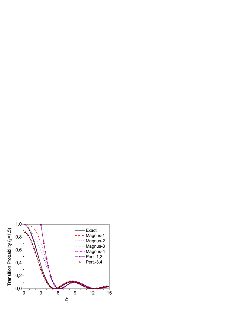
Figure 3: Rectangular step: Transition probabilities as a function of $\xi$, with $\gamma=1.5$. The solid line corresponds to the exact result (196). Broken lines stand for approximations obtained via ME and lines with symbols correspond to perturbation theory, according to the legend. Computations up to fourth order, in the Interaction Picture.

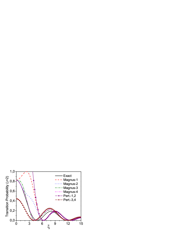
Figure 4: Rectangular step: Transition probabilities as a function of $\xi$, with $\gamma=2$. Lines are coded as in Figure 3. Computations up to fourth order, in the Interaction Picture.

We observe that for the Magnus expansion in the Interaction Picture, the smaller the value of the parameter $\xi$ the better works the approximate solution. As a matter of fact, in the sudden limit, $\xi\ll 1$, ME furnishes the exact result; unlike perturbation theory. As far as the intensity of the perturbation $\gamma$ increases, the quality of the approximations spoils. This effect is much more dramatic for the standard perturbation theory.

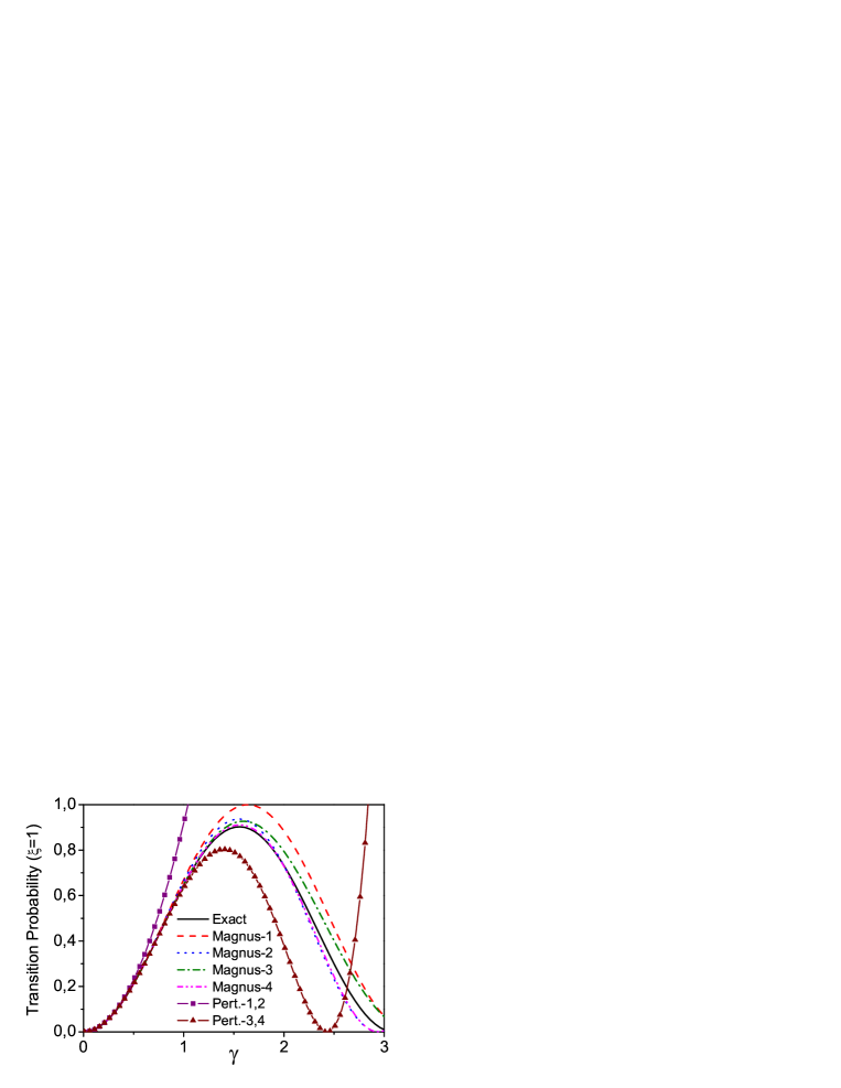
Figure 5: Rectangular step: Transition probabilities as a function of $\gamma$, with $\xi=1$. Lines are coded as in Figure 3. Computations up to fourth order, in the Interaction Picture.

On the other hand, it is clear from (198) that

$$\int_{-\infty}^{t}\|H_{I}(t_{1})\|_{2}\,dt_{1}=\int_{0}^{t}|f(t_{1})|\,dt_{1}=V_{0}\,t,$$

whence $\int_{-\infty}^{t}\|\tilde{H}_{I}(t_{1})\|_{2}\,dt_{1}=\gamma$, and thus Theorem 9 guarantees that the Magnus expansion in the Interaction Picture is convergent if $\gamma<\pi$. Notice that this is always the case for the parameters considered in Figures 3-5. The estimate $\gamma<\pi$ for the convergence domain in the Interaction Picture should be compared with the corresponding one in the Schrödinger picture:

$$\int_{-\infty}^{t}\|\tilde{H}(t_{1})\|_{2}\,dt_{1}=\sqrt{\gamma^{2}+\frac{\xi^{2}}{4}}<\pi.$$

Notice then that, as pointed out in subsection 2.9, a change of picture allows us to improve the convergence of the Magnus expansion.

2- Hyperbolic secant step: Rosen–Zener model. In the Rosen–Zener Hamiltonian [204] the interaction $C(t)$ in (189) is given by the real function $V(t)=V_{0}\,{\rm sech}(t/T)$, where $T$ determines the time-scale. We will use the notation $\gamma=\pi V_{0}T/\hbar$ and $\xi=\omega T=2ET/\hbar$.

The corresponding Hamiltonian in terms of Pauli matrices is

$$H(t)=E\sigma_{3}+V(t)\sigma_{1}\equiv\boldsymbol{a}(t)\cdot\boldsymbol{\sigma},\qquad V(t)=V_{0}/\cosh(t/T),$$ (202)

with $\boldsymbol{a}\equiv(V(t),0,E)$. In the Interaction Picture one has

$$H_{I}(s)=V(s)(\sigma_{1}\cos(\xi s)-\sigma_{2}\sin(\xi s))$$ (203)

in terms of the dimensionless time-variable $s=t/T$. Notice that $\xi$ measures the ratio between the interaction time $T$ and the internal time of the system $\hbar/2E$. From (203), and after straightforward calculation, the first and second ME operators are readily obtained.

The exact result for the transition probability (provided the time interval extends from $-\infty$ to $+\infty$), as well as perturbation theory and Magnus expansion up to second order read [195]

$$P_{ex} = \frac{\sin^{2}\gamma}{\cosh^{2}(\pi\xi/2)}$$

$$P_{pt}^{(1)} = P_{pt}^{(2)}=\frac{\gamma^{2}}{\cosh^{2}(\pi\xi/2)}$$

$$P_{M}^{(1)} = \sin^{2}[\gamma/\cosh(\pi\xi/2)]$$

$$P_{M}^{(2)} = \frac{\sin^{2}\lambda}{\lambda^{2}}\frac{\gamma^{2}}{\cosh^{2}(\pi\xi/2)}$$ (204)

$$\lambda = \gamma\left[\frac{1}{\cosh^{2}(\pi\xi/2)}+\frac{\gamma^{2}g^{2}(\xi)}{\pi^{4}}\right]^{1/2},\quad g(\xi)=8\xi\sum_{k=0}^{\infty}\frac{2k+1}{[(2k+1)^{2}+\xi^{2}]^{2}}.$$

In Figures 6 and 7 we plot some results from the formulae in (4.1.2). In Figure 6 we take $\gamma=1.5$ and in Figure 7 we set $\xi=0.3$.

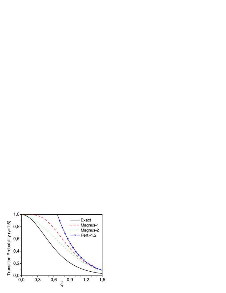
Figure 6: Rosen–Zener model: Transition probabilities (4.1.2) as a function of $\xi$, with $\gamma=1.5$. The solid line stand for the exact result. Broken lines stand for approximations obtained via ME and triangles correspond to perturbation theory, according to the legend. Computations up to second order, in the Interaction Picture.

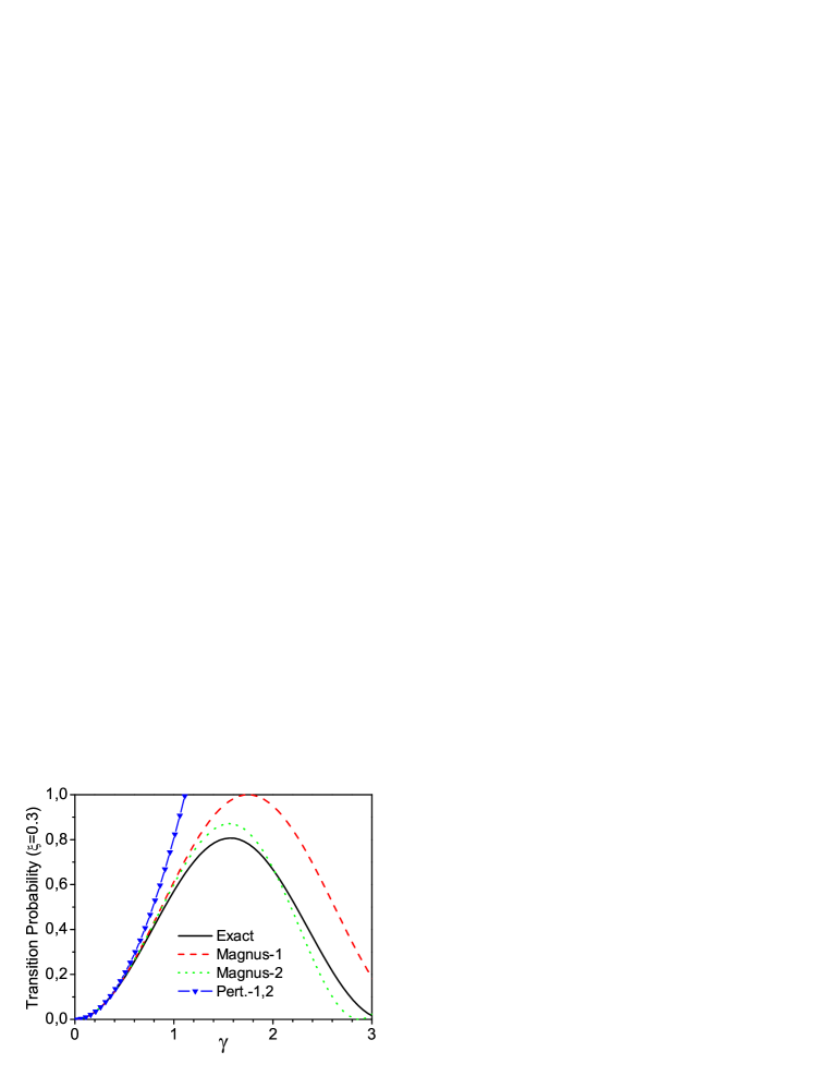
Figure 7: Rosen–Zener model: Transition probabilities as a function of $\gamma$, with $\xi=0.3$. Lines are coded as in Figure 6. Computations up to second order, in the Interaction Picture.

Similarly to the case of the rectangular step, we observe in Figure 6 that the Magnus expansion works better in the sudden regime defined by $\xi\ll 1$, namely, when the internal time of the system $\hbar/2E$ is much larger than the time scale $T$ of the perturbation. Also, Figure 7 illustrates how the approximations spoil as far as the intensity $\gamma$ increases. Notice in both figures the unitarity violation of the approximation built with the usual perturbation theory.

In this case a simple calculation shows that

$$\int_{-\infty}^{\infty}\|\tilde{H}_{I}(t)\|_{2}\,dt=(1/\hbar)\,\int_{\infty}^{\infty}|V(t)|\,dt=V_{0}\pi T/\hbar=\gamma,$$

and thus the Magnus series converges at least for $\gamma<\pi$.

4.2 ME in the Adiabatic Picture

Here we will illustrate the effect of using the Adiabatic Picture introduced in Section 2.9. The use of this type of preliminary transformation is convenient whenever the time scale of the interaction is much larger than the proper time of the unperturbed system.

Since an adiabatic regime conveys a smooth profile for the perturbation, namely, existence of derivatives, the case of the rectangular step cannot be properly used for the sake of illustration.

4.2.1 Linearly forced harmonic oscillator

For the linearly driven harmonic oscillator the procedure yields the exact solution, as in the preceding subsection 4.1.2, albeit the method is a bit more involved technically [140].

4.2.2 Rosen–Zener model

Following [138] we will deal with the Rosen–Zener model (see Section 4.1.2 and [195]) since it allows a clear illustration of the adiabatic regime.

The preliminary linear transformation $G(s)$ defined in (94) for the Hamiltonian (202) is given by $G(s)=\boldsymbol{\hat{b}}\cdot\boldsymbol{\sigma}$, where the unit vector $\boldsymbol{\hat{b}}$ points in the direction $\boldsymbol{b}=\boldsymbol{\hat{a}}+\boldsymbol{\hat{k}}$ ($\boldsymbol{\hat{k}}=$unit vector along the $z$-axis). Remind that $s=t/T$ is the dimensionless time-variable. The evolution operator gets then factorized as

$$U_{G}(s)=G^{\dagger}(s)U(s)G(s_{0}),$$ (205)

which according to (90), satisfies the equation

$$\frac{dU_{G}}{ds}=\tilde{H}_{G}(s)U_{G}.$$ (206)

Here $\tilde{H}_{G}\equiv-iH_{G}/\hbar$ is given by

$$\tilde{H}_{G}(s)=\frac{T}{i\hbar}a\sigma_{3}-i\frac{\theta^{\prime}}{2}\sigma_{2},$$ (207)

with $a^{2}=E^{2}_{0}+V^{2}_{0}/\cosh^{2}s$ and $\cot\theta=(E_{0}/V_{0})\cosh s$.

Next, in analogy to (203), we introduce the Adiabatic Interaction Picture which allows us to integrate the diagonal piece of $\tilde{H}_{G}(s)$. The time-evolution operator gets eventually factorized as

$$U_{G}(s)=\exp\left((-iT/\hbar)\int^{\infty}_{0}\textrm{d}s^{\prime}\,a(s^{\prime})\sigma_{3}\right)U_{G}^{(I)}(s)\exp\left((-iT/\hbar)\int_{-\infty}^{0}\textrm{d}s^{\prime}\,a(s^{\prime})\sigma_{3}\right),$$ (208)

where $U_{G}^{(I)}(s)$ obeys the equation

$$\frac{dU_{G}^{(I)}}{ds}=\tilde{H}_{G}^{(I)}(s)\,U_{G}^{(I)},$$ (209)

with

$$\tilde{H}_{G}^{(I)}(s)=-i(\theta^{\prime}/2)[\sigma_{1}\sin A(s)+\sigma_{2}\cos A(s)],$$ (210)

and

$$A(s)=\frac{2T}{\hbar}\int_{0}^{s}\textrm{d}s^{\prime}\,a(s^{\prime})=\frac{\xi}{2}\ln\frac{1+\rho}{1-\rho}+\frac{2\gamma}{\pi}\arctan\frac{2\gamma}{\pi\xi}\rho.$$ (211)

We have introduced the definition

$$\rho=\{1-[1+(\pi\xi/2\gamma)]\sin^{2}\theta\}^{1/2},$$ (212)

in terms of the dimensionless strength parameter $\gamma=\pi V_{0}T/\hbar$ and $\theta$. Using the ME to first order in the adiabatic basis (which coincides with the fixed one at $s=\pm\infty$) one finds the spin-flip approximate (first order) transition probability

$$^{ad}P_{M}^{(1)}=\sin^{2}\left[\int_{0}^{\theta_{0}}\textrm{d}\theta\sin A(s(\theta))\right].$$ (213)

In Figure 8 we compare the numerical results given by the new approximation (213) with the exact formula $P_{ex}$ in (4.1.2). For the sake of illustration we plot also the results in the usual Interaction Picture to first order in ME (see $P_{M}^{(1)}$ in (4.1.2)). It is noteworthy the gain achieved when using the adiabatic ME in the intermediate regime, namely, moderate values of $\xi$, although only the first order is considered. Here the adiabatic regime corresponds to large values of $\xi=2ET/\hbar$ ($\varepsilon=1/T\ll 1$).

It should be also noticed that for the Hamiltonian (210) one has

$$\int_{s_{0}}^{s}\|\tilde{H}_{G}^{(I)}(s_{1})\|_{2}\,ds_{1}=\frac{1}{2}|\theta(s)-\theta(s_{0})|<\frac{1}{2}2\pi=\pi$$

and thus the convergence condition given by Theorem 9 is always satisfied. In other words, for this example the Magnus expansion is always convergent in the Adiabatic Interaction Picture.

More involved illustrative examples of ME in the Adiabatic Picture may be found in [139, 140].

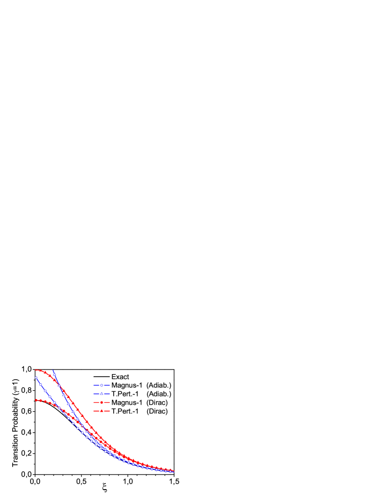
Figure 8: Rosen–Zener model: Transition probability as a function of $\xi$, with $\gamma=1$. The solid line stands for the exact result in (4.1.2). The remaining lines stand for first order computations with ME (circles) and perturbation theory (triangles). Open symbols are for the Adiabatic Picture and solid symbols for the Interaction Picture.

4.3 Fer and Wilcox infinite-product expansions

Next we illustrate the use of Fer and Wilcox infinite-product expansions by using the same time-dependent systems as before.

4.3.1 Linearly forced harmonic oscillator

Since the commutator $[a_{-},a_{+}]$ is a $c$-number, Fer iterated Hamiltonians $H^{(n)}$ with $n>1$ eventually vanish so that $F_{n}=0$ for $n>2$. The Wilcox operators $W_{n}$ with $n>2$ in eq.(106) vanish for the same reason. Thus, in this particular case, the second-order approximation in either method leads to the exact solution of the Schrödinger equation just as ME did. To sum up, the final result reads

$$U_{I}=\e^{\Omega_{1}+\Omega_{2}}=\e^{W_{1}}\e^{W_{2}}=\e^{F_{1}}\e^{F_{2}}=\e^{-i\beta}\e^{-i(\alpha a_{+}+\alpha^{*}a_{-})}\,,$$ (214)

where $\alpha(t)$ and $\beta(t)$ are given in (185) and (186), respectively.

4.3.2 Two-level quantum system: Rectangular step

For the Hamiltonian (194), the first-order Fer and Wilcox operators in the Interaction Picture verify

$$F_{1}=W_{1}=\Omega_{1}=\int_{0}^{t}{\rm d}t_{1}\tilde{H}_{I}(t_{1}),$$ (215)

where $\tilde{H}_{I}(t)$ is given by (198). The explicit expression is collected in (4.1.2) (first equation). Analogously, the second equation there also corresponds to the second-order Wilcox operator $W_{2}=\Omega_{2}$.

To proceed further with Fer’s method we must calculate the modified Hamiltonian $\tilde{H}^{(1)}$ in (96). After straightforward algebra one eventually obtains

$$\tilde{H}^{(1)}=\frac{1}{2\theta}\left(\frac{\sin^{2}\theta}{\theta}-\sin 2\theta+\frac{1}{\theta}\left(\frac{\sin 2\theta}{2\theta}-\cos 2\theta\right)F_{1}\right)\,[F_{1},\tilde{H}_{I}]\;,$$ (216)

where $\theta=(2\gamma/\xi)\sin(\xi/2)$ (notice that $\tilde{H}^{(1)}$ and therefore $F_{2}$ depend on $\sigma_{1}$ and $\sigma_{2}$, while $W_{2}$ is proportional to $\sigma_{3}$). Since it does not seem possible to derive an analytical expression for $F_{2}$, the corresponding matrix elements have been computed by replacing the integral by a conveniently chosen quadrature.

The transition probability $P(t)$ from an initial state with spin up to a state with spin down (or viceversa) is given by (193). This expression has been computed on assuming: $U_{I}\simeq\e^{F_{1}}=\e^{W_{1}}$, $U_{I}\simeq\e^{F_{1}}\e^{F_{2}}$, $U_{I}\simeq\e^{W_{1}}\e^{W_{2}}$, $U_{I}\simeq\e^{F_{1}}\e^{F_{2}}\e^{F_{3}}$ and $U_{I}\simeq\e^{W_{1}}\e^{W_{2}}\e^{W_{3}}$, and the results have been compared with the exact analytical solution (196).

In Figures 9 and 10 we show the transition probability $P$ as a function of $\xi$ for two different values of $\gamma$ ($\gamma=1.5$ and $\gamma=2$, respectively), while in Figure 11 we have plotted $P$ versus $\gamma$ for $\xi$ fixed. Notice that the second order in the Wilcox expansion does not contribute to the transition probability (this is similar to what happens in perturbation theory). On the other hand, Fer’s second-order approximation is already in remarkable agreement with the exact result whereas the third order cannot even be distinguished from the exact result in Figure 10 at the cost of a much larger computational effort. Wilcox approximants preserve unitarity but do not give acceptable approximations.

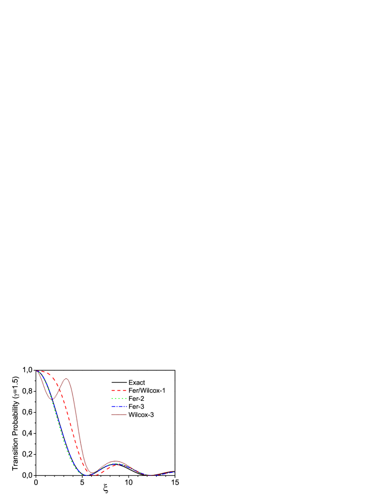
Figure 9: Rectangular step: Transition probability as a function of $\xi$, with $\gamma=1.5$. The solid line corresponds to the exact result (196). Broken lines stand for Fer and Wilcox approximations up to third order. Computations up to third order, in the Interaction Picture.

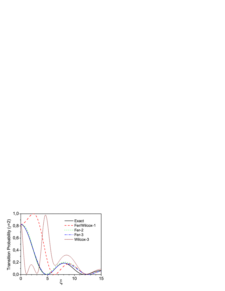
Figure 10: Rectangular step: Transition probability as a function of $\xi$, with $\gamma=2$. Lines are coded as in Figure 9. Computations up to third order, in the Interaction Picture.

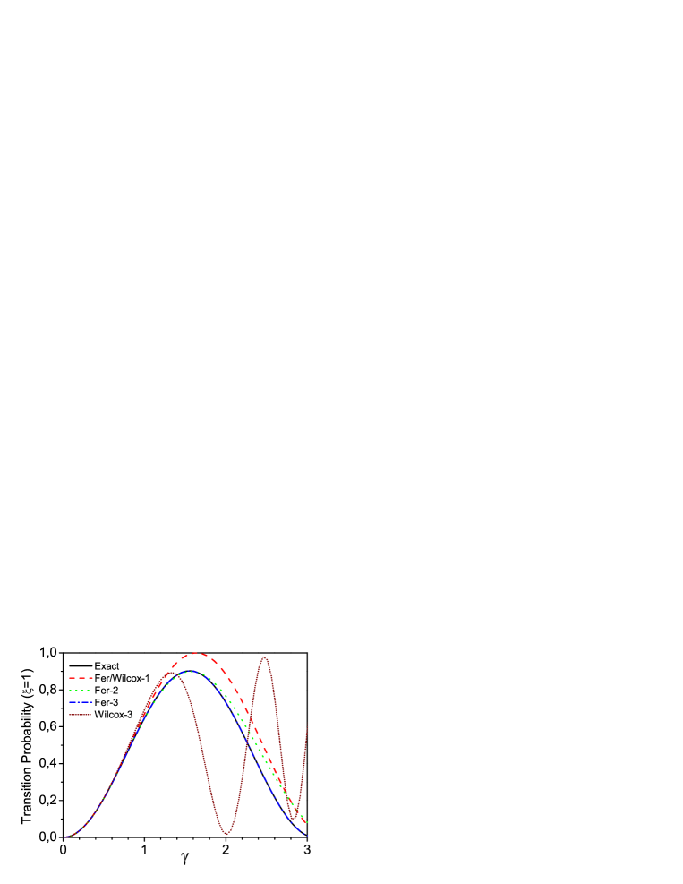
Figure 11: Rectangular step: Transition probability as a function of $\gamma$, with $\xi=1$. Lines are coded as in Figure 9. Computations up to third order, in the Interaction Picture.

4.4 Voslamber iterative method

Just to keep the same structure as in preceding subsections, we mention that the Voslamber iterative method of subsection 3.1 also yields the exact solution for the linearly driven harmonic oscillator after computing the second iteration.

Next, for the two-level system with a rectangular step described by the Hamiltonian (194) we compute the second iterate $\Omega^{(2)}$ and compare with second order ME approximation for $U_{I}$. As a test, we shall obtain again the transition probability $P(t)$ given by (196). The expression (193) will be calculated here on assuming: $U_{I}\simeq\exp{\Omega^{(1)}}=\exp\Omega_{1}$, $U_{I}\simeq\exp({\Omega_{1}+\Omega_{2}})$ and $U_{I}\simeq\exp{\Omega^{(2)}}$.

The second order Magnus approximation to the transition probability is given by (4.1.2), whereas the second iterate is obtained from (3.1),

$$\Omega^{(2)}(t) = -i\frac{\gamma}{\omega}\int_{0}^{\omega t}\{[\sin^{2}(\Delta)+\cos^{2}(\Delta)\cos{\xi}]\,\sigma_{1}$$ (217)

$$+\cos^{2}(\Delta)\sin{\xi}\,\sigma_{2}-\sin(2\Delta)\sin(\xi/2)\,\sigma_{3}\}{\rm d}\xi,$$

where $\Delta\equiv\frac{\gamma}{\omega}|\sin(\xi/2)|$, $\gamma=V_{0}t/\hbar$, $\xi=\omega t$. Since it does not seem possible to derive an analytical expression for $\Omega^{(2)}$, the corresponding matrix elements have been computed by approximating the integral in (217) with a sufficiently accurate quadrature.

In Figure 12, the various approximated transition probabilities as well as the exact result (196) have been plotted as a function of $\xi$ for a fixed value $\gamma=1.5$. We observe that the approximation from the second iterate keeps the trend of the exact solution in a better way that the second order Magnus approximation does.

In Figure 13 we have plotted the corresponding transition probabilities versus $\gamma$ for fixed value $\xi=1$. Although locally the second order Magnus approximation may be more accurate, it seems that the trend of the exact solution is mimicked for a longer interval of $\gamma$.

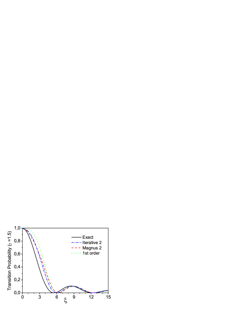
Figure 12: Rectangular step: Transition probability in the two level system as a function of $\xi$, for $\gamma=1.3$: Exact result (4.1.2) (solid line), second iterate of Voslamber method (dashed line), second order ME (dotted line) and first Voslamber iterate (or order in ME) (dash-dotted line). Computations are done in the Interaction Picture.

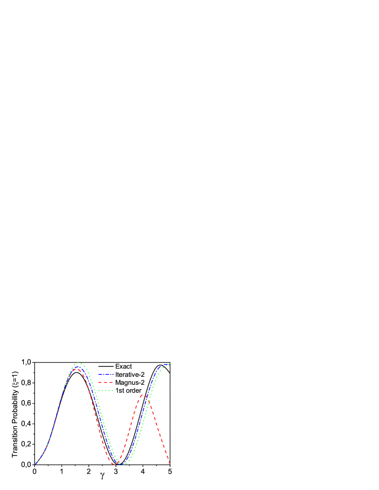
Figure 13: Rectangular step: Transition probability in the two level system as a function of $\gamma$, for $\xi=1$. Lines are coded as in Figure 12. Computations are done in the Interaction Picture.

As it has already been pointed out above, the Magnus expansion works the better the more sudden the perturbation. Thus, the re-summation involved in the iterative method improves a bit that issue. Further results on the present example may be found in [193].

4.5 Linear periodic systems: Floquet–Magnus formalism

Next we deal with a periodically driven harmonic oscillator, where the infinite expansions obtained from Floquet–Magnus recurrences (see subsection 3.2), are utterly summed. Comparison with the exact solution illustrates the feasibility of the method.

The particular system we consider is described by the Hamiltonian (179) with $f(t)=\frac{\beta}{\sqrt{2}}\cos\omega t$ and $\omega_{0}<\omega$. Once the recurrences of the Floquet–Magnus expansion (see section 3.2) are explicitly computed for several orders, their general term may be guessed by inspection. For the Floquet operator we get

$$F=-i\left[\frac{\omega_{0}}{2}\left(p^{2}+q^{2}\right)-\beta\frac{\omega_{0}}{\omega}\sum_{k=0}^{\infty}\left(\frac{\omega_{0}}{\omega}\right)^{k}q+\beta^{2}\frac{\omega_{0}}{4\omega^{2}}\sum_{k=0}^{\infty}\left(2k+1\right)\left(\frac{\omega_{0}}{\omega}\right)^{k}\right],$$ (218)

and the associated transformation results from

$$\Lambda(t) = i\beta^{2}\frac{\omega_{0}}{\omega^{3}}\left[\sin\left(\omega t\right)\sum\limits_{k=0}^{\infty}\left(k+1\right)\left(\frac{\omega_{0}}{\omega}\right)^{k}-\frac{\omega t}{2}\sum\limits_{k=0}^{\infty}\left(\frac{\omega_{0}}{\omega}\right)^{k}\right]-$$ (219)

$$i\left[\sin\left(\omega t\right)q+\omega_{0}\left(\cos\left(\omega t\right)-1\right)p\right]\frac{\beta}{\omega}\sum\limits_{k=0}^{\infty}\left(\frac{\omega_{0}}{\omega}\right)^{k}.$$

The resulting series may be summed in closed form thus yielding the Floquet operator

$$F=-i\frac{\omega_{0}}{2}\left[\left(q-\frac{\beta}{\omega_{0}(\rho^{2}-1)}\right)^{2}+p^{2}\right]-i\frac{\beta^{2}}{4\omega_{0}\left(\rho^{2}-1\right)},$$ (220)

with $\rho\equiv\omega/\omega_{0}$. Its eigenvalues are the so-called Floquet eigenenergies [144]

$$E_{n}=\omega_{0}\left(n+\frac{1}{2}\right)+\frac{\beta^{2}}{4\omega_{0}\left(\rho^{2}-1\right)}.$$ (221)

The corresponding $\Lambda$ transformation after summation of the series in (219) is

$$\Lambda(t)=i\frac{\beta/\omega_{0}}{1-\rho^{2}}\left[\left(\rho\sin\omega t\right)q+(\cos\omega t-1)p+\left(\frac{2\rho^{2}}{1-\rho^{2}}+\cos\omega t\right)\frac{\beta\sin\omega t}{4\omega}\right].$$ (222)

Notice that, as they should, both operators are skew-Hermitian and reproduce the exact solution of the problem.

5 Numerical integration methods based on the Magnus expansion

5.1 Introduction

The Magnus expansion as formulated in section 2 has found extensive use in mathematical physics, quantum chemistry, control theory, etc, essentially as a perturbative tool in the treatment of the linear equation

$$Y^{\prime}=A(t)Y,\qquad Y(t_{0})=Y_{0}.$$ (223)

When the recurrence (49)-(50) is applied, one is able to get explicitly the successive terms $\Omega_{k}$ in the series defining $\Omega$ as linear combinations of multivariate integrals containing commutators acting iteratively on the coefficient matrix $A$, as in (42)-(4). As a result, with this scheme analytical approximations to the exact solution are constructed explicitly. These approximate solutions are fairly accurate inside the convergence domain, especially when high order terms in the Magnus series are taken into account, as illustrated by the examples considered in section 4.

There are several drawbacks, however, involved in the procedure developed so far, especially when one tries to find accurate approximations to the solution for very long times. The first one is implicitly contained in the analysis done in section 2: the size of the convergence domain of the Magnus series may be relatively small. The logarithm of the exact solution $Y(t)$ may have complex singularities and this implies that no series expansion can converge beyond the first singularity. This disadvantage may be up to some point avoided by using different pictures, e.g. the transformations shown in section 2.9, in order to increase the convergence domain of the Magnus expansion, a fact also illustrated by several examples in section 4. Unfortunately, these preliminary transformations sometimes either do not guarantee convergence or the rate of convergence of the series is very slow. In that case, accurate results can only be obtained provided a large number of terms in the series are taken into account.

The second drawback is the increasingly complex structure of the terms $\Omega_{k}$ in the Magnus series: each $\Omega_{k}$ is a $k$-multivariate integral involving a linear combination of $(k-1)$-nested commutators of $A$ evaluated at different times $t_{i}$, $i=1,\ldots,k$. Although in some cases these expressions can be computed explicitly (for instance, when the elements of $A$ and its commutators are polynomial or trigonometric functions), in general a special procedure has to be designed to approximate multivariate integrals and reduce the number of commutators involved.

When the entries of the coefficient matrix $A(t)$ are complicated functions of time or they are only known for certain values of $t$, numerical approximation schemes are unavoidable. In many cases it is thus desirable to obtain just numerical approximations to the exact solution at many different times. This section is devoted precisely to the Magnus series expansion as a tool to build numerical integrators for equation (223).

Before embarking ourselves in exposing the technical details contained in this construction, let us first introduce several concepts which are commonplace in the context of the numerical integration of differential equations.

Given the general (nonlinear) ordinary differential equation (ODE)

$${\bf x}^{\prime}={\bf f}(t,{\bf x}),\qquad\qquad{\bf x}(t_{0})={\bf x}_{0}\in\mathbb{C}^{d},$$ (224)

standard numerical integrators, such as Runge–Kutta and multistep methods, proceed as follows. First the whole time interval $[t_{0},t_{f}]$, is split into $N$ subintervals, $[t_{n-1},t_{n}],\ n=1,\ldots,N$, with $t_{N}=t_{f}$, and subsequently the value of ${\bf x}(t_{n})$ is approximated with a time-stepping advance procedure of the form

$$\mathbf{x}_{n+1}=\Phi(h_{n},\mathbf{x}_{n},\ldots,h_{0},\mathbf{x}_{0})$$ (225)

starting from $\mathbf{x}_{0}$. Here the map $\Phi$ depends on the specific numerical method and $h_{n}=t_{n+1}-t_{n}$ are the time steps. For simplicity in the presentation we consider a constant time step $h$, so that $t_{n}=t_{0}+n\,h$. In this way one gets ${\bf x}_{n+1}$ as an approximation to ${\bf x}(t_{n+1})$. In other words, the exact evolution of the system (224) is replaced by the discrete or numerical flow (225). The simplest of all numerical methods for (224) is the explicit Euler scheme

$$\mathbf{x}_{n+1}=\mathbf{x}_{n}+h\,{\bf f}(t_{n},{\bf x}_{n}).$$ (226)

It computes approximations $\mathbf{x}_{n}$ to the values $\mathbf{x}(t_{n})$ of the solution using one explicit evaluation of $\mathbf{f}$ at the already computed value $\mathbf{x}_{n-1}$. In general, the numerical method (225) is said to be of order $p$ if, assuming ${\bf x}_{n}={\bf x}(t_{n})$, then ${\bf x}_{n+1}={\bf x}(t_{n+1})+\mathcal{O}(h^{p+1})$. Thus, in particular, Euler method is of order one.

Of course, more elaborate and efficient general purpose algorithms, using several $\mathbf{f}$ evaluations per step, have been proposed along the years for the numerical treatment of equation (224). In fact, any standard software package and program library contains dozens of routines aimed to provide numerical approximations with several degrees of accuracy, including (explicit and implicit) Runge–Kutta methods, linear multistep methods, extrapolation schemes, etc, with fixed or adaptive step size. They are designed in such a way that the user has to provide only the initial condition and the function $\mathbf{f}$ to obtain approximations at any given time.

This being the case, one could ask the following question: if general purpose integrators are widely available for the integration of the linear equation (223) (which is a particular case of (224)), what is the point in designing new and somehow sophisticated algorithms for this specific problem?

It turns out that in the same way as for classical time-dependent perturbation theory, the qualitative properties of the exact solution are not preserved by the numerical approximations obtained by standard integrators. This motivates the study of the Magnus expansion with the ultimate goal of constructing numerical integration methods. We will show that highly accurate schemes can be indeed designed, which in addition preserve qualitative properties of the system. The procedure can also incorporate the tools developed for the analytical treatment, such as preliminary linear transformations, to end up with improved numerical algorithms.

We first summarize the main features of the well know class of Runge–Kutta methods as representative of integrators of the form (225). They are introduced for the general nonlinear ODE (224) and subsequently adapted to the linear case (223).

5.2 Runge–Kutta methods

The Runge–Kutta (RK) class of methods are possibly the most frequently used algorithms for numerically solving ODEs. Among them, perhaps the most successful during more than half a century has been the 4th-order method, which applied to equation (224) provides the following numerical approximation for the integration step $t_{n}\mapsto t_{n+1}=t_{n}+h$:

$${\bf Y}_{1} = {\bf x}_{n}$$

$${\bf Y}_{2} = {\bf x}_{n}+\frac{h}{2}{\bf f}(t_{n},{\bf Y}_{1})$$

$${\bf Y}_{3} = {\bf x}_{n}+\frac{h}{2}{\bf f}(t_{n}+\frac{h}{2},{\bf Y}_{2})$$ (227)

$${\bf Y}_{4} = {\bf x}_{n}+h{\bf f}(t_{n}+\frac{h}{2},{\bf Y}_{3})$$

$${\bf x}_{n+1} = {\bf x}_{n}+\frac{h}{6}\left({\bf f}(t_{n},{\bf Y}_{1})+2{\bf f}(t_{n}+\frac{h}{2},{\bf Y}_{2})+2{\bf f}(t_{n}+\frac{h}{2},{\bf Y}_{3})+{\bf f}(t_{n}+h,{\bf Y}_{4})\right).$$

Notice that the function ${\bf f}$ can always be computed explicitly because each ${\bf Y}_{i}$ depends only on the ${\bf Y}_{j},\ j<i$, previously evaluated. To measure the computational cost of the method, it is usual to consider that the evaluation of the function ${\bf f}(t,{\bf x})$ is the most consuming part. In this sense, scheme (5.2) requires four evaluations, which is precisely the number of stages (or inner steps) in the algorithm.

The general class of $s$-stage Runge–Kutta methods are characterized by the real numbers $a_{ij}$, $b_{i}$ ($i,j=1,\ldots,s$) and $c_{i}=\sum_{j=1}^{s}a_{ij}$, as

$${\bf Y}_{i} = {\bf x}_{n}+h\sum_{j=1}^{s}a_{ij}\,{\bf f}(t_{n}+c_{j}h,{\bf Y}_{j}),\qquad i=1,\ldots,s$$

$${\bf x}_{n+1} = {\bf x}_{n}+h\sum_{i=1}^{s}b_{i}\,{\bf f}(t_{n}+c_{i}h,{\bf Y}_{i}),$$ (228)

where ${\bf Y}_{i}$, $i=1,\ldots,s$ are the intermediate stages. For simplicity, the associated coefficients are usually displayed with the so-called Butcher tableau [37, 100] as follows:

$$\begin{array}[]{c|ccccc}c_{1}&a_{11}&&\ldots&&a_{1s}\\ \vdots&\vdots&&&&\vdots\\ c_{s}&a_{s1}&&\ldots&&a_{ss}\\ \hline\cr&b_{1}&&\ldots&&b_{s}\end{array}$$ (229)

If $a_{ij}=0$, $j\geq i$, then the intermediate stages ${\bf Y}_{i}$ can be evaluated recursively and the method is explicit. In that case the zero $a_{ij}$ coefficients (in the upper triangular part of the tableau) are omitted for clarity. With this notation, ‘the’ 4th-order Runge–Kutta method (5.2) can be expressed as

$$\begin{array}[]{c|cccc}0&&&&\\ \frac{1}{2}&\frac{1}{2}&&&\\ \frac{1}{2}&0&\frac{1}{2}&&\\ 1&0&0&1&\\ \hline\cr&\ \frac{1}{6}&\ \frac{2}{6}&\ \frac{2}{6}&\ \frac{1}{6}\end{array}$$ (230)

Otherwise, the scheme is implicit and requires to numerically solve a system of $s\,d$ nonlinear equations of the form

$${\bf y}={\bf X}_{n}+h\,{\bf G}(h,{\bf y}),$$ (231)

where ${\bf y}=({\bf Y}_{1},\ldots,{\bf Y}_{s})^{T},{\bf X}_{n}=({\bf x}_{n},\ldots,{\bf x}_{n})^{T}\in\mathbb{R}^{sd}$, and ${\bf G}$ is a function which depends on the method. A standard procedure to get $\mathbf{x}_{n+1}$ from (231) is applying simple iteration:

$${\bf y}^{[j]}={\bf X}_{n}+h\,{\bf G}(h,{\bf y}^{[j-1]}),\qquad j=1,2,\ldots$$ (232)

When $h$ is sufficiently small, the iteration starts with ${\bf y}^{[0]}={\bf X}_{n}$ and stops once $\|{\bf y}^{[j]}-{\bf y}^{[j-1]}\|$ is smaller than a prefixed tolerance. Of course, more sophisticated techniques can be used [100].

After these general considerations, let us turn our attention now to the linear equation (223). When dealing with numerical methods applied to this equation, it is important to keep in mind that the relevant small parameter here is no longer the norm of the matrix $A(t)$ as in the analytical treatment, but the time step $h$. For this reason, the concept of order of accuracy of a method is different in this context. Now ${\bf f}(t,{\bf x})=A(t){\bf x}$ and the general class of $s$-stage Runge–Kutta methods adopt the more compact form

$${\bf Y}_{i} = {\bf x}_{n}+h\sum_{j=1}^{s}a_{ij}A_{j}{\bf Y}_{j},\qquad i=1,\ldots,s$$

$${\bf x}_{n+1} = {\bf x}_{n}+h\sum_{i=1}^{s}b_{i}A_{i}{\bf Y}_{i},$$ (233)

with $A_{i}=A(t_{n}+c_{i}h)$. In terms of matrices, this is equivalent to

$$\left\{\begin{array}[]{c}{\bf Y}_{1}\\ \vdots\\ {\bf Y}_{s}\end{array}\right\} = \left\{\begin{array}[]{c}{\bf x}_{n}\\ \vdots\\ {\bf x}_{n}\end{array}\right\}+h\widetilde{A}\left\{\begin{array}[]{c}{\bf Y}_{1}\\ \vdots\\ {\bf Y}_{s}\end{array}\right\},\qquad\mbox{with}\qquad\widetilde{A}=\left(\begin{array}[]{ccc}a_{11}A_{1}&\cdots&a_{1s}A_{s}\\ \vdots&&\vdots\\ a_{s1}A_{1}&\cdots&a_{ss}A_{s}\end{array}\right)$$ (246)

$${\bf x}_{n+1} = {\bf x}_{n}+h\left(\begin{array}[]{ccc}b_{1}A_{1}&\cdots&\ b_{s}A_{s}\end{array}\right)\left\{\begin{array}[]{c}{\bf Y}_{1}\\ \vdots\\ {\bf Y}_{s}\end{array}\right\},$$ (251)

so that the application of the method for the integration step $t_{n}\mapsto t_{n+1}=t_{n}+h$ can also be written as

$${\bf x}_{n+1}=\left(I_{d}+h\left(\begin{array}[]{ccc}b_{1}A_{1}&\cdots&b_{s}A_{s}\end{array}\right)\left(I_{sd}-h\widetilde{A}\right)^{-1}\mathbb{I}_{sd\times d}\right){\bf x}_{n},$$ (252)

where $\mathbb{I}_{sd\times d}=(I_{d},I_{d},\ldots,I_{d})^{T}$ and $I_{d}$ is the $d\times d$ identity matrix. For instance, taking $s=2$ and using Matlab this can be easily implemented as follows

$$\begin{array}[]{l}A=[a11*A1\ \ \ a12*A2\ ;\ a21*A1\ \ \ a22*A2];\\ x=(Id+h*[b1*A1\ \ \ b2*A2]*((I2d-h*A)\backslash[Id\ \ \ Id]^{\prime}))*x;\end{array}$$

where $b1,b2,a11,\ldots,a22$ are the coefficients of the method, $A1,A2$ correspond to $A_{1},A_{2}$ and $Id$, $I2d$ are the identity matrices of dimension $d$ and $2d$, respectively.

There exists an extensive literature about RK methods built for many different purposes [37, 100]. It is therefore reasonable to look for the most appropriate scheme to be used for each problem. In practice, explicit RK methods are preferred, because its implementation is usually simpler. They typically require more stages than implicit methods and, in general, a higher number of evaluations of the matrix $A(t)$, although this is not always the case. For instance, the 4-stage fourth order method (5.2) only requires two new evaluations of $A(t)$ per step ($A(t_{n}+h/2)$ and $A(t_{n}+h)$), which is precisely the minimum number of evaluations needed by any fourth order method. In our numerical examples we will also use the 7-stage sixth order method with coefficients [37, p. 203-205]

$$\begin{array}[]{c|ccccccc}0&&&&&&&\\ \frac{5-\sqrt{5}}{10}&\frac{5-\sqrt{5}}{10}&&&&&&\\ \frac{5+\sqrt{5}}{10}&\frac{-\sqrt{5}}{10}&\frac{5+2\sqrt{5}}{10}&&&&&\\ \frac{5-\sqrt{5}}{10}&\frac{-15+7\sqrt{5}}{20}&\frac{-1+\sqrt{5}}{4}&\frac{15-7\sqrt{5}}{10}&&&&\\ \frac{5+\sqrt{5}}{10}&\frac{5-\sqrt{5}}{60}&0&\frac{1}{6}&\frac{15+7\sqrt{5}}{60}&&&\\ \frac{5-\sqrt{5}}{10}&\frac{5+\sqrt{5}}{60}&0&\frac{9-5\sqrt{5}}{12}&\frac{1}{6}&\frac{-5+3\sqrt{5}}{10}&&\\ 1&\frac{1}{6}&0&\frac{-55+25\sqrt{5}}{12}&\frac{-25-7\sqrt{5}}{12}&5-2\sqrt{5}&\frac{5+\sqrt{5}}{2}&\\ \hline\cr&\frac{1}{12}&0&0&0&\frac{5}{12}&\frac{5}{12}&\frac{1}{12}\end{array}$$ (253)

Observe that this method only requires three new evaluations of the matrix $A(t)$ per step. This is, in fact, the minimum number for a sixth-order method. Other implicit RK schemes widely used in the literature involving the minimum number of stages at each order are based on Gauss–Legendre collocation points [100]. For instance, the corresponding methods of order four and six (with two and three stages, respectively) have the following coefficients:

$$\begin{array}[]{c|cc}\frac{3-\sqrt{3}}{6}&\frac{1}{4}&\frac{3-2\sqrt{3}}{12}\\ \frac{3+\sqrt{3}}{6}&\frac{3+2\sqrt{3}}{12}&\frac{1}{4}\\ \hline\cr&\frac{1}{2}&\frac{1}{2}\end{array}\qquad\qquad\begin{array}[]{c|ccccc}\frac{5-\sqrt{15}}{10}&\frac{5}{36}&&\frac{2}{9}-\frac{\sqrt{15}}{15}&&\frac{5}{36}-\frac{\sqrt{15}}{30}\\ \frac{1}{2}&\frac{5}{36}+\frac{\sqrt{15}}{24}&&\frac{2}{9}&&\frac{5}{36}+\frac{\sqrt{15}}{24}\\ \frac{5+\sqrt{15}}{10}&\frac{5}{36}+\frac{\sqrt{15}}{30}&&\frac{2}{9}+\frac{\sqrt{15}}{15}&&\frac{5}{36}\\ \hline\cr&\frac{5}{18}&&\frac{4}{9}&&\frac{5}{18}\end{array}$$ (254)

5.3 Preservation of qualitative properties

Notice that the numerical solution provided by the class of Runge–Kutta schemes, and in general by an integrator of the form (225), is constructed as a sum of vectors in $\mathbb{R}^{d}$. Let us point out some (undesirable) consequences of this fact. Suppose, for instance, that $\mathbf{x}$ is a vector known to evolve on a sphere. One does not expect that $\mathbf{x}_{n}$ built as a sum of two vectors as in (225) preserves this feature of the exact solution, whereas approximations of the form $\mathbf{x}_{n+1}=Q_{n}\mathbf{x}_{n}$, with $Q_{n}$ an orthogonal matrix, clearly lie on the sphere.

In section 3.3 we have introduced isospectral flows (143), which include as a particular case the system

$$Y^{\prime}=[A(t),Y],\qquad Y(t_{0})=Y_{0},$$ (255)

with $A$ a skew-symmetric matrix. As we have shown there, if $Y_{0}$ is a symmetric matrix, the exact solution can be factorized as $Y(t)=Q(t)Y_{0}Q^{T}(t)$, with $Q(t)$ an orthogonal matrix satisfying the equation

$$Q^{\prime}=A(t)Q,\qquad Q(0)=I$$ (256)

and, in addition, $Y(t)$ and $Y(0)$ have the same eigenvalues. This is also true when $Y$ is Hermitian, $A$ is skew-Hermitian and $Q$ is unitary, in which case (255) and (256) can be interpreted as particular examples of the Heisenberg and Schrödinger equations in Quantum Mechanics, respectively.

When a numerical scheme of the form (225) is applied to (256), in general, the approximations $Q_{n}$ will no longer be unitary matrices and therefore $Y_{n}$ and $Y_{0}$ will not be unitarily similar. As a result, the isospectral character of the system (255) is lost in the numerical description. Observe that explicit Runge–Kutta methods employ the ansatz that locally the solution of the differential equation behaves like a polynomial in $t$, so that one cannot expect that the approximate solution be a unitary matrix. In this sense, explicit Runge–Kutta methods present the same drawbacks in the numerical analysis of differential equations as the standard time-dependent perturbation theory when looking for analytical approximations.

Implicit Runge–Kutta methods, on the other hand, can be considered as rational approximations, and in some cases the outcome they provide is a unitary matrix. For this class of methods, however, matrices of relatively large sizes have to be inverted, making the algorithms computationally expensive. Furthermore, the evolution of many systems (including highly oscillatory problems) can not be efficiently approximated neither by polynomial nor rational approximations.

With all these considerations in mind, a pair of questions arise in a quite natural way:

• Is it possible to design numerical integration methods for equation (224) such that the corresponding numerical approximations still preserve the main qualitative features of the exact solution?

• Since the Magnus expansion constitutes an extremely useful procedure for obtaining analytical (as opposed to numerical) approximate solutions to the linear evolution equation (223), is it feasible to construct efficient numerical integration schemes from the general formulation exposed in section 2?

It turns out that both questions can be answered in the affirmative. As a matter of fact, it has been trying to address (Q1) how the field of geometric numerical integration has been developed during the last years. Here the aim is to reproduce the qualitative features of the solution of the differential equation which is being discretised, in particular its geometric properties. The motivation for developing such structure-preserving algorithms arises independently in areas of research as diverse as celestial mechanics, molecular dynamics, control theory, particle accelerators physics, and numerical analysis [99, 119, 146, 165, 166].

Although diverse, the systems appearing in these areas have one important common feature. They all preserve some underlying geometric structure which influences the qualitative nature of the phenomena they produce. In the field of geometric numerical integration these properties are built into the numerical method, which gives the method an improved qualitative behaviour, but also allows for a significantly more accurate long-time integration than with general-purpose methods.

In addition to the construction of new numerical algorithms, an important aspect of geometric integration is the explanation of the relationship between preservation of the geometric properties of a numerical method and the observed favourable error propagation in long-time integration.

Geometric numerical integration has been an active and interdisciplinary research area during the last decade, and nowadays is the subject of intensive development. Perhaps the most familiar examples of geometric integrators are symplectic integration algorithms in classical Hamiltonian dynamics, symmetric integrators for reversible systems and methods preserving first integrals and numerical methods on manifolds [99].

A particular class of geometric numerical integrators are the so-called Lie-group methods. If the matrix $A(t)$ in (223) belongs to a Lie algebra $\mathfrak{g}$, the aim of Lie-group methods is to construct numerical solutions staying in the corresponding Lie group $\mathcal{G}$ [119].

With respect to question (Q2) above, it will be the subject of the next subsection, where the main issues involved in the construction of numerical integrators based on the Magnus expansion are analyzed. The methods thus obtained preserve the qualitative properties of the system and in addition are highly competitive with other more conventional numerical schemes with respect to accuracy and computational effort. They constitute, therefore, clear examples of Lie-group methods.

5.4 Magnus integrators for linear systems

Since the Magnus series only converges locally, as we have pointed out before, when the length of the time-integration interval exceeds the bound provided by Theorem 9, and in the spirit of any numerical integration method, the usual procedure consists in dividing the time interval $[t_{0},t_{f}]$ into $N$ steps such that the Magnus series converges in each subinterval $[t_{n-1},t_{n}]$, $n=1,\ldots,N$, with $t_{N}=t_{f}$. In this way the solution of (223) at the final time $t_{f}$ is represented by

$$Y(t_{N})=\prod_{n=1}^{N}\exp(\Omega(t_{n},t_{n-1}))\,Y_{0},$$ (257)

and the series $\Omega(t_{n},t_{n-1})$ has to be appropriately truncated.

Early steps in this approach were taken in [49] and [50], where second and fourth order numerical schemes were used for calculations of collisional inelasticity and potential scattering, respectively. Those authors were well aware that the resulting integration method “would become practical only when the advantage of being able to use bigger step sizes outweighs the disadvantage in having to evaluate the integrals involved in the Magnus series and then doing the exponentiation” [49]. Later on, by following a similar approach, Devries [62] designed a numerical procedure for determining a fourth order approximation to the propagator employed in the integration of the single channel Schrödinger equation, but it was in the pioneering work [120] where Iserles and Nørsett carried out the first systematic study of the Magnus expansion with the aim of constructing numerical integration algorithms for linear problems. To design the new integrators, the explicit time dependency of each term $\Omega_{k}$ had to be analyzed, in particular its order of approximation in time to the exact solution.

Generally speaking, the process of rendering the Magnus expansion a practical numerical integration algorithm involves three steps. First, the $\Omega$ series is truncated at an appropriate order. Second, the multivariate integrals in the truncated series $\Omega^{[p]}=\sum_{i=1}^{p}\Omega_{i}$ are replaced by conveniently chosen approximations. Third, the exponential of the matrix $\Omega^{[p]}$ has to be computed. We now briefly consider the first two issues, whereas the general problem of evaluating the matrix exponential will be treated in section 5.6.

We have shown in subsection 2.6 that the Magnus expansion is time symmetric. As a consequence of eq. (66), if $A(t)$ is analytic and one evaluates its Taylor series centered around the midpoint of a particular subinterval $[t_{n},t_{n}+h]$, then each term in $\Omega_{k}$ is an odd function of $h$, and thus $\Omega_{2s+1}=\mathcal{O}(h^{2s+3})$ for $s\geq 1$. Equivalently, $\Omega^{[2s-2]}=\Omega+\mathcal{O}(h^{2s+1})$ and $\Omega^{[2s-1]}=\Omega+\mathcal{O}(h^{2s+1})$. In other words, for achieving an integration method of order $2s$ ($s>1$) only terms up to $\Omega_{2s-2}$ in the $\Omega$ series are required [22, 120]. For this reason, in general, only even order methods are considered.

Once the series expansion is truncated up to an appropriate order, the multidimensional integrals involved have to be computed or at least conveniently approximated. Although at first glance this seems to be a quite difficult enterprise, it turns out that their very structure allows one to approximate all the multivariate integrals appearing in $\Omega$ just by evaluating $A(t)$ at the nodes of a univariate quadrature [120].

To illustrate how this task can be accomplished, let us expand the matrix $A(t)$ around the midpoint, $t_{1/2}\equiv t_{n}+h/2$, of the subinterval $[t_{n},t_{n+1}]$,

$$A(t)=\sum_{j=0}^{\infty}a_{j}\left(t-t_{1/2}\right)^{j},\qquad\mbox{ where }\quad a_{j}=\frac{1}{j!}\,\frac{d^{j}A(t)}{dt^{j}}\big{|}_{t=t_{1/2}},$$ (258)

and insert the series (258) into the recurrence defining the Magnus expansion (49)-(50). In this way one gets explicitly the expression of $\Omega_{k}$ up to order $h^{6}$ as

$$\Omega_{1} = ha_{0}+h^{3}\frac{1}{12}a_{2}+h^{5}\frac{1}{80}a_{4}+\mathcal{O}(h^{7})$$

$$\Omega_{2} = h^{3}\frac{-1}{12}[a_{0},a_{1}]+h^{5}\Big{(}\frac{-1}{80}[a_{0},a_{3}]+\frac{1}{240}[a_{1},a_{2}]\Big{)}+\mathcal{O}(h^{7})$$

$$\Omega_{3} = h^{5}\Big{(}\frac{1}{360}[a_{0},a_{0},a_{2}]-\frac{1}{240}[a_{1},a_{0},a_{1}]\Big{)}+\mathcal{O}(h^{7})$$ (259)

$$\Omega_{4} = h^{5}\frac{1}{720}[a_{0},a_{0},a_{0},a_{1}]+\mathcal{O}(h^{7}),$$

whereas $\Omega_{5}=\mathcal{O}(h^{7})$, $\Omega_{6}=\mathcal{O}(h^{7})$ and $\Omega_{7}=\mathcal{O}(h^{9})$. Here we write for clarity $[a_{i_{1}},a_{i_{2}},\ldots,a_{i_{l-1}},a_{i_{l}}]\equiv[a_{i_{1}},[a_{i_{2}},[\ldots,[a_{i_{l-1}},a_{i_{l}}]\ldots]]]$. Notice that, as anticipated, only odd powers of $h$ appear in $\Omega_{k}$ and, in particular, $\Omega_{2i+1}=\mathcal{O}(h^{2i+3})$ for $i>1$.

Let us denote $\alpha_{i}\equiv h^{i}a_{i-1}$. Then $[\alpha_{i_{1}},\alpha_{i_{2}},\ldots,\alpha_{i_{l-1}},\alpha_{i_{l}}]$ is an element of order $h^{i_{1}+\cdots+i_{l}}$. In fact, the matrices $\{\alpha_{i}\}_{i\geq 1}$ can be considered as the generators (with grade $i$) of a graded free Lie algebra $\mathcal{L}(\alpha_{1},\alpha_{2},\ldots)$ [182]. It turns out that it is possible to build methods of order $p\equiv 2s$ by considering only terms involving $\alpha_{1},\ldots,\alpha_{s}$ in $\Omega$. Then, these terms can be approximated by appropriate linear combinations of the matrix $A(t)$ evaluated at different points. In particular, up to order four we have to approximate

$$\Omega=\alpha_{1}-\frac{1}{12}[\alpha_{1},\alpha_{2}]+\mathcal{O}(h^{5}),$$ (260)

whereas up to order six the relevant expression is

$$\Omega = \alpha_{1}+\frac{1}{12}\alpha_{3}-\frac{1}{12}[\alpha_{1},\alpha_{2}]+\frac{1}{240}[\alpha_{2},\alpha_{3}]+\frac{1}{360}[\alpha_{1},\alpha_{1},\alpha_{3}]$$

$$-\frac{1}{240}[\alpha_{2},\alpha_{1},\alpha_{2}]+\frac{1}{720}[\alpha_{1},\alpha_{1},\alpha_{1},\alpha_{2}]+\mathcal{O}(h^{7}).$$

In order to present methods which can be easily adapted for different quadrature rules we introduce the averaged (or generalized momentum) matrices

$$A^{(i)}(h)\equiv\frac{1}{h^{i}}\int_{t_{n}}^{t_{n}+h}\,\left(t-t_{1/2}\right)^{i}A(t)dt=\frac{1}{h^{i}}\int_{-h/2}^{h/2}t^{i}A(t+t_{1/2})dt$$ (262)

for $i=0,\ldots,s-1$. If their exact evaluation is not possible or is computationally expensive, a numerical quadrature may be used instead. Suppose that $b_{i}$, $c_{i}$, $(i=1,\ldots,k)$, are the weights and nodes of a particular quadrature rule, say $X$ (we will use $X=G$ for Gauss–Legendre quadratures and $X=NC$ for Newton–Cotes quadratures) of order $p$, respectively [2],

$$A^{(0)}=\int_{t_{n}}^{t_{n}+h}A(t)dt=h\sum_{i=1}^{k}b_{i}A_{i}+\mathcal{O}(h^{p+1}),$$

with $A_{i}\equiv A(t_{n}+c_{i}h)$. Then it is possible to approximate all the integrals $A^{(i)}$ (up to the required order) just by using only the evaluations $A_{i}$ at the nodes $c_{i}$ of the quadrature rule required to compute $A^{(0)}$. Specifically,

$$A^{(i)}=h\sum_{j=1}^{k}b_{j}\left(c_{j}-\frac{1}{2}\right)^{i}A_{j}.\qquad\quad i=0,\ldots,s-1,$$ (263)

or equivalently, $A^{(i)}=h\sum_{j=1}^{k}\left(Q^{(s,k)}_{X}\right)_{ij}A_{j}$ with $\left(Q^{(s,k)}_{X}\right)_{ij}=b_{j}\left(c_{j}-\frac{1}{2}\right)^{i}$.

In particular, if fourth and sixth order Gauss–Legendre quadrature rules are considered, then for $s=k=2$ we have [2]

$$b_{1}=b_{2}=\frac{1}{2},\quad c_{1}=\frac{1}{2}-\frac{\sqrt{3}}{6},\quad c_{2}=\frac{1}{2}+\frac{\sqrt{3}}{6},$$

to order four, whereas for $s=k=3$,

$$b_{1}=b_{3}=\frac{5}{18},\quad b_{2}=\frac{4}{9},\quad c_{1}=\frac{1}{2}-\frac{\sqrt{15}}{10},\quad c_{2}=\frac{1}{2},\quad c_{3}=\frac{1}{2}+\frac{\sqrt{15}}{10},$$

to order six, so that

$$Q_{G}^{(2,2)}=\left(\begin{array}[]{cc}\frac{1}{2}&\ \ \frac{1}{2}\\ -\frac{\sqrt{3}}{12}&\frac{\sqrt{3}}{12}\end{array}\right),\qquad Q_{G}^{(3,3)}=\left(\begin{array}[]{ccc}\frac{5}{18}&\ \ \frac{4}{9}&\ \ \frac{5}{18}\\ -\frac{\sqrt{15}}{36}&0&\frac{\sqrt{15}}{36}\\ \frac{1}{24}&0&\frac{1}{24}\end{array}\right).\qquad$$ (264)

Furthermore, substituting (258) into (262) we find (neglecting higher order terms)

$$A^{(i)}=\sum_{j=1}^{s}\left(T^{(s)}\right)_{ij}\alpha_{j}\;\equiv\;\sum_{j=1}^{s}\frac{1-(-1)^{i+j}}{(i+j)2^{i+j}}\alpha_{j},\qquad 0\leq i\leq s-1.$$ (265)

If this relation is inverted (to order four, $s=2$, and six, $s=3$) one has

$$R^{(2)}\equiv(T^{(2)})^{-1}=\left(\begin{array}[]{cc}1&\ \ 0\\ 0&\ \ 12\end{array}\right),\qquad R^{(3)}=\left(\begin{array}[]{ccc}\frac{9}{4}&\ 0&\ -15\\ 0&\ 12&\ 0\\ -15&\ 0&\ 180\end{array}\right)$$ (266)

respectively, so that the corresponding expression of $\alpha_{i}$ in terms of $A^{(i)}$ or $A_{j}$ is given by

$$\alpha_{i}=\sum_{j=1}^{s}\left(R^{(s)}\right)_{ij}A^{(j-1)}=h\sum_{j=1}^{k}\left(R^{(s)}Q_{X}^{(s,k)}\right)_{ij}A_{j}.$$ (267)

Thus, by virtue of (267) we can write $\Omega(h)$ in terms of the univariate integrals (262) or in terms of any desired quadrature rule. In this way, one gets the final numerical approximations to $\Omega$. Fourth and sixth-order methods can be obtained by substituting in (260) and (5.4), respectively. The algorithm then provides an approximation for $Y(t_{n+1})$ starting from $Y_{n}\approx Y(t_{n})$, with $t_{n+1}=t_{n}+h$.

The observant reader surely has noticed that, up to order $h^{6}$, there are more terms involved in (5.4) than those considered in (260) or (5.4): specifically, $\frac{1}{12}\alpha_{3}$ in (260) and $\frac{1}{80}\alpha_{5}$ and $-\frac{1}{80}[\alpha_{1},\alpha_{4}]$ in (5.4). The reason is that $\Omega^{[6]}$ can be approximated by $A^{(0)},A^{(1)},A^{(2)}$ up to order $h^{6}$ and then, these omitted terms are automatically reproduced when either $A^{(0)},A^{(1)},A^{(2)}$ are evaluated analytically or are approximated by any symmetric quadrature rule of order six or higher.

Another important issue involved in any approximation based on the Magnus expansion is the number of commutators appearing in $\Omega$. As it is already evident from (5.4), this number rapidly increases with the order, and so it might constitute a major factor in the overall computational cost of the resulting numerical methods. It is possible, however, to design an optimization procedure aimed to reduce this number to a minimum [23]. For instance, a straightforward counting of the number of commutators in (5.4) suggests that it seems necessary to compute seven commutators up to order six in $h$, whereas the general analysis carried out in [23] shows that this can be done with only three commutators. More specifically, the scheme

$$C_{1} = [\alpha_{1},\alpha_{2}],$$

$$C_{2} = -\frac{1}{60}[\alpha_{1},2\alpha_{3}+C_{1}]$$ (268)

$$\Omega^{[6]} \equiv \alpha_{1}+\frac{1}{12}\alpha_{3}+\frac{1}{240}[-20\alpha_{1}-\alpha_{3}+C_{1},\alpha_{2}+C_{2}],$$

verifies that $\Omega^{[6]}=\Omega+\mathcal{O}(h^{7})$. Three is in fact the minimum number of commutators required to get a sixth-order approximation to $\Omega$.

This technique to reduce the number of commutators is indeed valid for any element in a graded free Lie algebra. It has been used, in particular, to obtain approximations to the Baker–Campbell–Hausdorff formula up to a given order with the minimum number of commutators [18].

As an illustration, next we provide the relevant expressions for integration schemes of order 4 and 6, which readily follow from the previous analysis.

Order 4. Choosing the Gauss–Legendre quadrature rule, one has to evaluate

$$A_{1}=A(t_{n}+(\frac{1}{2}-\frac{\sqrt{3}}{6})h),\qquad A_{2}=A(t_{n}+(\frac{1}{2}+\frac{\sqrt{3}}{6})h)$$ (269)

and thus, taking $Q_{G}^{(2,2)}$ in (264), $R^{(2)}$ in (266) and substituting in (267) we find

$$\alpha_{1}=\frac{h}{2}(A_{1}+A_{2}),\qquad\alpha_{2}=\frac{h\sqrt{3}}{12}(A_{2}-A_{1}).$$ (270)

Then, by replacing in (260) we obtain

$$\begin{array}[]{ccc}&\Omega^{[4]}(h)=\frac{h}{2}(A_{1}+A_{2})-h^{2}\frac{\sqrt{3}}{12}[A_{1},A_{2}]&\\ &Y_{n+1}=\exp(\Omega^{[4]}(h))Y_{n}.\end{array}$$ (271)

Alternatively, evaluating $A$ at equispaced points, with $k=3$ and $c_{1}=0,c_{2}=1/2,c_{3}=1;\ b_{1}=b_{3}=1/6,b_{2}=2/3$ (i.e., using the Simpson rule to approximate $\int_{t_{n}}^{t_{n}+h}A(s)ds$),

$$A_{1}=A(t_{n}),\qquad A_{2}=A(t_{n}+\frac{h}{2}),\qquad A_{3}=A(t_{n}+h)$$

we have instead $\alpha_{1}=\frac{h}{6}(A_{1}+4A_{2}+A_{3})$, $\;\alpha_{2}=h(A_{3}-A_{1})$, and then

$$\Omega^{[4]}(h) = \frac{h}{6}(A_{1}+4A_{2}+A_{3})-\frac{h^{2}}{72}[A_{1}+4A_{2}+A_{3},A_{3}-A_{1}].$$ (272)

It should be noticed that other possibilities not directly obtainable from the previous analysis are equally valid. For instance, one could consider

$$\Omega^{[4]}(h) = \frac{h}{6}(A_{1}+4A_{2}+A_{3})-\frac{h^{2}}{12}[A_{1},A_{3}].$$ (273)

Although apparently more $A$ evaluations are necessary in (272) and (273), this is not the case actually, since $A_{3}$ can be reused at the next integration step.

Order 6. In terms of Gauss–Legendre collocation points one has

$$A_{1}=A\big{(}t_{n}+(\frac{1}{2}-\frac{\sqrt{15}}{10})h\big{)},\quad A_{2}=A\big{(}t_{n}+\frac{1}{2}h\big{)},\quad A_{3}=A\big{(}t_{n}+(\frac{1}{2}+\frac{\sqrt{15}}{10})h\big{)}$$

and similarly we obtain

$$\alpha_{1}=hA_{2},\quad\alpha_{2}=\frac{\sqrt{15}h}{3}(A_{3}-A_{1}),\quad\alpha_{3}=\frac{10h}{3}(A_{3}-2A_{2}+A_{1}),$$ (274)

which are then inserted in (5.4) to get the approximation $Y_{n+1}=\exp(\Omega^{[6]})Y_{n}$.

If the matrix $A(t)$ is only known at equispaced points, we can use the Newton–Cotes (NC) quadrature values with $s=3$ and $k=5$, $b_{1}=b_{5}=7/90,b_{2}=b_{4}=32/90,b_{3}=12/90$ and $c_{j}=(j-1)/4,\ j=1,\ldots,5$. Then, using the corresponding matrix $Q_{NC}^{(3,5)}$ from (263) we get

$$\alpha_{1} = \frac{1}{60}\big{(}-7(A_{1}+A_{5})+28(A_{2}+A_{4})+18A_{3}\big{)}$$

$$\alpha_{2} = \frac{1}{15}\big{(}7(A_{5}-A_{1})+16(A_{4}-A_{2})\big{)}$$ (275)

$$\alpha_{3} = \frac{1}{3}\big{(}7(A_{1}+A_{5})-4(A_{2}+A_{4})-6A_{3}\big{)}.$$

Both schemes involve the minimum number of commutators (three) and require three or four evaluations of the matrix $A(t)$ per integration step (observe that $A_{5}$ can be reused in the next step in the Newton–Cotes implementation because $c_{1}=0$ and $c_{5}=1$).

Higher orders can be treated in a similar way. For instance, an 8th-order Magnus method can be obtained with only six commutators [23]. Also variable step size techniques can be easily implemented [22, 118].

5.4.1 From Magnus to Fer and Cayley methods

For arbitrary matrix Lie groups it is feasible to design numerical methods based also on the Fer and Wilcox expansions, whereas for the $J$-orthogonal group (eq. (21)) the Cayley transform also maps the Lie algebra onto the Lie group [197] and thus it allows us to build a new class of Lie-group methods. Here we briefly show how these integration methods can be easily constructed from the previous schemes based on Magnus. In other words, if the solution of (223) in a neighborhood of $t_{0}$ is written as

$$Y(t_{0}+h) = \e^{\Omega(h)}\,Y_{0}\hskip 150.79968pt\mbox{Magnus}$$ (276)

$$= \e^{F_{1}(h)}\e^{F_{2}(h)}\cdots Y_{0}\qquad\qquad\qquad\quad\qquad\mbox{Fer}$$ (277)

$$= \e^{S_{1}(h)}\e^{S_{2}(h)}\cdots\e^{S_{2}(h)}\e^{S_{1}(h)}Y_{0}\hskip 49.79231pt\mbox{Symmetric Fer}$$ (278)

$$= \left(I-\frac{1}{2}C(h)\right)^{-1}\left(I+\frac{1}{2}C(h)\right)Y_{0}\hskip 25.6073pt\mbox{Cayley}$$ (279)

one may express the functions $F_{i}(h)$, $S_{i}(h)$ and $C(h)$ in terms of the successive approximations to $\Omega$ and, by using the same techniques as in the previous section, obtain the new methods. As the schemes based on the Wilcox factorization are quite similar as the Fer methods, they will not be considered here.

5.4.2 Fer based methods

To obtain integration methods based on the Fer factorization (277) one applies the Baker–Campbell–Hausdorff (BCH) formula after equating to the Magnus expansion (276). More specifically, in the domain of convergence of expansions (276) and (277) we can write

$$\e^{\Omega(h)}=\e^{F_{1}(h)}\,\e^{F_{2}(h)}\ \cdots,$$

where $F_{1}=\Omega_{1}$ is the first term in the Magnus series, $F_{2}=O(h^{3})$ and $F_{3}=O(h^{7})$. Then, a $p$-th order algorithm with $3\leq p\leq 6$, based on the Fer expansion requires to compute $F_{2}^{[p]}$ such that

$$Y(t_{n}+h)=\e^{F_{1}(h)}\,\e^{F_{2}^{[p]}(h)}\,Y(t_{n})+\mathcal{O}(h^{p+1}).$$ (280)

Taking into account that

$$\e^{\Omega^{[p]}(h)}=\e^{F_{1}(h)}\,\e^{F_{2}^{[p]}(h)}+\mathcal{O}(h^{p+1}),$$

we have ($F_{1}=\Omega_{1}$)

$$\e^{F_{2}^{[p]}(h)}=\e^{-\Omega_{1}(h)}\,\e^{\Omega^{[p]}(h)}+\mathcal{O}(h^{p+1}).$$

Then, by using the BCH formula and simple algebra to remove higher order terms we obtain to order four

$$F_{2}^{[4]}=-\frac{1}{12}\big{(}[\alpha_{1},\alpha_{2}]-\frac{1}{2}[\alpha_{1},\alpha_{1},\alpha_{2}]\big{)},$$ (281)

so that two commutators are needed in this case. A sixth-order method can be similarly obtained with four commutators [23]. These methods are slightly more expensive than their Magnus counterpart and they do not preserve the time-symmetry of the exact solution. This can be fixed by the self-adjoint version of the Fer factorization in the form (278) proposed in [244] and presented in a more efficient way in [23]. The schemes based on (278) up to order six are given by

$$Y(t_{n}+h)=\e^{S_{1}(h)}\e^{S_{2}^{[p]}(h)}\e^{S_{1}(h)}Y_{n}$$ (282)

with $S_{1}=\Omega_{1}/2$. A fourth-order method is given by

$$S_{2}^{[4]}(h)=-\frac{1}{12}[\alpha_{1},\alpha_{2}]$$ (283)

(284)

and a sixth-order one by

$$s_{1} = [\alpha_{1},\alpha_{2}]$$

$$r_{1} = \frac{1}{120}\,[\alpha_{1},-4\alpha_{3}+3s_{1}]$$

$$S_{2}^{[6]}(h) = \frac{1}{240}\,\big{[}-20\alpha_{1}-\alpha_{3}+s_{1}\ ,\ \alpha_{2}+r_{1}\big{]}.$$ (285)

To complete the formulation of the scheme, the $\alpha_{i}$ have to be expressed in terms of the matrices $A_{i}$ evaluated at the quadrature points (e.g., equations (274) or (5.4)).

5.4.3 Cayley-transform methods

We have seen in subsection 1.2 that for the $J$-orthogonal group $\mathrm{O}_{J}(n)$ the Cayley transform (23) provides a useful alternative to the exponential mapping relating the Lie algebra to the Lie group. This fact is particularly important for numerical methods where the evaluation of the exponential matrix is the most computation-intensive part of the algorithm.

If the solution of eq. (223) is written as

$$Y(t)=\left(I-\frac{1}{2}C(t)\right)^{-1}\left(I+\frac{1}{2}C(t)\right)Y_{0}$$ (286)

then $C(t)\in\mathrm{o}_{J}(n)$ satisfies the equation [113]

$$C^{\prime}=A-\frac{1}{2}[C,A]-\frac{1}{4}CAC,\qquad t\geq t_{0},\qquad C(t_{0})=0.$$ (287)

Time-symmetric methods of order 4 and 6 have been obtained based on the Cayley transform (286) by expanding the solution of (287) in a recursive manner and constructing quadrature formulae for the multivariate integrals that appear in the procedure [65, 113, 163]. It turns out that efficient Cayley based methods can be built directly from Magnus based integrators [23]. In particular, we get:

Order 4:

$$C^{[4]}=\Omega^{[4]}\big{(}I-\frac{1}{12}(\Omega^{[4]})^{2}\big{)}=\alpha_{1}-\frac{1}{12}[\alpha_{1},\alpha_{2}]-\frac{1}{12}\alpha_{1}^{3}+O(h^{5}),$$ (288)

where $C^{[4]}=C(h)+O(h^{5})$.

Order 6:

$$C^{[6]}=\Omega^{[6]}\left(I-\frac{1}{12}(\Omega^{[6]})^{2}\Big{(}I-\frac{1}{10}(\Omega^{[6]})^{2}\Big{)}\right)=C(h)+O(h^{7}).$$ (289)

Three matrix-matrix products are required in addition to the three commutators involved in the computation of $\Omega^{[6]}$, for a total of nine matrix-matrix products per step.

5.5 Numerical illustration: the Rosen–Zener model revisited

Next we apply the previous numerical schemes to the integration of the differential equation governing the evolution of a particular quantum two-level system. Our purpose here is to illustrate the main issues involved and compare the different approximations obtained with both the analytical treatment done in section 4 and the exact result. Specifically, we consider the Rosen–Zener model in the Interaction Picture already analyzed in subsection 4.1.2. In this case the equation to be solved is $U_{I}^{\prime}=\tilde{H}_{I}(t)U_{I}$, or equivalently, equation (223) with $Y(t)=U_{I}(t)$ and coefficient matrix ($\hbar=1$)

$$A(t)=\tilde{H}_{I}(t)=-iV(s)\big{(}\sigma_{1}\cos(\xi s)-\sigma_{2}\sin(\xi s)\big{)}\equiv-i\,{\bf b}(s)\cdot\boldsymbol{\sigma}.$$ (290)

Here $V(s)=V_{0}/\cosh(s)$, $\xi=\omega T$ and $s=t/T$. Given the initial condition $|+\rangle\equiv(1,0)^{T}$ at $t=-\infty$, our purpose is to get an approximate value for the transition probability to the state $|-\rangle\equiv(0,1)^{T}$ at $t=+\infty$. Its exact expression is collected in the first line of eq. (4.1.2), which we reproduce here for reader’s convenience:

$$P_{ex}=|(U_{I})_{12}(+\infty,-\infty)|^{2}=\frac{\sin^{2}\gamma}{\cosh^{2}(\pi\xi/2)},$$ (291)

with $\gamma=\pi V_{0}T$.

To obtain in practice a numerical approximation to $P_{ex}$ we have to integrate the equation in a sufficiently large time interval. We take the initial condition at $s_{0}=-25$ and the numerical integration is carried out until $s_{f}=25$. Then, we determine $(U_{I})_{12}(s_{f},s_{0})$.

As a first numerical test we take a fixed (and relatively large) time step $h$ such that the whole numerical integration in the time interval $s\in[s_{0},s_{f}]$ is carried out with 50 evaluations of the vector ${\bf b}(s)$ for all methods. In this way their computational cost is similar.

To illustrate the qualitative behaviour of Magnus integrators in comparison with standard Runge–Kutta schemes, the following methods are considered:

• Explicit first-order Euler (E1): $Y_{n+1}=Y_{n}+hA(t_{n})Y_{n}$ with $t_{n+1}=t_{n}+h$ and $h=1$ (solid lines with squares in the figures).

• Explicit fourth-order Runge–Kutta (RK4), i.e., scheme (5.2) with $h=2$, since only two evaluations of ${\bf b}(s)$ per step are required in the linear case (solid lines with triangles).

• Second-order Magnus (M2): we consider the midpoint rule (one evaluation per step) to approximate $\Omega_{1}$ taking $h=1$ (dashed lines), i.e.,

  $$Y_{n+1}=\exp\big{(}-ih\,{\bf b}_{n}\cdot\boldsymbol{\sigma}\big{)}\,Y_{n}=\left(\cos(hb_{n})\,I-i\frac{\sin(hb_{n})}{hb_{n}}\,\boldsymbol{b}_{n}\cdot\boldsymbol{\sigma}\right)Y_{n}.$$ (292)

  with ${\bf b}_{n}\equiv{\bf b}(t_{n}+h/2)$ and $b_{n}=\|{\bf b}_{n}\|$. The trapezoidal rule is equally valid by considering ${\bf b}_{n}\equiv({\bf b}(t_{n})+{\bf b}(t_{n}+h))/2$.

• Fourth-order Magnus (M4). Using the fourth-order Gauss–Legendre rule to approximate the integrals and taking $h=2$ one has the scheme (271) which for this problem reads

  $${\bf b}_{1} = {\bf b}(t_{n}+c_{1}h),\quad{\bf b}_{2}={\bf b}(t_{n}+c_{2}h),$$

  $${\bf d} = \frac{h}{2}\big{(}{\bf b}_{1}+{\bf b}_{2}\big{)}-h^{2}\frac{\sqrt{3}}{6}i({\bf b}_{1}\times{\bf b}_{2})$$ (293)

  $$Y_{n+1} = \exp\big{(}-ih\,{\bf d}\cdot\boldsymbol{\sigma}\big{)}\,Y_{n}.$$

  with $c_{1}=\frac{1}{2}-\frac{\sqrt{3}}{6},\ c_{2}=\frac{1}{2}+\frac{\sqrt{3}}{6}$ (dotted lines).

We choose $\xi=0.3$ and $\xi=1$, and each numerical integration is carried out for different values of $\gamma$ in the range $\gamma\in[0,2\pi]$. We plot the corresponding approximations to the transition probability in a similar way as in Figure 7 for the analytical treatment. Thus we obtain the plots of Figure 14. As expected, the performance of the methods deteriorates as $\gamma$ increases. Notice also that the qualitative behaviour of the different numerical schemes is quite similar as that exhibited by the analytical approximations. Euler and Runge–Kutta methods do not preserve unitarity and may lead to transition probabilities greater than 1 (just like the standard perturbation theory). On the other hand, for sufficiently small values of $\gamma$ (inside the convergence domain of the Magnus series) the fourth-order Magnus method improves the result achieved by the second-order, whereas for large values of $\gamma$ a higher order method does not necessarily lead to a better approximation.

In Figure 15 we repeat the experiment now taking $\gamma=1$ and $\gamma=2$, and for different values of $\xi$. In the first case, only the Euler method differs considerably from the exact solution and in the second case this happens for both RK methods.

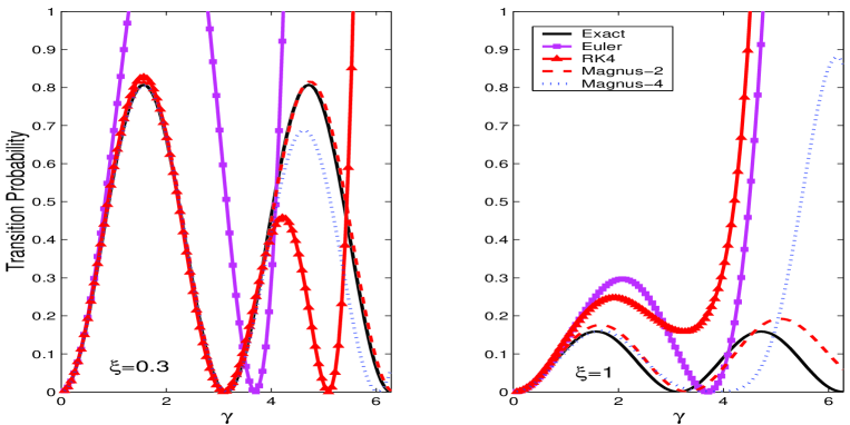
Figure 14: Rosen–Zener model: Transition probabilities as a function of $\gamma$, with $\xi=0.3$ and $\xi=1$. The curves are coded as follows. Solid line represents the exact result; E1: solid lines with squares; RK4: solid lines with triangles; M2: dashed lines; M4: dashed-broken lines (indistinguishable from exact result in left panel).

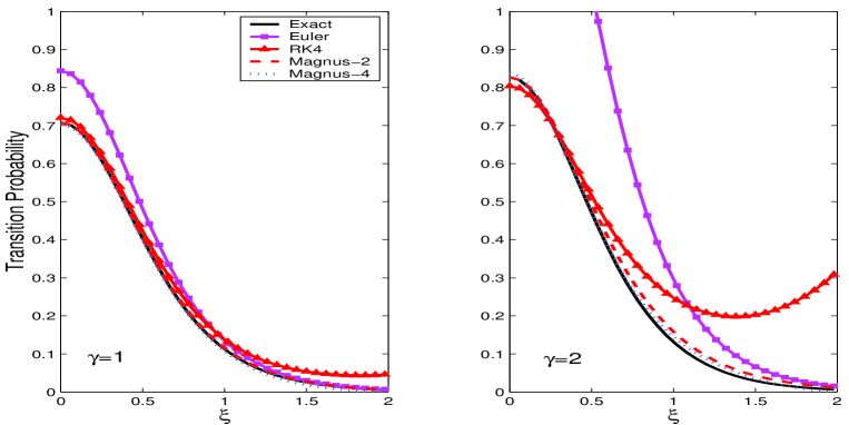
Figure 15: Rosen–Zener model: Transition probabilities as a function of $\xi$, with $\gamma=2$ and $\gamma=5$. Lines are coded as in Figure 14.

To increase the accuracy, one can always take smaller time steps, but then the number of evaluations of $A(t)$ increases, and this may be computationally very expensive for some problems due to the complexity of the time dependence and/or the size of the matrix. In those cases, it is important to have reliable numerical methods providing the desired accuracy as fast as possible or, alternatively, leading to the best possible accuracy at a given computational cost.

A good perspective of the overall performance of a given numerical integrator is provided by the so-called efficiency diagram. This efficiency plot is obtained by carrying out the numerical integration with different time steps, corresponding to different number of evaluations of $A(t)$. For each run one compares the corresponding approximation with the exact solution and plot the error as a function of the total number of matrix evaluations. The results are better illustrated in a double logarithmic scale. In that case, the slope of the curves should correspond, in the limit of very small time steps, to (minus) the order of accuracy of the method.

To illustrate this issue, in Figure 16 we collect the efficiency plots of the previous schemes when $\xi=0.3$ with $\gamma=10$ (left) and $\gamma=100$ (right). We have also included the results obtained by several higher order integrators, namely the sixth-order RK method (RK6) whose coefficients are collected in (229) and the sixth-order Magnus integrator (M6) given by (5.4) and (274). We clearly observe that the Euler method is, by far, the worst choice if accurate results are desired. Notice the (double) logarithmic scale of the plots: thus, for instance, when $\gamma=10$ the range goes approximately from 300 to 3000 evaluations of $A(t)$. Magnus integrators, in addition to providing results in $\mathrm{SU}(2)$ by construction (as the exact solution), show a better efficiency than Runge–Kutta schemes for these examples, and this efficiency increases with the value of $\gamma$ considered. The implicit Runge-Kutta-Gauss-Legendre methods (254) show slightly better results than the explicit RK methods, but still considerably worst than Magnus integrators.

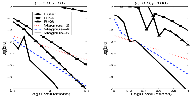
Figure 16: Rosen–Zener model: Error in the transition probabilities versus the number of evaluations of the Hamiltonian $H_{I}(s)$ for $\xi=0.3$ and $\gamma=10$ (left panel) and $\gamma=100$ (right panel).

If we compare Magnus integrators of different orders of accuracy, we observe that the most efficient scheme is the second order method M2 when relatively low accuracies are desired. For higher accuracy, however, it is necessary to carry out a thorough analysis of the computational cost of the methods for a given problem before asserting the convenience of M4 or M6 with respect to higher order schemes. For a fixed time step $h$, the computational cost of a certain family of methods (such as those based on Magnus) usually increases with the order. However, if one fixes the number of $A(t)$ evaluations, this is not necessarily the case (sometimes higher order methods requires more commutators but less exponentials).

Let us now compare the performance of the Magnus methods with respect to other Lie-group solvers, namely Fer and Cayley methods. We repeat the same experiments as in Fig. 16 but, for clarity, only the results for the 6th-order methods are shown. We consider the symmetric-Fer method given by (282) and (5.4.2) and the Cayley method (286) with (289) using in both cases the Gauss–Legendre quadrature. The results obtained are collected in Figure 17. We clearly observe that the relative performance of the Cayley method deteriorates by increasing the value of $\gamma$ similarly to the RK6. In spite of preserving the qualitative properties, this example shows that for some problems, polynomial or rational approximations do not perform efficiently. Here, in particular, the Magnus scheme is slightly more efficient that the symmetric Fer method, although for other problems their performance is quite similar.

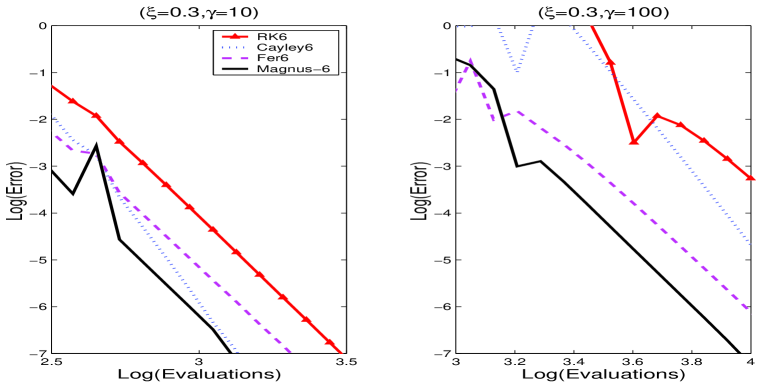
Figure 17: Rosen–Zener model: Same as Figure 16 where we compare the performance of the 6th-order Magnus, symmetric-Fer, Cayley and RK6.

5.6 Computing the exponential of a matrix

We have seen that the numerical schemes based on the Magnus expansion provide excellent results when applied to equation (223) with coefficient matrix (290). In fact, they are even more efficient than several Runge–Kutta algorithms. Of course, for this particular example the number of $A(t)$ evaluations is a good indication of the computational cost required by the numerical schemes, since the evaluation of $\exp(\Omega)$ can be done analytically by means of formula (18). In general, however, the matrix exponential has to be also approximated numerically and thus the performance of the numerical integration algorithms based on the Magnus expansion strongly depends on this fact. It may happen that the evaluation of $\exp(C)$, where $C$ is a (real or complex) $N\times N$ matrix, represents the major factor in the overall computational cost required by this class of algorithms and is probably one of their most problematic aspects.

As a matter of fact, the approximation of the matrix exponential is among the oldest and most extensively researched topics in numerical mathematics. Although many efficient algorithms have been developed, the problem is still far from been solved in general. It seems then reasonable to briefly summarize here some of the most widely used procedures in this context.

Let us begin with two obvious but important remarks. (i) First, one has to distinguish whether it is required to evaluate the full matrix $\exp(C)$ or only the product $\exp(C)v$ for some given vector $v$. In the later case, special algorithms can be designed requiring a much reduced computational effort. This is specially true when $C$ is large and sparse (as often happens with matrices arising from the spatial discretization of partial differential equations). (ii) Second, for the numerical integration methods based on ME one has to compute $\exp(C(h))$, where $C(h)=\mathcal{O}(h^{p})$, $h$ is a (not too large) step size and $p\geq 1$. In other words, the matrices to be exponentiated have typically a small norm (usually restricted by the convergence bounds of the expansion).

In any case, prior to the computation of $\exp(C)$, it is significant to have as much information about the exponent $C$ as possible. Thus, for instance, if the matrix $C$ resides in a Lie algebra, then $\exp(C)$ belongs to the corresponding Lie group and one has to decide whether this qualitative property has to be exactly preserved or constructing a sufficiently accurate approximation (e.g., at a higher order than the order of the integrator itself) is enough. Also when $C$ can be split into different parts, one may consider a factorization of the form $\exp(C)\approx\exp(C_{1})\exp(C_{2})\cdots\exp(C_{m})$ if each individual exponential is easy to evaluate exactly.

An important reference in this context is [177] and its updated version [178], where up to nineteen (or twenty in [178]) different numerical algorithms for computing the exponential of a matrix are carefully reviewed. An extensive software package for computing the matrix exponential is Expokit, developed by R. Sidje, with Fortran and Matlab versions available [214, 215]. In addition to computing the matrix-valued function $\exp(C)$ for small, dense matrices $C$, Expokit has functions for computing the vector-valued function $\exp(C)v$ for both small, dense matrices and large, sparse matrices.

5.6.1 Scaling and squaring with Padé approximation

Among one of the least dubious ways of computing $\exp(C)$ is by scaling and squaring in combination with a diagonal Padé approximation [178]. The procedure is based on a fundamental property of the exponential function, namely

$$\e^{C}=(\e^{C/j})^{j}$$

for any integer $j$. The idea then is to choose $j$ to be a power of two for which $\exp(C/j)$ can be reliably and efficiently computed, and then to form the matrix $(\exp(C/j))^{j}$ by repeated squaring. If the integer $j$ is chosen as the smallest power of two for which $\|C\|/j<1$, then $\exp(C/j)$ can be satisfactorily computed by diagonal Padé approximants of order, say, $m$. This is roughly the method used by the built-in function expm in Matlab.

For the integrators based on the Magnus expansion, as $C=\mathcal{O}(h^{p})$ with $p\geq 1$, one usually gets good approximations with relatively small values of $j$ and $m$.

As is well known, diagonal Padé approximants map the Lie algebra $\mathrm{o}_{J}(n)$ to the $J$-orthogonal Lie group $\mathrm{O}_{J}(n)$ and thus constitute also a valid alternative to the evaluation of the exponential matrix in Magnus-based methods for this particular Lie group. More specifically, if $B\in\mathrm{o}_{J}(n)$, then $\psi_{2m}(tB)\in\mathrm{O}_{J}(n)$ for sufficiently small $t\in\mathbb{R}$, with

$$\psi_{2m}(\lambda)=\frac{P_{m}(\lambda)}{P_{m}(-\lambda)},$$ (294)

provided the polynomials $P_{m}$ are generated according to the recurrence

$$P_{0}(\lambda) = 1,\ \qquad P_{1}(\lambda)=2+\lambda$$

$$P_{m}(\lambda) = 2(2m-1)P_{m-1}(\lambda)+\lambda^{2}P_{m-2}(\lambda).$$

Moreover, $\psi_{2m}(\lambda)=\exp(\lambda)+\mathcal{O}(\lambda^{2m+1})$ and $\psi_{2}$ corresponds to the Cayley transform (279), whereas for $m=2,3$ we have

$$\psi_{4}(\lambda) = \left(1+\frac{1}{2}\lambda+\frac{1}{12}\lambda^{2}\right)\Big{/}\left(1-\frac{1}{2}\lambda+\frac{1}{12}\lambda^{2}\right)$$

$$\psi_{6}(\lambda) = \left(1+\frac{1}{2}\lambda+\frac{1}{10}\lambda^{2}+\frac{1}{120}\lambda^{3}\right)\Big{/}\left(1-\frac{1}{2}\lambda+\frac{1}{10}\lambda^{2}-\frac{1}{120}\lambda^{3}\right).$$

Thus, we can combine the optimized approximations to $\Omega$ obtained in subsection 5.4 for Magnus based methods with diagonal Padé approximants up to the corresponding order to obtain time-symmetric integration schemes preserving the algebraic structure of the problem without computing the matrix exponential. For instance, the “Magnus–Padé” methods thus obtained involve, in addition to one matrix inversion, 3 and 8 matrix-matrix products for order 4 and 6, respectively.

Observe that since $\Omega^{[2n]}=\mathcal{O}(h)$ then

$$\psi_{2m}(\Omega^{[2n]})=\exp(\Omega^{[2n]})+\mathcal{O}(h^{2k+1}),$$

where $k=\min\{m,n\}$. With $m=n$ we have a method of order $2n$. However, for some problems this rational approximation to the exponential may be not very accurate depending on the eigenvalues of $\Omega^{[2n]}$. In this case one may take $m>n$, thus giving a better approximation to the exponential and a more accurate result by increasing slightly the computational cost of the method. Of course, when the norm of the matrix $\Omega^{[2n]}$ is not so small, this technique can be combined with scaling and squaring [70].

Instead of using Padé approximants for the exponential of the scaled matrix $B\equiv C/2^{k}$, Najfeld and Havel [188] propose a rational approximation for the matrix function

$$H(B)=B\coth(B)=B\,\frac{\e^{2B}+I}{\e^{2B}-I},$$ (295)

from which the exponential can be obtained as

$$\e^{2B}=\frac{H(B)+B}{H(B)-B}$$

and then iteratively square the result $k$ times to recover the exponential of the original matrix $C$. From the continued fraction expansion of $H(B)$, it is possible to compute the first rational approximations as

$$H_{2}(B)=\frac{I+\frac{2}{5}B^{2}}{I+\frac{1}{15}B^{2}},\qquad H_{4}(B)=\frac{I+\frac{4}{9}B^{2}+\frac{1}{63}B^{4}}{I+\frac{1}{9}B^{2}+\frac{1}{945}B^{4}}$$

and so on. Observe that the representation (295) can be regarded as a generalized Cayley transform of $B$ and thus it also provides approximations in the group $\mathrm{O}_{J}(n)$. In [188] the authors report a saving of about 30% in the number of matrix multiplications with respect to diagonal Padé approximants when an optimal $k$ and a rational approximation for $H(B)$ is used.

5.6.2 Chebyshev approximation

Another valid alternative is to use polynomial approximations to the exponential of $C$ as a whole. Suppose, in particular, that $C$ is a matrix of the form $C=-i\tau H$, with $H$ Hermitian and $\tau>0$, as is the case in Quantum Mechanics. In the Chebyshev approach, the evolution operator $\exp(-i\tau H)$ is expanded in a truncated series of Chebyshev polynomials, in analogy with the approximation of a scalar function [223]. As is well known, given a function $F(x)$ in the interval $[-1,1]$, the Chebyshev polynomial approximations are optimal, in the sense that the maximum error in the approximation is minimal compared to almost all possible polynomial approximations [221]. To apply this procedure, one has to previously bound the extreme eigenvalues $E_{\mathrm{min}}$ and $E_{\mathrm{max}}$ of $H$. Then a truncated Chebyshev expansion of $\exp(-ix)$ on the interval $[\tau E_{\mathrm{min}},\tau E_{\mathrm{max}}]$ is considered:

$$\exp(-ix)\approx\sum_{n=0}^{m}c_{n}P_{n}(x),$$

where

$$P_{n}(x)=T_{n}\left(\frac{2x-\tau E_{\mathrm{max}}-\tau E_{\mathrm{min}}}{\tau E_{\mathrm{max}}-\tau E_{\mathrm{min}}}\right)$$

with appropriately chosen coefficients $c_{n}$. Here $T_{n}(x)$ are the Chebyshev polynomials on the interval $[-1,1]$ [2], which can be determined via the recurrence relation

$$T_{n+1}(x)=2xT_{n}(x)-T_{n-1}(x);\quad T_{1}(x)=x;\quad T_{0}(x)=1.$$

Finally, one uses the approximation

$$\exp(-i\tau H)\approx\sum_{n=0}^{m}c_{n}P_{n}(\tau H).$$ (296)

This technique is frequently used in numerical quantum dynamics to compute $\exp(-i\tau H)\psi_{0}$ over very long times. This can be done with $m$ matrix-vector products if the approximation (296) is considered with a sufficiently large truncation index $m$. In fact, the degree $m$ necessary for achieving a specific accuracy depends linearly on the step size $\tau$ and the spectral radius of $H$ [189], and thus an increase of the step size reduces the computational work per unit step. In a practical implementation, $m$ can be chosen such that the accuracy is dominated by the round-off error [145]. This approach has two main drawbacks: (i) it is not unitary, and therefore the norm is not conserved (although the deviation from unitarity is really small due to its extreme accuracy), and (ii) intermediate results are not obtained, since typically $\tau$ is very large.

5.6.3 Krylov space methods

As we have already pointed out, very often what is really required, rather than the exponential of the matrix $C$ itself, is the computation of $\exp(C)$ applied to a vector. In this situation, evaluating $\e^{C}$ is somehow analogous to computing $C^{-1}$ to get the solution of the linear system of equations $Cx=b$ for many different $b$’s: other procedures are clearly far more desirable. The computation of $\e^{C}v$ can be efficiently done with Krylov subspace methods, in which approximations to the solution are obtained from the Krylov spaces spanned by the vectors $\{v,Cv,C^{2}v,\ldots,C^{j}v\}$ for some $j$ that is typically small compared to the dimension of $C$ [71, 194]. The Lanczos method for solving iteratively symmetric eigenvalue problems is of this form [233]. If, as before, we let $C=-i\tau H$, the symmetric Lanczos process generates recursively an orthonormal basis $V_{m}=[v_{1}\cdots v_{m}]$ of the $m$th Krylov subspace $K_{m}(H,u)=\mathrm{span}(u,Hu,\ldots,H^{m-1}u)$ such that

$$HV_{m}=V_{m}L_{m}+[0\cdots 0\,\beta_{m}\,v_{m+1}],$$

where the symmetric tridiagonal $m\times m$ matrix $L_{m}=V^{T}_{m}HV_{m}$ is the orthogonal projection of $H$ onto $K_{m}(H,u)$. Finally,

$$\exp(-i\tau H)u\approx V_{m}\exp(-i\tau L_{m})V_{m}^{T}u$$

and the matrix exponential $\exp(-i\tau L_{m})$ can be computed by diagonalizing $L_{m}$, $L_{m}=Q_{m}D_{m}Q_{m}^{T}$, as

$$\exp(-i\tau L_{m})=Q_{m}\exp(-i\tau D_{m})Q_{m}^{T},$$

with $D_{m}$ a diagonal matrix. This iterative process is stopped when

$$\beta_{m}\left\|\left(\exp(-i\tau L_{m})\right)_{m,m}\right\|<tol$$

for a fixed tolerance. Very good approximations are often obtained with relatively small values of $m$, and computable error bounds exist for the approximation. This class of schemes require generally $\mathcal{O}(N^{2})$ floating point operations in the computation of $\e^{C}v$. More details are contained in the references [103, 105, 106].

5.6.4 Splitting methods

Frequently, one has to exponentiate a matrix which can be split into several parts which are either solvable or easy to deal with. Let us assume for simplicity that $C=A+B$, where the computation $\e^{C}$ is very expensive, but $\e^{A}$ and $\e^{B}$ are cheap and easy to evaluate. In such circumstances, it makes sense to approximate $\e^{\varepsilon C}$ with $\varepsilon$ a small parameter, by the following scheme:

$$\psi^{[p]}_{h}\equiv\e^{\varepsilon b_{m}B}\e^{\varepsilon a_{m}A}\ \cdots\ \e^{\varepsilon b_{1}B}\e^{\varepsilon a_{1}A}\ =\e^{\varepsilon(A+B)}+\mathcal{O}(\varepsilon^{p+1})$$ (297)

with appropriate parameters $a_{i},b_{i}$. This can be seen as the approximations to the solution at $t=\varepsilon$ of the equation $Y^{\prime}=(A+B)Y$ by a composition of the exact solutions of the equations $Y^{\prime}=AY$ and $Y^{\prime}=BY$ at times $t=a_{i}\varepsilon$ and $t=b_{i}\varepsilon$, respectively. Two instances of this kind of approximations are given by the well known Lie–Trotter formula

$$\psi^{[1]}_{h}=\e^{\varepsilon A}\e^{\varepsilon B}$$ (298)

and the second order symmetric composition

$$\psi^{[2]}_{h}=\e^{\varepsilon A/2}\e^{\varepsilon B}\e^{\varepsilon A/2},$$ (299)

referred to as Strang splitting, Störmer, Verlet and leap-frog, depending on the particular area where it is used.

Splitting methods have been considered in different contexts: in designing symplectic integrators, for constructing volume-preserving algorithms, in the numerical integration of partial differential equations, etc. An extensive survey of the theory and practice of splitting methods can be found in [27, 99, 146, 165, 166] and references therein.

Splitting methods are particularly useful in geometric numerical integration. Suppose that the matrix $C=A+B$ resides in a Lie algebra $\mathfrak{g}$. Then, obviously, $\exp(C)$ belongs to the corresponding Lie group $\mathcal{G}$ and one is naturally interested in getting approximations also in $\mathcal{G}$. In this respect, notice that if $A,B\in\mathfrak{g}$, then the scheme (297) also provides an approximation in $\mathcal{G}$. It is worth noticing that other methods for the approximation of the matrix exponential, e.g., Padé approximants and Krylov subspace techniques, are not guaranteed to map elements from $\mathfrak{g}$ to $\mathcal{G}$. Although diagonal Padé approximants map the Lie algebra $\mathrm{o}_{J}$ to the underlying group, it is possible to show that the only analytic function that maps $\mathfrak{sl}(n)$ into the special linear group $\mathrm{SL}(n)$ approximating the exponential function up to a given order is the exponential itself [84]. In consequence, diagonal Padé approximants only provide results in $\mathrm{SL}(n)$ if the computation is accurate to machine precision.

In [46], Celledoni and Iserles devised a splitting technique for obtaining an approximation to $\exp(C)$ in the Lie group $\mathcal{G}$ based on a decomposition of $C\in\mathfrak{g}$ into low-rank matrices $C_{i}\in\mathfrak{g}$. Basically, given a $n\times n$ matrix $C\in\mathfrak{g}$, they proposed to split it in the form

$$C=\sum_{i=1}^{k}C_{i},$$

such that

1. $C_{i}\in\mathfrak{g}$, for $i=1,\ldots,k$.

2. Each $\exp(C_{i})$ is easy to evaluate exactly.

3. Products of such exponentials are computationally cheap.

For instance, for the Lie algebra $\mathfrak{so}(n)$, the choice

$$C_{i}=\frac{1}{2}c_{i}e_{i}^{T}-\frac{1}{2}e_{i}b_{i}^{T},\qquad i=1,\ldots,n,$$

where $c_{1},\ldots,c_{n}$ are the columns of $C$ and $e_{i}$ is the $i$-th vector of the canonical basis of $\mathbb{R}^{n}$, satisfies the above requirements (with $k=n$), whereas in the case of $\mathfrak{g}=\mathfrak{sl}(n)$ other (more involved) alternatives are possible [46].

Proceeding as in (298), with

$$\psi^{[1]}=\exp(\varepsilon C_{1})\exp(\varepsilon C_{2})\cdots\exp(\varepsilon C_{k})$$

we get an order one approximation in $\varepsilon$ to $\exp(\varepsilon C)$, whereas the symmetric composition

$$\psi^{[2]}=\e^{\frac{1}{2}\varepsilon C_{k}}\e^{\frac{1}{2}\varepsilon C_{k-1}}\cdots\e^{\frac{1}{2}\varepsilon C_{2}}\e^{\varepsilon C_{1}}\e^{\frac{1}{2}\varepsilon C_{2}}\cdots\e^{\frac{1}{2}\varepsilon C_{k-1}}\e^{\frac{1}{2}\varepsilon C_{k}}$$ (300)

provides an approximation of order two in $\varepsilon$, and this can be subsequently combined with different techniques for increasing the order.

With respect to the computational cost, the results reported in [46] show that, up to order four in $\varepsilon$, this class of splitting schemes are competitive with the Matlab built-in function expm when machine accuracy is not required in the final approximation. Running expm on randomly generated matrices, it is possible to verify that computing $\exp(C)$ to machine accuracy requires about (20-30)$n^{3}$ floating point operations, depending on the eigenvalues of $C$, whereas the 4th-order method constructed from (300) involves (12-15)$n^{3}$ operations when $C\in\mathfrak{so}(100)$ [46]. In the case of the approximation of $\exp(C)v$ and $v\in\mathbb{R}^{n}$, the cost of low-rank splitting methods drop down to $Kn^{2}$, where $K$ is a constant, and thus they are comparable to those achieved by polynomial approximants [106].

Splitting methods of the above type are by no means the only way to express $\exp(C)$ as a product of exponentials of elements in $\mathfrak{g}$. For instance, the Wei–Norman approach (111) can also be implemented in this setting. Suppose that $\dim\mathfrak{g}=s$ and let $\{X_{1},X_{2},\ldots,X_{s}\}$ be a basis of $\mathfrak{g}$. In that case, as we have seen (subsection 2.10.3), it is possible to represent $\exp(tC)$ for $C\in\mathfrak{g}$ and sufficiently small $|t|$ in canonical coordinates of the second kind,

$$\e^{tC}=\e^{g_{1}(t)X_{1}}\,\e^{g_{2}(t)X_{2}}\cdots\e^{g_{s}(t)X_{s}},$$

where the scalar functions $g_{k}$ are analytic at $t=0$. Although the $g_{k}$s are implicitly defined, they can be approximated by Taylor series. The cost of the procedure can be greatly reduced by choosing adequately the basis and exploiting the Lie-algebraic structure [47].

Yet another procedure to get approximations of $\exp(C)$ in a Lie-algebraic setting which has received considerable attention during the last years is based on generalized polar decompositions (GPD), an approach introduced in [183] and further elaborated in [123, 245]. In particular, in [123], by bringing together GPD with techniques from numerical linear algebra, new algorithms are presented with complexity $\mathcal{O}(n^{3})$, both when the exponential is applied to a vector and to a matrix. This is certainly not competitive with Krylov subspace methods in the first case, but represents at least a 50% improvement on the execution time, depending on the Lie algebra considered, in the latter. Another difference with respect to Krylov methods is that the algorithms based on generalized polar decompositions approximate the exponential to a given order of accuracy and thus they are well suited to exponential approximations within numerical integrators for ODEs, since the error is subsumed in that of the integration method. For a complete description of the procedure and its practical implementation we refer the reader to [123].

5.7 Additional numerical examples

The purpose of subsection 5.5 was to illustrate the main features of the numerical schemes based on the Magnus expansion in comparison with other standard integrators (such as Runge–Kutta schemes) and other Lie-group methods (e.g., Fer and Cayley) on a solvable system. For larger systems the efficiency analysis is more challenging since the (exact or approximate) computation of exponential matrices play an important role on the performance of the methods. It makes sense then to analyze from this point of view more realistic problems where one necessarily has to approximate the exponential in a consistent way.

As an illustration of this situation we consider next two skew-symmetric matrices $A(t)$ and $Y(0)=I$, so that the solution $Y(t)$ of $Y^{\prime}=A(t)Y$ is orthogonal for all $t$. In particular, the upper triangular elements of the matrices $A(t)$ are as follows:

$$\mbox{(a)}\;\;\;A_{ij} = \sin\left(t(j^{2}-i^{2})\right)\qquad\qquad 1\leq i<j\leq N$$ (301)

$$\mbox{(b)}\;\;\;A_{ij} = \log\left(1+t\,\frac{j-i}{j+i}\right)$$ (302)

with $N=10$. In both cases $Y(t)$ oscillates with time, mainly due to the time-dependence of $A(t)$ (in (301)) or the norm of the eigenvalues (in (302)).

The integration is carried out in the interval $t\in[0,10]$ and the approximate solutions are compared with the exact one at the final time $t_{\mathrm{f}}=10$ (obtained with very high accuracy by using a sufficiently small time step). The corresponding error at $t_{\mathrm{f}}$ is computed for different values of the time step $h$. The Lie-group solvers are implemented with Gauss–Legendre quadratures and constant step size.

First, we plot the accuracy of the different 4-th and 6-th order methods as a function of the number of $A(t)$ evaluations. In contrast to the previous examples, now there is not a closed formula for the matrix exponentials appearing in the Magnus based integrators, so that some alternative procedure must be applied. In particular, the computation of $\e^{C}$ to machine accuracy is done by scaling–(diagonal Padé)–squaring, so that the result is correct up to round-off. Figure 18 shows the results obtained for the problems (301) and (302) with fourth- and sixth-order numerical schemes based on Magnus and Cayley, and also explicit Runge–Kutta methods. In the first problem, Magnus and Cayley show a very similar performance, which happens to be only slightly better than that of RK methods.

The situation changes drastically, however, for the second problem. Here the behaviour of Cayley and RK methods is essentially similar, whereas schemes based on Magnus are clearly more efficient. The reason seems to be that Cayley and RK methods give poor approximations to the exponential, which, on the other hand, has to be accurately approximated, since the eigenvalues of $A(t)$ may take large values.

With respect to symmetric Fer methods, their efficiency is quite similar to that of Magnus if the matrix exponentials are evaluated accurately up to machine precision. This is so for the matrix (301) even if Padé approximants of relatively low order are used to replace the exponentials.

On the other hand, the efficiency of “Magnus-Padé” methods (we denote by MP$nm$ a Magnus method of order $n$ where the exponential is approximated by a diagonal Padé of order $m$, and MP$n$ if $n=m$) is highly deteriorated for the problem (302), although it is always better than the corresponding to Cayley schemes.

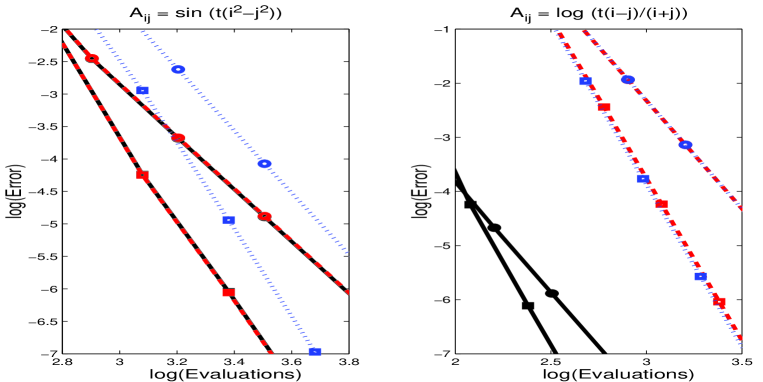
Figure 18: Efficiency diagram corresponding to the optimized 4-th (circles) and 6-th (squares) order Lie-group solvers based on Magnus (solid lines) and Cayley (broken lines), and the standard Runge–Kutta methods (dashed lines).

To better illustrate all these comments, in Figure 19 we display the error in the solution corresponding to (301) and (302) as a function of time in the interval $t\in[0,100]$ for $h=1/20$ as is obtained by the previous methods. We should stress that all schemes require the same number of $A$ evaluations.

In the right picture the exponentials appearing in the Magnus method are computed using a Padé approximant of order six (MP6), of order eight (MP68) and to machine accuracy (M6). Observe the great importance of evaluating the exponential as accurately as possible for the matrix (302): by increasing slightly the computational cost per step in the computation of the matrix exponential it is possible to improve dramatically the accuracy of the methods. On the contrary, for problem (301) the meaningful fact seems to be that the integration scheme provides a solution in the corresponding Lie group.

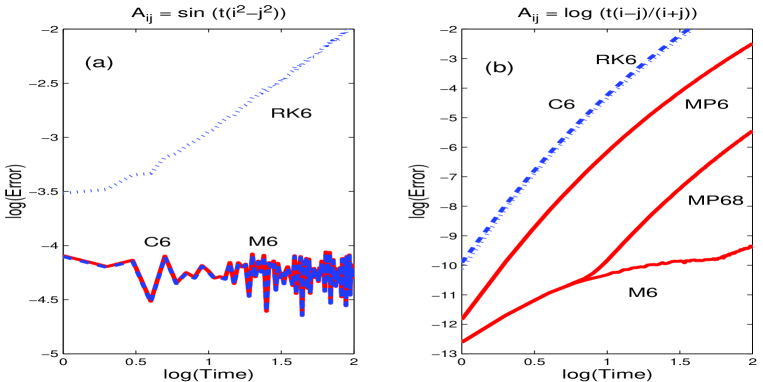
Figure 19: Error as a function of time (in logarithmic scale) obtained with different 6-th order integrators for $h=1/20$: (a) problem (301); (b) problem (302).

5.8 Modified Magnus integrators

5.8.1 Variations on the basic algorithm

The examples collected in subsections 5.5 and 5.7 show that the numerical methods constructed from the Magnus expansion can be computationally very efficient indeed. It is fair to say, however, that this efficiency can be seriously affected when dealing with certain types of problems.

Suppose, for instance, that one has to numerically integrate a problem defined in $\mathrm{SU}(n)$. Although Magnus integrators are unconditionally stable in this setting (since they preserve unitarity up to roundoff independently of the step size $h$), in practice only small values of $h$ are used for achieving accurate results. Otherwise the convergence of the series is not assured. Of course, the use of small time steps may render the algorithm exceedingly costly.

In other applications the problem depends on several parameters, so that the integration has to be carried out for different values of the parameters. In that case the overall integration procedure can be computationally very expensive.

In view of all these difficulties, it is hardly surprising that several modifications of the standard algorithm of Magnus integrators had been developed to try to minimize these undesirable effects and get especially adapted integrators for particular problems.

One basic tool used time and again in this context is performing a preliminary linear transformation, similarly to those introduced in section 2.9. These transformations can be carried out either for the whole integration interval or at each step in the process. Given an appropriately chosen transformation, $\tilde{Y}_{0}(t)$, one factorizes $Y(t)=\tilde{Y}_{0}(t)\,\tilde{Y}_{1}(t)$, where the unknown $\tilde{Y}_{1}(t)$ satisfies the equation

$$\tilde{Y}_{1}^{\prime}=B(t)\tilde{Y}_{1}$$ (303)

and $B(t)$ depends on $A(t)$ and $\tilde{Y}_{0}(t)$. This transformation makes sense, of course, if $\|B(t)\|<\|A(t)\|$ and thus typically $\tilde{Y}_{0}$ is chosen in such a way that the norm of $B$ verifies the above inequality. As a consequence, Magnus integrators can be applied on (303) with larger time steps providing also more accurate results.

Alternatively, for problems where in addition to the time step $h$ there is another parameter ($E$, say), one may analyze the Magnus expansion in terms of $h$ and $E$. This allows us to identify which terms at each order in the series expansion give the main contribution to the error, and design methods which include these terms in their formulation. The resulting schemes should provide then more accurate results at a moderate computational cost without altering the convergence domain. As a general rule, it is always desirable to have in advance as much information about the equation and the properties of its solution as possible, and then to try to incorporate all this information into the algorithm.

Let us review some useful possibilities in this context. From (258) one has

$$A(t)=a_{0}+\tau a_{1}+\tau^{2}a_{2}+\cdots,$$ (304)

where $\tau=t-t_{1/2}$. The first term is exactly solvable ($a_{0}=A(t_{1/2})$) and, for many problems, it just provides the main contribution to the evolution of the system. In that case it makes sense to take

$$\tilde{Y}_{0}(t)=\e^{(t-t_{n})a_{0}}=\e^{(t-t_{n})A(t_{1/2})}$$

and subsequently integrate eq. (303) with

$$B(t)=\e^{-(t-t_{n})A(t_{1/2})}\left(A(t)-A(t_{1/2})\right)\e^{(t-t_{n})A(t_{1/2})}.$$

This approach has been considered in [115, 116], and shows an extraordinary improvement when the system is highly oscillatory and the main oscillatory part is integrated with $\tilde{Y}_{0}$. In those cases, the norm of $B(t)$ is considerably smaller than $\|A(t)\|$, but $B(t)$ is still highly oscillatory, so that especially adapted quadrature rules have to be used in conjunction with the Magnus expansion [117, 121].

In some other problems the contributions from the derivatives can also be significant, so that a more appropriate transformation is defined by

$$\tilde{Y}_{0}(t)=\exp\left(\int_{t_{n}}^{t}A(\tau)d\tau\right).$$ (305)

The resulting methods can be considered then as a combination of the Fer or Wilcox expansions and the Magnus expansion. This approach has been pursued in [61].

On the other hand, it is known that several physically relevant systems evolve adiabatically or almost-adiabatically. In that case it seems appropriate to consider the adiabatic picture which instantaneously diagonalizes $A(t)$ (subsection 2.9). This analysis is carried out in [124, 125, 151]. In [125] the adiabatic picture is used perturbatively, whereas in [124] it is shown that Magnus in the new picture leads to significant improvements.

Alternatively, one can analyze the structure of the leading error terms in order to identify the main contribution to the error at each $\Omega_{i}$ in the Magnus series expansion. In most cases they correspond to terms involving only $\alpha_{1}$ and its nested commutators with $\alpha_{2}$ Thus, in particular, the standard fourth-order method given by (260) can be easily improved by including the dominant error term at higher orders, i.e.,

$$\Omega^{[4]}=\alpha_{1}-\frac{1}{12}[\alpha_{1},\alpha_{2}]+\frac{1}{720}[\alpha_{1},\alpha_{1},\alpha_{1},\alpha_{2}]-\frac{1}{30240}[\alpha_{1},\alpha_{1},\alpha_{1},\alpha_{1},\alpha_{1},\alpha_{2}]+\ldots.$$

We recall that using the fourth-order Gauss–Legendre quadrature rule we can take $\alpha_{1}=\frac{h}{2}(A_{1}+A_{2}),\ \alpha_{2}=\frac{h\sqrt{3}}{12}(A_{2}-A_{1})$ with $A_{1},A_{2}$ given in (269). The new method requires additional commutators but the accuracy can be improved a good deal. This procedure is analyzed in [172], where it is shown how to sum up all terms of the form $[\alpha_{1},\alpha_{1},\ldots,\alpha_{1},\alpha_{2}]$. An error analysis in the limit of very large values of $\|\alpha_{1}\|$ is done in [5, 160].

5.8.2 Commutator-free Magnus integrators

All numerical methods based on the Magnus expansion appearing in the preceding sections require the evaluation of a matrix exponential which contain several nested commutators. As we have repeatedly pointed out, computing the exponential is frequently the most consuming part of the algorithm. There are problems where the matrix $A(t)$ has a sufficiently simple structure which allows one to approximate efficiently the exponential $\exp(A(t_{i}))$, or the exponential of a linear combination of the matrix $A(t)$ evaluated at different points. In some sense, this is equivalent to have efficient methods to compute or to approximate $\tilde{Y}_{0}$ in (305). It may happen, however, that the computation of the matrix exponential is a much more involved task due to the presence of commutators in the Magnus expansion. For this reason, it makes sense to look for approximations to the Magnus expansion which do not involve commutators whilst still preserving the same qualitative properties. In other words, one may be interested in compositions of the form

$$\Psi^{[n]}_{m}\equiv\exp\left(\int_{t_{n}}^{t_{n}+h}p_{m}(s)A(s)ds\right)\ \cdots\ \exp\left(\int_{t_{n}}^{t_{n}+h}p_{1}(s)A(s)ds\right)$$ (306)

where $p_{i}(s)$ are scalar functions chosen in such a way that $\Psi^{[n]}_{m}=\e^{\Omega(t_{n}+h)}+\mathcal{O}(h^{n+1})$. Alternatively, instead of the functions $p_{i}(s)$, it is possible to find coefficients $\varrho_{i,j},\ i=1,\ldots,m,j=1,\ldots,k$ such that

$$\Psi^{[n]}_{m}\equiv\e^{\tilde{A}_{m}}\cdots\e^{\tilde{A}_{1}},\qquad\mbox{with}\qquad\tilde{A}_{i}=h\sum_{j=1}^{k}\varrho_{i,j}A_{j}$$ (307)

is an approximation of the same order. This procedure requires first to compute $A_{j}=A(t_{n}+c_{j}h),\ j=1,\ldots,k$ for some quadrature nodes, $c_{j}$, of order $n$ or higher and, obviously, the coefficients $\varrho_{i,j}$ will depend on this choice. The process simplifies if one works in the associated graded free Lie algebra generated by $\{\alpha_{i}\}$, as in the sequel of eq. (5.4). Thus, achieving fourth-order integrators reduces just to solve the equations for the new coefficients $a_{i,1},a_{i,2}$ in

$$\Psi^{[4]}_{m} \equiv \exp\left(a_{m,1}\,\alpha_{1}+a_{m,2}\,\alpha_{2}\right)\cdots\exp\left(a_{1,1}\,\alpha_{1}+a_{1,1}\,\alpha_{2}\right)$$ (308)

with the requirement that $\Psi^{[4]}_{m}=\exp\left(\Omega^{[4]}\right)+O(h^{5})$, where $\Omega^{[4]}$ is given by (260). Here the dependence of $a_{i,1},a_{i,2}$ on the coefficients $\varrho_{i,j}$ is determined through the existing relation between the $\alpha_{i}$ and the $A_{j}$ given in (267). The order conditions for the coefficients $a_{i,1},a_{i,2}$ can be easily obtained from the Baker–Campbell–Hausdorff formula. As we have already mentioned, time-symmetry is an important property to be preserved by the integrators, whereas, at the same time, also simplifies the analysis. Scheme (308) is time-symmetric if

$$a_{m+1-i,1}=a_{i,1},\qquad a_{m+1-i,2}=-a_{i,2},,\qquad i=1,2,\ldots,m$$ (309)

in which case the order conditions at even order terms are automatically satisfied. As an illustration, the simple compositions

$$\Psi^{[4]}_{2} \equiv \exp\left(\frac{1}{2}\alpha_{1}+\frac{1}{6}\alpha_{2}\right)\ \exp\left(\frac{1}{2}\alpha_{1}-\frac{1}{6}\alpha_{2}\right)$$ (310)

$$\Psi^{[4]}_{3} \equiv \exp\left(\frac{1}{12}\alpha_{2}\right)\ \exp\left(\alpha_{1}\right)\ \exp\left(-\frac{1}{12}\alpha_{2}\right)$$ (311)

are in fact fourth-order (commutator-free) methods requiring two and three exponentials, respectively [25]. In particular, scheme (310), when $\alpha_{1},\alpha_{2}$ are approximated using the fourth-order Gauss–Legendre quadrature as shown in (269) and (270) leads to the scheme

$$\Psi^{[4]}_{2}\equiv\exp\big{(}h(\varrho_{2,1}A_{1}+\varrho_{2,2}A_{2})\big{)}\ \exp\big{(}h(\varrho_{1,1}A_{1}+\varrho_{1,2}A_{2})\big{)}$$ (312)

with $\varrho_{1,1}=\varrho_{2,2}=\frac{1}{2}+\frac{\sqrt{3}}{72},\varrho_{1,2}=\varrho_{2,1}=\frac{1}{2}-\frac{\sqrt{3}}{72}$. Methods closely related to the scheme (311) are presented in [10, 25, 152], where they are applied to the Schrödinger equation with a time-dependent potential. A method quite similar to (310) is analyzed in [225] through its application to parabolic initial boundary value problems. A detailed study of fourth and sixth order commutator-free methods is presented in [28].

On the other hand, very often the differential equation (223) can be split into two parts, so that one has instead

$$Y^{\prime}=\big{(}A(t)+B(t)\big{)}Y,$$ (313)

where each part can be trivially or very efficiently solved. For instance, the Schrödinger equation with a time-dependent potential and, possibly, a time-dependent kinetic energy belongs to this class. In principle, the following families of geometric integrators are specially tailored for this problem:

I-

The commutator-free Magnus integrators (307), which in this case read

$$\Psi^{[n]}_{m}\equiv\e^{\tilde{A}_{m}+\tilde{B}_{m}}\cdots\e^{\tilde{A}_{1}+\tilde{B}_{1}},\qquad\mbox{with}\qquad\tilde{A}_{i}=h\sum_{j=1}^{k}\varrho_{i,j}A_{j},\ \ \tilde{B}_{i}=h\sum_{j=1}^{k}\varrho_{i,j}B_{j}.$$ (314)

Assuming that $\e^{\tilde{A}_{i}}$ and $\e^{\tilde{B}_{i}}$ are easily computed, then each exponential can be approximated by a conveniently chosen splitting method (297) [165]

$$\e^{\tilde{A}_{i}+\tilde{B}_{i}}\simeq\e^{b_{s}\tilde{B}_{i}}\e^{a_{s}\tilde{A}_{i}}\cdots\e^{b_{1}\tilde{B}_{i}}\e^{a_{1}\tilde{A}_{i}}.$$ (315)

II-

If one takes the time variable in $A(t),B(t)$ as two new coordinates, one may use any splitting method as follows [209]:

$$\Psi^{[n]}_{l,h}\equiv\e^{b_{l}hB(w_{l})}\e^{a_{l}hA(v_{l})}\cdots\e^{b_{1}hB(w_{1})}\e^{a_{1}hA(v_{1})},$$ (316)

with

$$v_{i}=\sum_{j=1}^{i-1}b_{j},\quad w_{i}=\sum_{j=1}^{i}a_{j}.$$

and $b_{0}=0,\ A(v_{i})\equiv A(t_{n}+v_{i}h),\ B(w_{i})\equiv B(t_{n}+w_{i}h)$.

Both approaches have pros and cons. By applying procedure I we may get methods of order $2n$ with only $n$ evaluations of $A(t)$, $B(t)$ using e.g. Gauss–Legendre quadratures, but if $m$ in (314) is large, the number of matrix exponentials to be computed leads to exceedingly costly methods. The approach II, on the other hand, has the advantage of a smaller number of stages, but also presents two drawbacks: (i) many evaluations of $A(t),B(t)$ are required in general; (ii) for matrices $A$ and $B$ with a particular structure there are specially designed splitting methods which are far more efficient, but these schemes are not easily adapted to this situation.

Next we show how to combine splitting methods with techniques leading to commutator free Magnus schemes to design efficient numerical algorithms possessing the advantages of approaches I and II, and at the same time generalizing the splitting idea (297) to this setting [19, 20].

The starting point is similar as in previous schemes, i.e. we consider a composition of the form

$$\psi_{l,h}^{[n]}=\e^{\tilde{B}_{l}}\ \e^{\tilde{A}_{l}}\cdots\e^{\tilde{B}_{1}}\ \e^{\tilde{A}_{1}},$$ (317)

where the matrices $\tilde{A}_{i}$ and $\tilde{B}_{i}$ are

$$\tilde{A}_{i}=h\sum_{j=1}^{k}\rho_{ij}A_{j},\qquad\tilde{B}_{i}=h\sum_{j=1}^{k}\sigma_{ij}B_{j},$$ (318)

with appropriately chosen real parameters $\rho_{ij},\sigma_{ij}$ depending on the coefficients of the chosen quadrature rule. Notice that $\e^{\tilde{A}_{i}}$ can be seen as the solution of the initial value problem $Y^{\prime}=\hat{A}_{i}Y$, $Y(t_{n})=I$ at $t_{n+1}$, where $\tilde{A}_{i}=h\hat{A}_{i}$. Of course, the same considerations apply to $\e^{\tilde{B}_{i}}$.

In many cases it is convenient to write the coefficients $\rho_{ij},\sigma_{ij}$ explicitly in terms of the coefficients $c_{i}$. Following [19] they can be written as

$$\rho_{ij}=\sum_{l=1}^{s}a_{i,l}\left(R^{(s)}Q_{X}^{(s,k)}\right)_{lj},\qquad\sigma_{ij}=\sum_{l=1}^{s}b_{i,l}\left(R^{(s)}Q_{X}^{(s,k)}\right)_{ij}.$$ (319)

where the coefficients for the matrices $R^{(s)},\ s=2,3$ are given in (266) and for $Q_{X}^{(s,k)}$ (whose elements depend on the coefficients $b_{i},c_{i}$ for the quadrature rule) as shown in (263).

In this way, the coefficients $a_{ij}$ and $b_{ij}$ are independent of the quadrature choice and can be obtained by solving some order conditions (see [19] for more details).

This procedure allows us to analyse separately particular cases for the matrices $A,B$ in order to build efficient methods. For instance, in [19] the following particular cases are considered: (i) when the matrices $A(t),B(t)$ have a general structure; (ii) when they satisfy the additional constraint $[B(t_{i}),[B(t_{j}),[B(t_{k}),A(t_{l})]]]=0$ as it happens, for instance, if $A$ corresponds to the kinetic energy and $B$ to the potential energy (both in classical or quantum mechanics).

As an illustration, we consider the following 4th-order 6-stage BAB composition

$$\psi_{6,h}^{[4]}=\e^{\tilde{B}_{7}}\ \e^{\tilde{A}_{6}}\ \e^{\tilde{B}_{6}}\cdots\e^{\tilde{A}_{1}}\ \e^{\tilde{B}_{1}}.$$ (320)

In Table 1 we collect the coefficients $a_{ij},b_{ij}$ to be used in (319) to obtain the coefficients $\rho_{ij},\sigma_{ij}$ to be used in the scheme (320) for two methods, denoted by $\mathrm{GS}_{6}$-4 in the general case (whose coefficients $a_{i1},b_{i1}$ correspond to $S_{6}$ in [27]) and $\mathrm{MN}_{6}$-4 when $[B(t_{i}),[B(t_{j}),[B(t_{k}),A(t_{l})]]]=0$ (the coefficients $a_{i1},b_{i1}$ correspond to $\mathrm{SRKN}_{6}^{b}$ in [27]).

Finally, one has to write the scheme in terms of the matrices $A_{i},B_{i}$. For instance, the composition (320) with the 4th-order Gauss–Legendre quadrature (i.e. taking $Q^{(2,2)}$ in (264) and $R^{(2)}$ in (266) to obtain the coefficients $\rho_{ij},\sigma_{ij}$ in (319)) gives

$$\tilde{A}_{i} = \left(\frac{1}{2}a_{i1}-\sqrt{3}a_{i2}\right)hA_{1}+\left(\frac{1}{2}a_{i1}+\sqrt{3}a_{i2}\right)hA_{2}$$

$$\tilde{B}_{i} = \left(\frac{1}{2}b_{i1}-\sqrt{3}b_{i2}\right)hB_{1}+\left(\frac{1}{2}b_{i1}+\sqrt{3}b_{i2}\right)hB_{2}.$$ (321)

Table 1: Splitting methods of order 4 for separable non-autonomous systems. $\mathrm{GS}_{6}$-4 is intended for general separable problems, whereas $\mathrm{MN}_{6}$-4 can be applied when $[B(t_{i}),[B(t_{j}),[B(t_{k}),A(t_{l})]]]=0$. All the coefficients are given in terms of $b_{11},a_{11},b_{21},a_{21},b_{31}$ for each method.

$\mathrm{GS}_{6}$-4 $\mathrm{MN}_{6}$-4 $b_{11}=0.0792036964311957$ $b_{11}=0.0829844064174052$ $a_{11}=0.209515106613362$ $a_{11}=0.245298957184271$ $b_{21}=0.353172906049774$ $b_{21}=0.396309801498368$ $a_{21}=-0.143851773179818$ $a_{21}=0.604872665711080$ $b_{31}=-0.0420650803577195$ $b_{31}=-0.0390563049223486$

$a_{31}=1/2-(a_{11}+a_{21})$ $b_{41}=1-2(b_{11}+b_{21}+b_{31})$ $a_{41}=a_{31}$ $b_{51}=b_{31}$ $a_{51}=a_{21}$ $b_{61}=b_{21}$ $a_{61}=a_{11}$ $b_{71}=b_{11}$

$a_{12}=(2a_{11}+2a_{21}+a_{31}-2b_{11}-2b_{21})/c$ $b_{12}=(2a_{11}+2a_{21}-2b_{11}-b_{21})/d$ $a_{22}=0$ $b_{22}=(-2a_{11}+b_{11})/d$ $a_{32}=-a_{11}/c$ $b_{32}=b_{42}=0$ $a_{42}=-a_{32}$ $b_{52}=-b_{32}$ $a_{52}=-a_{22}$ $b_{62}=-b_{22}$ $a_{62}=-a_{12}$ $b_{72}=-b_{12}$

$c=12(a_{11}+2a_{21}+a_{31}-2b_{11}+2a_{11}b_{11}-2b_{21}+2a_{11}b_{21})$ $d=12(2a_{21}-b_{11}+2a_{11}b_{11}-2a_{21}b_{11}-b_{21}+2a_{11}b_{21})$

5.9 Magnus integrators for nonlinear differential equations

The success of Magnus methods applied to the numerical integration of linear systems has motivated several attempts to adapt the schemes for solving time dependent nonlinear differential equations. For completeness we present some recently proposed generalizations of Magnus integrators. We consider two different problems: (i) a nonlinear matrix equation defined in a Lie group, and (ii) a general nonlinear equation to which the techniques of section 3.4 can be applied.

5.9.1 Nonlinear matrix equations in Lie groups

As we have already mentioned, the strategy adopted by most Lie-group methods for solving the nonlinear matrix differential equation (139),

$$Y^{\prime}=A(t,Y)Y,\quad\qquad Y(0)=Y_{0}\in\mathcal{G}$$

defined in a Lie group $\mathcal{G}$, whilst preserving its Lie group structure, is to lift $Y(t)$ from $\mathcal{G}$ to the underlying Lie algebra $\mathfrak{g}$ (usually with the exponential map), then formulate and numerically solve there an associated differential equation and finally map the solution back to $\mathcal{G}$. In this way the discretization procedure works in a linear space rather than in the Lie group. In particular, the idea of the so-called Runge–Kutta–Munthe-Kaas class of schemes is to approximate the solution of the associated differential equation in the Lie algebra $\mathfrak{g}$ by means of a classical Runge–Kutta method [119, 180, 181].

To generalize Magnus integrators when $A=A(t,Y)$, an important difference with respect to the linear case is that now multivariate integrals depend also on the value of the (unknown) variable $Y$ at quadrature points. This leads to implicit methods and nonlinear algebraic equations in every step of the integration [243], which in general cannot compete in efficiency with other classes of geometric integrators such as splitting and composition methods.

An obvious alternative is just to replace the integrals appearing in the nonlinear Magnus expansion developed in section 3.3 by affordable quadratures, depending on the particular problem. If, for instance, we use Euler’s method to approximate the first term in (142), $\Omega^{[1]}(h)=hA(0,Y_{0})+\mathcal{O}(h^{2})$ and $\Omega^{[2]}$ is discretized with the midpoint rule, we get the second order scheme

$$v_{2} \equiv hA\left(\frac{h}{2},\e^{\frac{h}{2}A(0,Y_{0})}Y_{0}\right)=\Omega^{[2]}(h)+\mathcal{O}(h^{3})$$

$$Y_{1} = \e^{v_{2}}Y_{0}.$$ (322)

The same procedure can be carried out at higher orders, discretizing consistently the integrals appearing in $\Omega^{[m]}(h)$ for $m>2$ [44].

5.9.2 The general nonlinear problem

In principle, it is possible to adapt all methods built for linear problems to the general nonlinear non-autonomous equation (159)

$${\bf x}^{\prime}={\bf f}(t,{\bf x}),$$

or equivalently, the operator differential equation (160),

$$\frac{d}{dt}\Phi^{t}=\Phi^{t}L_{{\bf f}(t,{\bf y})},\qquad\quad{\bf y}={\bf x}_{0}.$$

As we pointed out in section 3.4, there are two problematic aspects when designing practical numerical schemes based on Magnus expansion in the nonlinear case. The first one is how to compute or approximate the truncated Magnus expansion (or its action on the initial conditions). The second one is how to evaluate the required Lie transforms. For example, to compute the Lie transform $\exp(tL_{\bf f(y)})$ acting on ${\bf y}$ is equivalent to solve the autonomous differential equation ${\bf x}^{\prime}={\bf f}({\bf x})$ at $t=h$ with ${\bf x}(0)={\bf y}$, or ${\bf x}(t)=\exp(tL_{\bf f(x_{0})}){\bf x}_{0}$ where ${\bf x}_{0}={\bf y}$ can be considered as a set of coordinates.

Very often, the presence of Lie brackets in the exponent leads to fundamental difficulties, since the resulting vector fields usually have very complicate structures. Sometimes, however, this problem can be circumvented by using the same techniques leading to commutator-free Magnus integrators in the linear case. In any case, one should bear in mind that the action of the exponentials in the methods designed for the linear case has to be replaced by their corresponding maps. Alternatively, if the method is formulated in terms of Lie transforms, the order of the exponentials has to be reversed, according to equation (155).

Next we illustrate how to numerically solve the problem

$${\bf x}^{\prime}={\bf f}_{1}(t,{\bf x})+{\bf f}_{2}(t,{\bf x})$$ (323)

using the scheme (317) with (321) and the coefficients $a_{ij},b_{ij}$ taken from MN${}_{6}4$ in Table 1.

Let us consider the Duffing equation

$$q^{\prime\prime}+\epsilon q^{\prime}+q^{3}-q=\delta\cos(\omega t)$$ (324)

which can be obtained from the time-dependent Hamiltonian

$$H(q,p,t)=T(p,t)+V(q,t)=\e^{-\epsilon t}\,\frac{1}{2}p^{2}+e^{\epsilon t}\left(\frac{1}{4}q^{4}-\frac{1}{2}q^{2}-\delta\cos(\omega t)q\right)$$ (325)

or equivalently from

$$\frac{d}{dt}\left\{\begin{array}[]{l}q\\ p\end{array}\right\}=\left\{\begin{array}[]{c}T^{\prime}(t,p)\\ -V^{\prime}(t,q)\end{array}\right\}=\left\{\begin{array}[]{c}e^{-\epsilon t}p\\ 0\end{array}\right\}+\left\{\begin{array}[]{c}0\\ e^{\epsilon t}\left(q-q^{3}+\delta\cos(\omega t)\right)\end{array}\right\}.$$ (326)

Notice that this system has already the form (323), each part being exactly solvable. In consequence, the splitting method shown in (316) can be used here. The procedure is described as Algorithm 1 in Table 2.

Table 2: Algorithms for the numerical integration of (325) or (326): (Algorithm 1) with scheme (316), and (Algorithm 2) with scheme (320).

Algorithm 1: Standard split Algorithm 1: Magnus split $\begin{array}[]{l}q_{0}=q(t_{n});\quad p_{0}=p(t_{n});\\ t_{a}=t_{n};\quad t_{b}=t_{n}\\ {\bf do}\ \ i=1,m\\ \quad p_{i}=p_{i-1}-ha_{i}V^{\prime}(t_{a},q_{i-1})\\ \quad t_{a}=t_{a}+ha_{i}\\ \quad q_{i}=q_{i-1}+hb_{i}T^{\prime}(t_{b},p_{i})\\ \quad t_{b}=t_{b}+hb_{i}\\ {\bf enddo}\\ \end{array}$ $\begin{array}[]{l}q_{0}=q(t_{n});\quad p_{0}=p(t_{n});\\ {\bf do}\ \ i=1,k\\ \quad T^{\prime}_{i}(p)=T^{\prime}(t_{n}+c_{i}h,p);\quad V^{\prime}_{i}(q)=V^{\prime}(t_{n}+c_{i}h,q)\\ {\bf enddo}\\ {\bf do}\ \ i=1,m\\ \quad\tilde{V}_{i}(q)=\sigma_{i1}V^{\prime}_{1}(q)+\cdots+\sigma_{ik}V^{\prime}_{k}(q)\\ \quad\tilde{T}_{i}(p)=\rho_{i1}T^{\prime}_{1}(p)+\cdots+\rho_{ik}T^{\prime}_{k}(p)\\ \quad p_{i}=p_{i-1}-h\tilde{V}_{i}(q_{i-1})\\ \quad q_{i}=q_{i-1}+h\tilde{T}_{i}(p_{i})\\ {\bf enddo}\\ \end{array}$

Observe that the leap-frog composition (299) corresponds to $m=2$ and

$$a_{1}=a_{2}=\frac{1}{2},\quad b_{1}=1,b_{2}=0.$$ (327)

Since $b_{2}=0$ one stage can be saved (with a trivial modification of the algorithm) and the scheme is considered as a one stage method. An efficient symmetric 5-stage fourth order integrator is given by the coefficients ($m=6$)

$$a_{i}=\frac{\gamma_{i}+\gamma_{i-1}}{2},\quad b_{i}=\gamma_{i}.$$ (328)

$i=0,1,\ldots,6$ with $\gamma_{0}=\gamma_{6}=0$ and $\gamma_{1}=\gamma_{2}=\gamma_{4}=\gamma_{5}=1/(4-4^{1/3}),\ \gamma_{3}=1-4\gamma_{1}$.

Alternatively, we can use the Magnus integrator (320). Since the kinetic energy is quadratic in momenta, we can apply the fourth-order method MN₆-4. If we take the fourth-order Gauss-Legendre quadrature rule for the evaluation of the time-dependent function then we can consider (321), where the coefficients $a_{ij},b_{ij}$ are given in Table 1. Here, $A(t)$ plays the role of $T^{\prime}(t,p)$ and $B(t)$ the role of $V^{\prime}(t,q)$ (they are not interchangeable, otherwise the performance seriously deteriorates). The computation of one time step is shown as Algorithm 2 in Table 2.

We take $\epsilon=1/20$, $\delta=1/4$, $\omega=1$ and initial conditions $q(0)=1.75$, $p(0)=0$. We integrate up to $t=10\,\pi$ and measure the average error in phase space in terms of the number of force evaluations for different time steps (in logarithmic scale). The results are shown in Figure 20. The scheme MN₆4 has 6 stages per step, but only two time-evaluations. For this reason in the figure we have considered as the number of evaluations per step both two and six (left and right curves connected by an arrow). It is evident the superiority of the new splitting Magnus integrators for this problem. If the time-dependent functions dominate the cost of the algorithm the superiority is even higher. Surprisingly, the method shows better stability than the leap-frog method, which attains the highest stability possible among the splitting methods for autonomous problems.

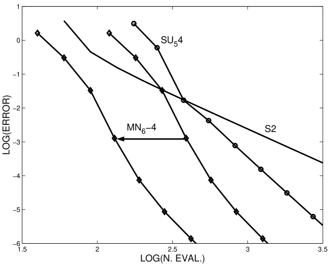
Figure 20: Average error versus number of force evaluations in the numerical integration of (326) using second and fourth order symplectic integrators for general separable systems (S2 corresponds to the second order leapfrog method with coefficients (327) and SU${}_{5}4$ to the fourth order method with coefficients (328)) and the fourth order symplectic Runge–Kutta–Nyström method MN${}_{6}4$ with initial conditions $q(0)=1.75$, $p(0)=0$ and $\epsilon=1/20$, $\delta=1/4$, $\omega=1$.

6 Some applications of the numerical integrators based on ME

In this section we collect several examples where the numerical integration methods based on the Magnus expansion have been applied in the recent literature. Special attention is dedicated to the numerical integration of the Schrödinger equation, since the Magnus series expansion has been extensively used in this setting almost since its very formulation. The time-independent Schrödinger equation can be considered as a particular example of a Sturm–Liouville problem, so we also review the applicability of Magnus based techniques in this context. Then we consider a particular nonlinear system (the differential Riccati equation) which can be, in some sense, linearized, so that at the end one may work with finite-dimensional matrices. Finally, we summarize a recent but noteworthy application: the design of new classes of numerical schemes for the integration of stochastic differential equations.

6.1 Case study: numerical treatment of the Schrödinger equation

Before embarking ourselves in the use of numerical methods based on the Magnus expansion in the integration of the Schrödinger equation, let us establish first the theoretical framework which allows one to use numerical integrators in this setting for obtaining approximate solutions in time and space.

6.1.1 Time-dependent Schrödinger equation

To keep the treatment as simple as possible, we commence by considering the one-dimensional time-dependent Schrödinger equation ($\hbar=1$)

$$i\frac{\partial}{\partial t}\psi(t,x)=H\psi(t,x)\equiv-\frac{1}{2}\frac{\partial^{2}}{\partial x^{2}}\psi(t,x)+V(x)\psi(t,x),$$ (329)

with initial condition $\psi(0,x)=\psi_{0}(x)$. If we look for a solution of the form $\psi(t,x)=\phi(t)\,\varphi(x)$, it is clear that, by substituting into (329), one gets $\phi(t)=\e^{-itE}$, where $E$ is a constant and $\varphi(x)$ is the solution of the second order differential equation

$$-\frac{d^{2}\varphi}{dx^{2}}+V(x)\varphi=E\varphi.$$ (330)

If $E>V$ the solution is oscillatory, whereas if $E<V$ the solution is a linear combination of exponentially increasing and decreasing functions. For bounded problems this last condition always takes place at the boundaries. Since

$$\int|\psi(x,t)|^{2}dx=\int|\varphi(x)|^{2}dx<\infty,$$ (331)

it is clear that the exponentially increasing solutions have to be cancelled, and this can only occur for certain values of the constant $E$, which are precisely the eigenvalues of the problem.

Let us assume that the system has only a discrete spectrum and denote by $\{E_{n},\varphi_{n}\}_{n=0}^{\infty}$, with $E_{i}<E_{j},\ i<j$, the complete set of eigenvalues and associated eigenvectors. It is well known that we can take $\{\varphi_{n}\}_{n=0}^{\infty}$ as an orthonormal basis and, since (329) is linear, any solution can be written as

$$\psi(t,x)=\sum_{n=0}^{\infty}c_{n}\,\e^{-itE_{n}}\varphi_{n}(x).$$ (332)

Using the standard notation for the inner product, one has

$$\langle\varphi_{n}(x)|\psi(t,x)\rangle=\int\varphi_{n}^{*}(x)\,\psi(t,x)dx=c_{n}\,\e^{-itE_{n}}$$ (333)

and

$$|\langle\varphi_{n}(x)|\psi(t,x)\rangle|^{2}=|c_{n}|^{2}$$

is the probability to find the system in the eigenstate $\varphi_{n}$, so that $\sum_{n}|c_{n}|^{2}=1$. The energy is given by

$$\mathcal{E}=\langle\psi|H|\psi\rangle=\int\psi^{*}(t,x)\,H\,\psi(t,x)dx=\sum_{n=1}^{\infty}\sum_{m=1}^{\infty}c_{n}^{*}c_{m}H_{n,m},$$ (334)

where

$$H_{n,m}\equiv\langle m|H|n\rangle=\langle\varphi_{m}|H|\varphi_{n}\rangle.$$

In general, the coefficients $c_{n}$ decrease very fast with $n$ and, in some cases, the system allows only a finite number of states. In that situation, one may consider the Schrödinger equation as a finite dimensional linear system where the Hamiltonian is a matrix with elements $H_{n,m}$. This is precisely the case for the examples examined in section 4.

When the Hamiltonian is explicitly time-dependent, this procedure is not longer valid. Instead one may use some alternative techniques which we now briefly review.

(i) Spectral Decomposition. Let us assume that the system is perturbed with a time-dependent potential, i.e., equation (329) takes the form

$$i\frac{\partial}{\partial t}\psi(t,x)=\hat{H}(t)\psi(t,x)\equiv(\hat{T}+\hat{V}(t))\,\psi(t,x),$$ (335)

where

$$\hat{T}\psi\equiv-\frac{1}{2}\frac{\partial^{2}\psi}{\partial x^{2}},\qquad\hat{V}(t)\psi\equiv(V(x)+\tilde{V}(t,x))\,\psi.$$

In this case we cannot use separation of variables. However, since $\{\varphi_{n}\}$ is a complete bases we can still write the solution as

$$\psi(t,x)\simeq\sum_{n=0}^{d-1}c_{n}(t)\,\e^{-itE_{n}}\,\varphi_{n}(x),$$ (336)

where $E_{n}$ and $\varphi_{n}$ are the exact eigenvalues and eigenfunctions when $\tilde{V}=0$, and the complex coefficients $c_{n}$ give the probability amplitude to find the system in the state $\varphi_{n}$ ($\sum_{n}|c_{n}(t)|^{2}=1$ for all $t$). Then, substituting (336) into (335) we obtain the matrix equation

$$i\,\frac{d}{dt}{\bf c}(t)={\bf H}(t){\bf c}(t),\qquad\qquad{\bf c}(0)={\bf c}_{0},$$ (337)

where $\ {\bf c}=(c_{0},\ldots,c_{d-1})^{T}\in\mathbb{C}^{d}\$ and $\,{\bf H}\in\mathbb{C}^{d\times d}\,$ is an Hermitian matrix associated to the Hamiltonian

$$\,({\bf H}(t))_{ij}=\langle\varphi_{i}|\hat{H}(t)-\hat{H}_{0}|\varphi_{j}\rangle\,\e^{i(E_{i}-E_{j})t},\qquad i,j=1,\ldots,d$$

and $\hat{H}_{0}=\hat{H}(t=0)$. Given the initial wave function $\psi(0,x)$, the components of ${\bf c}_{0}$ are determined by $c_{0,i}=\langle\varphi_{i}|\psi(0,x)\rangle$.

Obviously, any complete basis can be used in this case, although the norm of the matrix ${\bf H}(t)$ may depend on the choice. In addition, the number of basis elements, i.e. the minimum dimension $d$ necessary to obtain a sufficiently accurate result, also depends on the chosen basis.

(ii) Space discretization. This procedure intends to take profit of the structure of the Hamiltonian $\hat{H}$ in (335): $\hat{V}$ is diagonal in the coordinate space and $\,\hat{T}\,$ is diagonal in the momentum space. Let us assume that the system is defined in the interval $\,x\in[x_{0},x_{f}]$ with periodic boundary conditions. We can then split this interval in $d$ parts of length $\Delta x=(x_{f}-x_{0})/d\,$ and consider $\,c_{n}=\psi(t,x_{n})\,$ where $x_{n}=x_{0}+n\Delta x,$ $n=0,1,\ldots,d-1$. Then a finite dimensional linear equation similar (but with a different coefficient matrix $\mathbf{H}$) to equation (337) results. Since $\,\hat{V}$ is diagonal in the coordinate space and $\,\hat{T}\,$ is diagonal in momentum space, it is possible to use complex Fast Fourier Transforms (FFTs) for evaluating the products ${\bf H}{\bf c}$, where $\,\hat{T}\psi(t,x_{n})=\mathcal{F}^{-1}D_{T}\mathcal{F}\psi(t,x_{n})$, and $\,D_{T}\,$ is a diagonal operator.

We thus see that whatever the procedure used (spectral decomposition or space discretization), one ends up with a linear equation of the form

$$i\frac{d\psi}{dt}(t)=H(t)\psi(t),\qquad\psi(0)=\psi_{0}$$ (338)

where now $\psi(t)$ represents a complex vector with $d$ components which approximates the (continuous) wave function. The computational Hamiltonian $H(t)$ appearing in (338) is thus a space discretization (or other finite-dimensional model) of $\hat{H}(t)=\hat{T}+\hat{V}(t)$. Numerical difficulties come mainly from the unbounded nature of the Hamiltonian and the highly oscillatory behaviour of the wave function.

It is at this point when numerical algorithms based on the Magnus expansion, such as they have been formulated in previous sections, come into play for integrating in time the linear system (338). To put them in perspective, let us introduce first some other numerical methods also used in this context. Our exposition is largely based on the reference [156].

The implicit midpoint rule

The approximation to the solution of (338) provided by this scheme is implicitly defined by

$$i\frac{\psi_{n+1}-\psi_{n}}{\Delta t}=H(t_{n+1/2})\,\frac{1}{2}(\psi_{n+1}+\psi_{n}),$$ (339)

where $t_{n+1/2}=\frac{1}{2}(t_{n+1}+t_{n})$. Here and in the sequel, for clarity, we have denoted by $\Delta t$ the time step size and $t_{n}=n\Delta t$. Alternatively,

$$\psi_{n+1}=r(-i\Delta tH(t_{n+1/2}))\,\psi_{n},\quad\mbox{ with }\quad r(z)=\frac{1+\frac{1}{2}z}{1-\frac{1}{2}z}.$$ (340)

Observe that, as $r$ is nothing but the Cayley transform, the numerical propagator is unitary and consequently the Euclidean norm of the discrete wave function is preserved along the evolution: $\|\psi_{n+1}\|=\|\psi_{n}\|$. This is a crucial qualitative feature the method shares with the exact solution, contrarily to other standard numerical integrators, such as explicit Runge–Kutta methods. From a purely numerical point of view, the algorithm is stable for any step size $\Delta t$.

Another useful property of this numerical scheme is time-symmetry: exchanging in (340) $n$ by $n+1$ and $\Delta t$ by $-\Delta t$ we get the same numerical method again. Equivalently, $r(-z)=r(z)^{-1}$, exactly as the exponential $\e^{z}$.

With respect to accuracy, it is not difficult to show that, if $H(t)$ is bounded and sufficiently smooth, the error verifies

$$\|\psi_{n}-\psi(t_{n})\|=\mathcal{O}(\Delta t^{2})$$ (341)

uniformly for $n\Delta t$ in a time interval $[0,t_{f}]$. In other words, the implicit midpoint rule is a second-order method. It happens, however, that the constant in the term $\mathcal{O}(\Delta t^{2})$ depends on bounds of $H^{\prime}$ and $H^{\prime\prime}$ and on the norm of the third derivative of the solution $\psi$. Since, in general, the wave function is highly oscillatory in time, this time derivative can become large, and so the use of very small time steps is mandatory.

The exponential midpoint rule

Another possibility to get approximate solutions of (338) consists in replacing $r(z)$ by $\exp(z)$ in (340):

$$\psi_{n+1}=\exp(-i\Delta t\,H(t_{n+1/2}))\,\psi_{n}.$$ (342)

Now, instead of solving systems of linear equations as previously, one has to compute the exponential of a large matrix times a vector at each integration step. In this respect, the techniques reviewed in subsection 5.6 can be efficiently implemented. The exponential midpoint rule (342) also provides a unitary propagator and it is time-symmetric. In addition, the error satisfies the same condition (341), but now the constant in the $\mathcal{O}(\Delta t^{2})$ term is independent of the time derivatives of $\psi$ under certain assumptions on the commutator $[H(t),H(s)]$ [104]. As a consequence, much larger time steps can be taken to achieve the same accuracy as with the implicit midpoint rule.

Integrators based on the Magnus expansion

The method (342) is a particular instance of a second order Magnus method when the integral $\int_{0}^{\Delta t}H(s)ds$ is replaced by the midpoint quadrature rule. In fact, we have already used it in (292). Obviously, if higher order approximations are considered, the accuracy can be enhanced a great deal. This claim has to be conveniently justified, however, since the order of the numerical methods based on Magnus has been deduced when $\|\Delta tH(t)\|\rightarrow 0$ and is obtained by studying the remainder of the truncated Magnus series. In the Schrödinger equation, on the other hand, one has to cope with discretizations of unbounded operators, so in principle it is not evident how the previous results on the order of accuracy apply in this context. In [104], Hochbruck and Lubich analyse in detail the application of the fourth-order Magnus integrator (271) to equation (338), showing that it works extremely well even with step sizes for which the corresponding $\|\Delta tH(t)\|$ is large. In particular, the scheme retains fourth order of accuracy in $\Delta t$ independently of the norm of $H(t)$ when $H(t)=T+V(t)$, $T$ is a discretization of $-\frac{1}{2}\frac{\partial^{2}}{\partial x^{2}}$ (with maximum eigenvalue $E_{\mathrm{max}}\sim(\Delta x)^{-2}$) and $V(t)$ is sufficiently smooth under the time step restriction $\Delta t\sqrt{E_{\mathrm{max}}}\leq Const.$ This is so even when there is no guarantee that the Magnus series converges at all.

Symplectic perspective

The evolution operator corresponding to (335) is not only unitary, but also symplectic with canonical coordinates and momenta $\mbox{Re}(\psi)$ and $\mbox{Im}(\psi)$, respectively. If we carry out a discretization in space, this symplectic structure is inherited by the corresponding equation (337). It makes sense, then, to write ${\bf c}={\bf q}+i{\bf p}$ and consider the equations satisfied by ${\bf q,p}\in\mathbb{R}^{d}$, namely

$$\mathbf{q}^{\prime}=\mathbf{H}(t)\mathbf{p},\qquad\mathbf{p}^{\prime}=-\mathbf{H}(t)\mathbf{q},$$ (343)

which can be interpreted as the canonical equations corresponding to the Hamiltonian [95]

$$\mathcal{H}(t,{\bf q,p})={\bf p}^{T}{\bf H}(t){\bf p}+{\bf q}^{T}{\bf H}(t){\bf q}.$$ (344)

Denoting ${\bf z=(q,p)}^{T}$, it is clear that

$${\bf z}^{\prime}=\left({\bf A}(t)+{\bf B}(t)\right)\,{\bf z}$$

where

$${\bf A}(t)=\left(\begin{array}[]{cc}0&\;\;{\bf H}(t)\\ 0&0\end{array}\right),\qquad\quad{\bf B}(t)=\left(\begin{array}[]{cr}0&\;\;0\\ -{\bf H}(t)&0\end{array}\right).$$ (345)

For this system it is possible, therefore, to apply the commutator-free Magnus integrators constructed in subsection 5.8.2. In addition, one has

$${\bf[B,[B,[B,A]]]=[A,[A,[A,B]]]=0},$$

and this property allows us to use especially designed and highly efficient integration methods [20].

6.1.2 Time-independent Schrödinger equation

Restricting ourselves to the time-independent Schrödinger equation (330), we next illustrate how Magnus integrators can in fact be used to compute the discrete eigenvalues defined by the problem. Although only the Schrödinger equation in a finite domain is considered,

$$-\frac{d^{2}\varphi}{dx^{2}}+V(x)\varphi=\lambda\varphi,\qquad x\in(a,b)$$ (346)

the procedure can be easily adapted to other types of eigenvalue problems, in which one has to find both $\lambda\equiv E$ and $\varphi$. Here it is assumed that the potential is smooth, $V\in C^{m}(a,b)$ and, for simplicity, $\varphi(a)=\varphi(b)=0$.

Under these assumptions, it is well known that the eigenvalues are real, distinct and bounded from below. The problem (346) can be formulated in the special linear group $\mathrm{SL}(2)$,

$$\frac{d\mathbf{y}}{dx}=\left(\begin{array}[]{ccr}0&&\ \ 1\\ V(x)-\lambda&&0\end{array}\right)\mathbf{y},\qquad x\in(a,b),\qquad\mbox{ where }\quad\mathbf{y}=(\varphi,d\varphi/dx)^{T},$$ (347)

so that the Magnus expansion can be applied in a natural way. As usual, rather than approximating the fundamental solution of (347) in the entire interval $(a,b)$ by $\exp(\Omega)$, the idea is to partition the interval into $N$ small subintervals, and then apply a conveniently discretized version of the Magnus expansion. In this way, the convergence problem no longer restricts the size $(b-a)$ [172].

For the sake of simplicity, let us consider the fourth-order method (271). Writing

$$V_{n,1}=V(x_{n}+(\frac{1}{2}-\frac{\sqrt{3}}{6})h),\qquad V_{n,2}=V(x_{n}+(\frac{1}{2}+\frac{\sqrt{3}}{6})h),$$

where $h=(b-a)/N$ and $x_{n}=a+h\,n$, we form

$$\sigma_{n}(\lambda)=\left(\begin{array}[]{ccc}-\frac{\sqrt{3}}{12}h^{2}(V_{n,1}-V_{n,2})&&\ \ \ h\\ \frac{1}{2}h(V_{n,1}+V_{n,2})-h\lambda&&\frac{\sqrt{3}}{12}h^{2}(V_{n,1}-V_{n,2})\end{array}\right),$$

for $n=0,1,\ldots,N-1$. Then, the fourth-order approximation to the solution of (347) at $x=b$ is

$$\mathbf{y}(b)=\e^{\sigma_{N-1}(\lambda)}\cdots\e^{\sigma_{1}(\lambda)}\,\e^{\sigma_{0}(\lambda)}\mathbf{y}(a)$$ (348)

and the values of $\lambda$ are obtained from (348) by using repeatedly the expression of the exponential of a traceless matrix, eq. (24), and requiring that $\varphi(a)=\varphi(b)=0$. The resulting nonlinear equation in $\lambda$ can be solved, for instance, by Newton–Raphson iteration, which provides quadratic convergence for starting values sufficiently near the solution [172].

Although by construction this procedure leads to a global order of approximation $\mathcal{O}(h^{p})$ if a $p$th-order Magnus method is applied, it turns out that the error also depends on the magnitude of the eigenvalue. Specifically, the error in a $p$th-order method grows as $\mathcal{O}(h^{p+1}\lambda^{p/2-1})$ [172], and thus one expects poor approximations for large eigenvalues. This difficulty can be overcome up to a point by analyzing the dependence on $\lambda$ of each term in the Magnus series and considering partial sums of the terms carrying the most significant dependence on $\lambda$. For instance, it is possible to design a sixth-order Magnus integrator for this problem with error $\mathcal{O}(h^{7}\lambda)$, which therefore behaves like a fourth-order method when $h^{2}\lambda\approx 1$, whereas the standard sixth-order Magnus scheme, carrying an error of $\mathcal{O}(h^{7}\lambda^{2})$, reduces to an order-two method [172]. In any case, getting accurate approximations when $|\lambda|\rightarrow\infty$ is more problematic [128].

6.2 Sturm–Liouville problems

The system defined by (346) with boundary conditions $\varphi(a)=\varphi(b)=0$ is just one particular example of a second order Sturm–Liouville problem [199, 246]. It is thus quite natural to try to apply Magnus integrators to more general problems within this class.

A second order Sturm–Liouville eigenvalue problem has the form

$$\frac{d}{dx}\left(p(x)\frac{dy}{dx}(x)\right)+q(x)y(x)=\lambda\,r(x)y(x)\qquad\mbox{ on }(a,b)$$ (349)

with separated boundary conditions which commonly have the form

$$A_{1}y(a)+A_{2}p(a)y^{\prime}(a)=0\qquad B_{1}y(b)+B_{2}p(b)y^{\prime}(b)=0$$ (350)

for given constants $A_{i},B_{i}$ and functions $p(x)$, $q(x)$ and $r(x)$. Solving this problem means, of course, determining the values $\lambda_{n}$ of $\lambda$ for which eq. (349) has a nontrivial (continuously differentiable square integrable) solution $y_{n}(x)$ satisfying equations (350) [246, 7].

These and other higher order Sturm–Liouville problems can be recasted as a linear matrix system of the form

$$Y^{\prime}=(\lambda B+C(x))\,Y$$ (351)

by transforming to the so-called compound matrix or modified Riccati variables [96, 128]. Here $B$ is a constant matrix. When generalizing the above treatment based on the Magnus expansion to this problem, there is one elementary but important remark worth to be stated explicitly: unless the differential equation (351) has the same large $\lambda$-asymptotics as some differential equation with $x$-independent coefficients, then it will be impossible to develop a Magnus method which accurately approximate its solutions for large $\lambda$ [128]. The reason is that a Magnus method approximates the solution by a discrete solution calculated using a formula of the form $Y(x_{n+1})=\exp(\sigma_{n}(\lambda))Y(x_{n})$; in particular, on the first step $(x_{0},x_{1})$, the differential equation is approximated by one in which the coefficient matrix is replaced by the $x$-independent matrix $\sigma_{0}(\lambda)/(x_{1}-x_{0})$.

In consequence, the attention should be restricted to systems for which it is known that a suitable constant-coefficient system provides the correct asymptotics. This is the case, in particular, for equation (346), and more generally for linear equations of order $2n$ in which the $(2n-1)$st derivative is zero, such as

$$(-1)^{n}y^{(2n)}+\sum_{j=0}^{2n-2}q_{j}(x)y^{(j)}=\lambda y.$$

Here the asymptotics are determined by the equation $(-1)^{n}y^{(2n)}=\lambda y$ [187]. Even then, the methods developed in [172] for equation (346) and implemented for systems with matrices of general size in [128] require a $\lambda$-dependent step size restriction of the form $h\leq\mathcal{O}(|\lambda|^{-1/4})$ in order to be defined. Nevertheless, the analysis carried out in [128] shows that the fourth order Magnus integrator based on a two-point Gaussian quadrature appears to offer significant advantages over conventional methods based on power series and library routines.

Magnus integrators have also been successfully applied in the somewhat related problem of computing the Evans function for spectral problems arising in the analysis of the linear stability of travelling wave solutions to reaction-diffusion PDEs [5]. In this setting, Magnus integrators possess some appealing features in comparison, for instance, with Runge–Kutta schemes: (1) they are unconditionally stable; (2) their performance is superior in highly oscillatory regimes and (3) their step size can be controlled in advance. Items (2) and (3) are due to the fact that error bounds for Magnus methods depend only on low order derivatives of the coefficient matrix, not (as for Runge–Kutta schemes) on derivatives of the solution. Therefore, performance and, correspondingly, the choice of optimal step size remain uniform over any bounded region of parameter space [5].

6.3 The differential Riccati equation

Let us consider now the two-point boundary value problem in the $t$ variable defined by the linear differential equation

$${\bf y}^{\prime}\equiv\left(\begin{array}[]{c}{\bf y}_{1}^{\prime}\\ {\bf y}_{2}^{\prime}\end{array}\right)=\left(\begin{array}[]{cc}A(t)&\ \ B(t)\\ C(t)&D(t)\end{array}\right)\ \left(\begin{array}[]{c}{\bf y}_{1}\\ {\bf y}_{2}\end{array}\right),\qquad 0<t<T$$ (352)

with separated boundary conditions

$$(K_{11}\;\;K_{12})\left(\begin{array}[]{c}{\bf y}_{1}\\ {\bf y}_{2}\end{array}\right)_{t=0}=\;\gamma_{1},\qquad(K_{21}\;\;K_{22})\left(\begin{array}[]{c}{\bf y}_{1}\\ {\bf y}_{2}\end{array}\right)_{t=T}=\,\gamma_{2}.$$ (353)

Here $A\in\mathbb{C}^{q\times q}\,$, $B\in\mathbb{C}^{q\times p}$, $C\in\mathbb{C}^{p\times q}\,$, $D\in\mathbb{C}^{p\times p}\,$, whereas ${\bf y}_{1},\gamma_{2}\in\mathbb{C}^{p}$, ${\bf y}_{2},\gamma_{1}\in\mathbb{C}^{q}$ and the matrices $K_{ij}$ have appropriate dimensions. We next introduce the time-dependent change of variables (or picture) ${\bf y}=Y_{0}(t)\,{\bf w}$, with

$$Y_{0}(t)=\left(\begin{array}[]{cc}I_{p}&\ \ 0\\ X(t)&I_{q}\end{array}\right)$$ (354)

and choose the matrix $X\in\mathbb{C}^{p\times q}$ so as to ensure that in the new variables $\mathbf{w}=Y_{0}^{-1}(t)\mathbf{y}$ the system assume the partly decoupled structure [63]

$${\bf w}^{\prime}\equiv\left(\begin{array}[]{c}{\bf w}_{1}^{\prime}\\ {\bf w}_{2}^{\prime}\end{array}\right)=\left(\begin{array}[]{cc}A+BX&\ \ B\\ O&D-XB\end{array}\right)\ \left(\begin{array}[]{c}{\bf w}_{1}\\ {\bf w}_{2}\end{array}\right),$$ (355)

together with the corresponding boundary conditions for ${\bf w}$. It turns out that this is possible if and only if $X(t)$ satisfies the so-called differential Riccati equation [64]

$$X^{\prime}=C(t)+D(t)X-XA(t)-XB(t)X,\qquad X(0)=X_{0}$$ (356)

for some $X_{0}$. By requiring

$$X_{0}=-K_{12}^{-1}K_{11},$$ (357)

then the boundary conditions (353) also decouple as

$$(O\;\;K_{12}){\bf w}(0)=\gamma_{1},\qquad\big{(}K_{21}+K_{22}X(T)\;\;\;K_{22}\big{)}{\bf w}(T)=\gamma_{2}.$$ (358)

Here we assume without loss of generality that $K_{12}$ is invertible. In this way, the original boundary value problem can be solved as follows [63, 64]: (i) solve equation (356) with initial condition (357) from $t=0$ to $t=T$; (ii) solve the $\mathbf{w}_{2}$-equation in (355) and (358), also from zero to $T$; (iii) solve the $\mathbf{w}_{1}$-equation in (355) from $t=T$ to $t=0$ and recover ${\bf y}=Y_{0}(t)\,{\bf w}$. In other words, the solution of the original two-point boundary value problem can be obtained by solving a sequence of three different initial value problems, one of which involves the nonlinear equation (356). Obviously, steps (i) and (iii) can be solved using numerical integrators based on the Magnus expansion. It could be perhaps more surprising that these algorithms can indeed be used to integrate the Riccati equation in step (ii).

Although the boundary value problem (352) is a convenient way to introduce the differential Riccati equation (356), this equation arises in many fields of science and engineering, such as linear quadratic optimal control, stability theory, stochastic control, differential games, etc. Accordingly, it has received considerable attention in the literature, both focused to its theoretical aspects [17, 200] and its numerical treatment [63, 133, 211].

In order to apply Magnus methods to solve numerically the Riccati equation, we first apply the transformation

$$X(t)\ =\ V(t)\,W^{-1}(t),$$ (359)

with $V\in\mathbb{C}^{p\times q}$, $W\in\mathbb{C}^{q\times q}$ and $V(0)=X_{0},W(0)=I_{q}$, in the region where $W(t)$ is invertible. Then eq. (356) is equivalent to the linear system

$$\begin{array}[]{c}\displaystyle Y^{\prime}\,=\,S(t)\,Y(t)\,,\qquad Y(0)\,=\,\left(\begin{array}[]{c}I_{q}\\ X_{0}\end{array}\right)\end{array}$$ (360)

with

$$\begin{array}[]{c}\displaystyle Y(t)=\left(\begin{array}[]{c}W(t)\\ V(t)\end{array}\right),\qquad\qquad S(t)=\left(\begin{array}[]{cc}A(t)&\ \ B(t)\\ C(t)&D(t)\end{array}\right)\end{array}$$ (361)

so that the previous Magnus integrators for linear problems can be applied here. Apparently, this system is similar to (352), but now we are dealing with an initial value problem and $Y$ is a matrix instead of a vector.

When dealing in general with the differential Riccati equation (356), it is meaningful to distinguish the following three cases:

• The so-called symmetric Riccati equation, which corresponds to $q=p$, $D(t)=-A(t)^{T}$ real, and $B(t)$, $C(t)$ real and symmetric matrices. In this case, the solution satisfies $X^{T}=X$. It is straightforward to show that this problem is equivalent to the treatment of the generalized time-dependent harmonic oscillator, described by the Hamiltonian function

  $$H=\frac{1}{2}{\bf p}^{T}B(t){\bf p}+{\bf p}^{T}A(t){\bf q}-\frac{1}{2}{\bf q}^{T}C(t){\bf q}.$$

  The approximate solution attained by Magnus integrators when applied to (360)-(361) can be seen as the exact solution corresponding to a perturbed symplectic matrix $\tilde{S}(t)\simeq S(t)$. In other words, we are solving exactly a perturbed Hamiltonian system so that the approximate solution, $\tilde{X}$, will shares several properties of the exact solution, in particular $\tilde{X}^{T}=\tilde{X}$.

• The linear non-homogeneous problem

  $$X^{\prime}=D(t)X+C(t)$$ (362)

  corresponds to the particular case $A=0$ and $B=0$ in (356).

• The problem

  $$X^{\prime}=D(t)X+XA(t)$$ (363)

  is recovered from (356) by taking $C=0$ and $B=0$. It has been treated in [112] by developing an ad hoc Magnus-type expansion. Notice that the case $p=q$, $D=-A$ corresponds to the linear isospectral system (255).

6.4 Stochastic differential equations

In recent years the use of stochastic differential equations (SDEs) has become widespread in the simulation of random phenomena appearing in physics, engineering, economics, etc, such as turbulent diffusion, polymer dynamics and investment finance [35]. Although models based on SDEs can offer a more realistic representation of the system than ordinary differential equations, the design of effective numerical schemes for solving SDEs is, in comparison with ODEs, a less developed field of research. This fact notwithstanding, it is true that recently new classes of integration methods have been constructed which automatically incorporate conservation properties the SDE possesses. Since some of the methods are based precisely on the Magnus expansion, we briefly review here their main features, and refer the reader to the more advanced literature on the subject [35, 141, 196].

A SDE in its general form is usually written as

$$dy(t)=g_{0}(t,y(t))\,dt+\sum_{j=1}^{d}g_{j}(t,y(t))\,dW_{j}(t),\qquad y(0)=y_{0},\qquad y\in\mathbb{R}^{m},$$ (364)

where $g_{j}$, ($j\geq 0$), are $m$-vector-valued functions. The function $g_{0}$ is the deterministic continuous component (called the drift coefficient), the $g_{j}$, ($j\geq 1$), represent the stochastic continuous components (the diffusion coefficients) and $W_{j}$ are $d$ independent Wiener processes. A Wiener process $W$ (also called Brownian motion) is a stochastic process [35] satisfying

$$W(0)=0,\qquad E[W(t)]=0,\qquad\mathrm{Var}[W(t)-W(s)]=t-s,\quad t>s$$

which has independent increments on non-overlapping intervals. In other words, a Wiener process is normally distributed with mean or expectation value $E$ equal to zero and variance $t$.

Equation (364) can be written in integral form as

$$y(t)=y_{0}+\int_{0}^{t}g_{0}(s,y(s))\,ds+\sum_{j=1}^{d}\int_{0}^{t}g_{j}(s,y(s))\,dW_{j}(s).$$ (365)

The $d$ integrals in (365) cannot be considered as Riemann–Stieltjes integrals, since the sample paths of a Wiener process are not of bounded variation. In fact, if different choices are made for the point $\tau_{i}$ (in the subintervals $[t_{i-1},t_{i}]$ of a given partition) where the function is evaluated, then the approximating sums for each $g_{j}$,

$$\sum_{i=1}^{N}g_{j}(\tau_{i},y(\tau_{i}))(W_{j}(t_{i})-W_{j}(t_{i-1})),\qquad\tau_{i}=\theta t_{i}+(1-\theta)t_{i-1},$$ (366)

converge (in the mean-square sense) to different values of the integral, depending on the value of $\theta$ [34]. Thus, for instance,

$$\int_{a}^{b}W(t)dW(t)=\frac{1}{2}(W^{2}(b)-W^{2}(a))+(\theta-\frac{1}{2})(b-a).$$

If $\theta=0$, then $\tau_{i}=t_{i-1}$ (the left-hand point of each subinterval) and the resulting integral is called an Itô integral; if $\theta=1/2$ (so that the midpoint is used instead), one has a Stratonovich integral. These are the two main choices and, although they are related, the particular election depends ultimately on the nature of the process to be modeled [34]. It can be shown that the Stratonovich calculus satisfies the Riemann–Stieltjes rules of calculus, and thus it is the natural choice here.

When dealing with numerical methods for solving (364), there are two ways of measuring accuracy [35]. The first is strong convergence, essential when the aim is to get numerical approximations to the trajectories which are close to the exact solution. The second is weak convergence, when only certain moments of the solution are of interest. Thus, if $\hat{y}_{n}$ denotes the numerical approximation to $y(t_{n})$ after $n$ steps with constant step size $h=(t_{n}-t_{0})/n$, then the numerical solution $\hat{y}$ converges strongly to the exact solution $y$ with strong global order $p$ if there exist $C>0$ (independent of $h$) and $\delta>0$ such that

$$E[\|\hat{y}_{n}-y(t_{n})\|]\leq Ch^{p},\qquad h\in(0,\delta).$$

It is worth noticing that $p$ can be fractional, since the root mean-square order of the Wiener process is $h^{1/2}$. One of the simplest procedures for solving (364) numerically is the so-called Euler–Maruyama method [164],

$$y_{n+1}=y_{n}+\sum_{j=0}^{d}J_{j}g_{j}(t_{n},y_{n}),$$ (367)

where

$$h=t_{n+1}-t_{n},\quad J_{0}=h,\quad J_{j}=W_{j}(t_{n+1})-W_{j}(t_{n}),\quad j=1,\ldots,d.$$

This scheme turns out to be of strong order $1/2$. Here the $J_{j}$ can be computed as $\sqrt{h}N_{j}$, where the $N_{j}$ are $N(0,1)$ normally distributed independent random variables [34].

For the general non-autonomous linear Stratonovich problem defined by

$$dy=G_{0}(t)y\,dt+\sum_{j=1}^{d}G_{j}(t)\,y\,dW_{j},\qquad y(0)=y_{0}\in\mathbb{R}^{m}$$ (368)

the Magnus expansion for the deterministic case can be extended in a quite straightforward way. It is well worth noticing that in equation (368), even when the functions $G_{j}$ are constant, there is no explicit solution [141], unless all the $G_{j}$, $j\geq 0$, commute with one another, in which case it holds that

$$y(t)=\exp\left(G_{0}\,t+\sum_{j=1}^{d}G_{j}W_{j}(t)\right)y_{0}.$$ (369)

In many modeling situations, however, there is no reason to expect that the functions $G_{j}$ associated with the Wiener processes commute. If for simplicity we only consider the autonomous case and write

$$G(t)\equiv G_{0}\,dt+\sum_{j=1}^{d}G_{j}\,dW_{j}(t),$$

then (368) can be expressed as

$$dy=G(t)\,y\,dt,\qquad y(0)=y_{0}$$

and thus one can formally apply the Magnus expansion to this equation to get $y(t)=\exp(\Omega(t))y_{0}$. The first term in the series reads in this case

$$\int_{0}^{t}G(s)\,ds\equiv\int_{0}^{t}G_{0}\,ds+\sum_{j=1}^{d}\int_{0}^{t}G_{j}\,dW_{j}(s)=G_{0}\,t+\sum_{j=1}^{d}G_{j}J_{j},$$

where now

$$J_{j}=\int_{0}^{t}dW(s)=W_{j}(t)-W_{j}(0).$$

By inserting these expressions into the recurrence associated with the Magnus series, Burrage and Burrage [34] show that

$$\Omega(t) = \sum_{j=0}^{d}G_{j}J_{j}+\frac{1}{2}\sum_{i=0}^{d}\sum_{j=i+1}^{d}[G_{i},G_{j}](J_{ji}-J_{ij})$$

$$+\sum_{i=0}^{d}\sum_{k=0}^{d}\sum_{j=k+1}^{d}[G_{i},[G_{j},G_{k}]]\left(\frac{1}{3}(J_{kji}-J_{jki})+\frac{1}{12}J_{i}(J_{jk}-J_{kj})\right)+\cdots,$$

where the multiple Stratonovich integrals are defined by

$$J_{j_{1}j_{2}\cdots j_{l}}(t)=\int_{0}^{t}\int_{0}^{s_{l}}\cdots\int_{0}^{s_{2}}dW_{j_{1}}(s_{1})\cdots dW_{j_{l}}(s_{l}),\qquad j_{i}\in\{0,1,\ldots,d\}.$$ (371)

Since not all the Stratonovich integrals are independent, one has to compute only $d(d+1)(d+5)/6$ stochastic integral evaluations to achieve strong order 1.5 with the expression (6.4) [34]. If, on the other hand, $\Omega(t)$ is truncated after the first set of terms, then the resulting numerical approximation

$$y(t)=\exp\left(\sum_{j=0}^{d}G_{j}J_{j}\right)y_{0}$$

has strong order $1/2$, but leads to smaller error coefficients than the Euler–Maruyama method (367) [34]. Furthermore, the error becomes smaller as the $G_{i}G_{j}$ terms get closer to commuting and the scheme preserves the underlying structure of the problem.

One should notice at this point that equation (364) (or, in the linear case, equation (368)), has formally the same structure as the nonlinear ODE (171) appearing in control theory. Therefore, the formalism developed there to get the Chen–Fliess series can be applied here with the alphabet $I=\{0,1,\ldots,d\}$ and the integrals

$$\left(\int_{0}\mu\right)(t)=\int_{0}^{t}\mu(s)\,ds,\qquad\left(\int_{i}\mu\right)(t)=\int_{0}^{t}\mu(s)\,dW_{i}(s),\quad i\geq 1,$$

since the Stratonovich integrals satisfy the integration by parts rule. In other words, one can obtain the corresponding Magnus expansion for arbitrary (linear or nonlinear) stochastic differential equations simply by following the same procedure as for deterministic ODEs.

With respect to nonlinear Stratonovich stochastic differential equations, it should be remarked that the use of Lie algebraic techniques as well as the design of Lie group methods for obtaining strong approximations when the solution evolves on a smooth manifold has received considerable attention in the recent literature [150, 161, 170].

7 Physical applications

From previous sections it should be clear that ME has a strong bearing on both Classical and Quantum Mechanics. As far as Classical Mechanics is concerned this has been most explicitly shown in section 3.4. On its turn Quantum Mechanics has been repeatedly invoked as a source of applications, among others, in sections 2.9 and 4. In this section we present in a very schematic way and with no aim at completeness some applications of ME in different areas of the physical sciences. This will show that over the years ME has been one of the preferred options to deal with equation (4) which, under different appearances, pervades the entire field of Physics. In the works mentioned here, almost exclusively analytical methods are used and, in general, one must recognize that in most, if not all, cases listed only the first two orders of the expansion have been considered. In very specially simple applications, due to particular algebraic properties of the operators involved, this happens to be exact. Only with the more recent advent of the numerical applications, as has been emphasized in sections 5 and 6, has the expansion been carried in a more systematic way to higher orders.

7.1 Nuclear, atomic and molecular physics

As far as we know the first physical application of ME dates back to 1963. Robinson [203] published a brand new formalism to investigate multiple Coulomb excitations of deformed nuclei. As a matter of fact, he states explicitly that only after completion of his work he discovered the ME. His derivation of ME formulas is certainly worth reading.

The Coulomb excitation process yields information about the low lying nuclear states. Prior to Robinson work, the theory was essentially based on perturbation expansions which requires that the bombarding energy is kept so low that no nuclear reaction takes place. Even worse, if heavier ions are used as projectiles the electric field exerted on the target nucleus is so strong that perturbation methods fail.

The work by Robinson improved the so-called at that time sudden approximation, which is equivalent to the assumption that all nuclear energy levels are degenerate. Results are reported in that reference for rotational and vibrational nuclei.

As representatives of the applications of ME in the field of Atomic Physics we mention several types of atomic collisions. The ME is used in [79] to derive the transition amplitude and the cross section for K-shell ionization of atoms by heavy-ion impact. This is an important process in heavy-ion physics. The theoretical investigations of these reactions always assumed that the projectile is a relatively light ion such as a proton or an $\alpha$ particle. The use of ME allowed to extend the studies to the ionization of light target atoms by much heavier projectile ions.

In [240, 241] the ME is applied to study the time-evolution of rotationally induced inner-shell excitation in atomic collisions. In this context the internuclear motion can be treated classically and the remaining quantum-mechanical problem for the electronic motion is then time-dependent. In particular, in [240] explicit results for Ne⁺Ne collisions are given as well as a study of the convergence properties of ME with respect to the impact parameter.

The ME is applied in [109] to the theoretical study of electron-atom collisions, involving many channels coupled by strong, long-range forces. Then, as a test case, the theory is applied to electron-impact excitation of the resonance transitions of Li, Na and K. Computations up to second order are carried out and the cross sections found are in good agreement with experimental data for the intermediate-energy range.

The following examples illustrate the use of ME in Molecular Physics. In [38] it is applied for the first time to the theory of the pressure broadening of rotational spectra. Unlike the previous approaches to the problem, the S-matrix obtained is unitary. As a consequence of it the relative contributions on the linewidth of the attractive and repulsive anisotropy terms in the interaction potential may be calculated.

Floquet theory is applied in [169] to systems periodic in time in the semiclassical approximation of the radiation–quantum-molecule interaction in an intense field. The paper contains an interesting discussion about the appropriateness of the Schrödinger and Interaction pictures. One and two-photon probability transitions are obtained up to second order in ME. Noteworthy, formulas through fifth order in ME are given, in a less symmetrical form.

In [210] it is explored the applicability of ME to the multiphoton excitation of a sparse level system for which the rotating wave function approximation is not applicable. This reference provides a method of treating the time-evolution of a pumped molecular system in the low energy region, which is characterized by a sparse distribution of bound vibrational states.

7.2 Nuclear magnetic resonance: Average Hamiltonian theory

By far this is the field where ME has been most systematically used and so we consider it apart. From elementary quantum mechanics it is known that a constant magnetic field breaks the degeneracy of the energy levels of an atomic nucleus with spin. If the nuclear spin is $s$ then $2s+1$ sublevels appear. In a sample these states are occupied according to Boltzman distribution with a exponentially distributed population. When a time-dependent radio-frequency electromagnetic field of appropriate frequency is applied then energy can be absorbed by certain nuclei which are consequently promoted to higher levels. This is the physical phenomenon of Nuclear Magnetic Resonance (NMR).

It was Evans [83] and Haeberlen and Waugh [98] who first applied the ME to NMR. Since that time, the ME has been instrumental in the development of improved techniques in NMR spectroscopy [36].

The major advantage of NMR is the possibility of modifying the nuclear spin Hamiltonian almost at will and to adapt it to the needs of the problem to be solved [82]. This manipulation requires an external perturbation of the system that can be either time-independent (changes of temperature, pressure, solvents, etc.) or time-dependent (sample spinning, pulsed radio-frequency fields). In the later context, the concept of average Hamiltonian provides an elegant description of the effects of a time-dependent perturbation applied to the system. It was originally introduced in NMR by Waugh [82, 234] to explain the effects of multiple-pulse sequences.

The basic idea of average Hamiltonian theory, for a system governed by $H(t)$, consists in describing the effective evolution within a fixed time interval by an average Hamiltonian $\overline{H}$. The theory states that this is always possible provided $H(t)$ is periodic. The average Hamiltonian depends, however, on the beginning and the end of the time interval observed. It is right the average Hamiltonian $\overline{H}$ which is obtained by means of the ME.

When the total Hamiltonian splits in a time-independent and a time-dependent piece, $H(t)=H_{0}+H_{1}(t)$, with $H_{1}(t)$ periodic, an interesting new picture is used, labeled toggling frame. It certainly reminds the Interaction Picture defined in equation (91) but is rather different. In (89) the operator $G(t)$ associated to the toggling frame is given by the time-ordered expression

$$G(t)=\mathcal{T}\left(\exp{\int_{0}^{t}\tilde{H}_{1}(s)\,ds}\right)$$ (372)

and the key point here is whether the formal time-ordering is solvable.

As already mentioned the interplay between NMR and ME has been fruitful along the years and acted in both directions. To prove that it is still alive we quote two recent papers directly dealing with that mutual interaction. In [228] the relevance of ME through NMR for the new field of quantum information processing and computing is envisaged. The authors of [229] have recently explored the fourth and sixth order of ME to design a software package for the simulation of NMR experiments. Although their results are not yet conclusive their work shows the vitality of the ME.

7.3 Quantum Field Theory and High Energy Physics

The starting point of any quantum field theory (QFT) calculation is again equation (4) which is conventionally treated by time-dependent perturbation theory. So the first question which arises is the connection between ME and Dyson-type series. This has already been dealt with in subsection 2.4. The main advantage of the first one is, as has already repeatedly pointed out, that the unitary character of the evolution operator is preserved at all orders of approximation. In the historical development of QFT it was, however, Dyson approach what was followed. The lost of unitarity was not thought to be of great relevance in front of the problems presented by the infinities appearing all over the place. Once renormalization idea was introduced, this awful aspect of the theory was put also under control. The results were, from the point of view of the calculation of observable magnitudes, an unprecedented success: the agreement between experimental results and their theoretical counterparts was impressive.

So no wonder if alternatives to Dyson series, such as ME, did not see popular acceptance. However, during the years there has been interesting developments involving ME in the context of field theory. In particular its use has shown to imply a re-ordering of terms in the calculations in such a way that some infinities do not appear and so make not necessary the introduction of counterterms in the Hamiltonian. This is what happens for example in [217] where models are built in which ultraviolet divergence appear neither in the Hamiltonian nor in the S-matrix. In principle the results are valid for relativistic field theories with any particle content and with minimal assumptions about the form of the interaction.

ME as an alternative to conventional perturbation theory for quantum fields has also been studied in [56] where normal products, Wick theorem and the like are used to deduce graphical rules à la Feynman for the terms $\Omega_{i}$ for any value of $i$. This has been proved [58] helpful in the treatment of infrared divergences for some QED processes such as the scattering of an electron on an external potential or the bremsstrahlung of one hard photon, both cases accompanied by the emission of an arbitrary number of soft photons. An interesting feature of the ME based approach is that the theory is free form infrared and mass divergences as a consequence of the unitary character of the approximate time-evolution operator [58, 59]. The method is simpler than previous techniques based on re-summation of the perturbation series to get rid of those divergences. Furthermore, in contrast with the usual treatment, the resolution of the detector is not an infrared regularization parameter. An application to Bhabha scattering (elastic electron-positron scattering) is developed in [57]. The difficulties of extending the results to Quantum Chromodynamics are commented in [56].

Recently, an extension of the Magnus expansion has also been used in the context of Connes–Kreimer’s Hopf algebra approach to perturbative renormalization of quantum field theory [54, 55]. In particular, in [78], it is shown that this generalized ME allows one to solve the Bogoliubov–Atkinson recursion in this setting.

In the field of high energy physics ME has also found applications. Next we just quote two instances: one referring to heavy ion collisions and the other to elementary particle physics.

In collision problems the unitarity of the time evolution operator imposes some bound on the experimentally observable cross sections. When these magnitudes are theoretically calculated one usually keeps only the lowest orders in conventional perturbation theory. This may be harmless at relatively low energies but it may lead to unitarity bounds violation as the energy increases. The use of a manifestly unitary approximation scheme is then necessary. ME provides such an scheme. In heavy ion collision at sufficiently high energy and given kinematic configuration (small impact parameter) that violation is produced for e${}^{+}e^{-}$when analyzed in the lowest-order time-dependent perturbation theory. In [111] a remedy for this situation was advanced by the use of first order ME. It is discussed how most theoretical approaches are based on either lowest-order time-dependent perturbation theory or the Fermi–Weizsäker–Williams method of virtual photons. These approaches violate unitarity bounds for sufficiently high collision energies and thus the probability for single-pair creation exceeds unity. With some additional assumptions a restricted class of diagrams associated with electron-positron loops can be summed to infinite order in the external charge. The electron-positron transitions amplitudes and production probabilities obtained are manifestly unitary and gauge invariant.

In recent years there has been a great interest in neutrino oscillations and its closely related solar neutrino problem. The known three families of neutrinos with different flavors (electron, muon and tau) were experimentally shown to be able of converting into each other. The experiments were carried out with neutrinos of different origins: solar, atmospheric, produced in nuclear reactors and in particle accelerators. Here oscillation means that neutrinos of a given flavour can, after propagation, change their flavour. The accepted explanation for this phenomenon is that neutrinos with a definite flavour have not a definite mass, and the other way around. Let us denote by $\left|\nu_{\alpha}\right\rangle$ the neutrinos of definite flavour with $\alpha$ the flavor index (i.e., electron, muon, tau) and by $\left|\nu_{i}\right\rangle$ the neutrinos with well defined distinct masses $m_{i},$ $i=1,2,3$ . Then the previous assertion means that $\left|\nu_{\alpha}\right\rangle$ will be a linear combination of the different $\left|\nu_{i}\right\rangle.$

As neutrinos with different masses propagate with different velocities this mixing allows for flavour conversion, i.e. for neutrinos oscillations. ME enters the game in the solution of the evolution operator in one basis. If one neutrino “decouples” from the other two then the problem reduces to one with only two effective generations. Mathematically it is similar to the two level system studied in Section 3. The reader is referred to [67, 68, 69, 222] for details of the calculations for two and three generations.

7.4 Electromagnetism

The Maxwell equations govern the evolution of electromagnetic waves. The equations are linear in its usual form and, although they have been extensively studied, the complexity to obtain approximate solutions is rather significant. When reformulating the equations for a given problem, where the geometry, the boundary conditions, etc. are considered and appropriate discretisations are taken into account, it is frequent to end with linear non-autonomous equations, so that the Magnus expansion can be of interest here.

To illustrate some possible applications, let us consider the Maxwell equations

$$\left\{\begin{array}[]{l}\displaystyle\frac{\partial\mathbf{H}}{\partial t}=-\frac{1}{\mu}\,\nabla\times\mathbf{E}\\ \displaystyle\frac{\partial\mathbf{E}}{\partial t}=\frac{1}{\varepsilon}\,\nabla\times\mathbf{H}-\frac{1}{\varepsilon}\mathbf{J}(t)\end{array}\right.$$ (373)

where $\mathbf{H},\mathbf{E},\mathbf{J}$ are the magnetic and electric field intensities, and the current density, respectively, $\mu$ is the permeability and $\varepsilon$ is the permittivity. After space discritisation, these equations turn into a large linear system of non-homogeneous equations and Magnus integrators can in principle be applied. Time dependent contributions can also appear from boundary conditions or external interactions. In some cases $\mathbf{J}=\sigma\,\mathbf{E}$ [30, 126], so that, if the conductivity $\sigma$ is not constant, Magnus integrators can be useful.

Let us now consider the frequency domain Maxwell equations (with $\mathbf{J}=\mathbf{0}$)

$$\left\{\begin{array}[]{l}\displaystyle\nabla\times\mathbf{E}=iw\mu\mathbf{H}\\ \displaystyle\nabla\times\mathbf{H}=-iw\varepsilon\mathbf{E}\end{array}\right.$$ (374)

where $w$ is the angular frequency. These equations are of interest for time-harmonic lightwaves propagating in a wave-guiding structure composed of linear isotropic materials. If one is interested in the $x$ and $y$ components of $\mathbf{H}$ and $\mathbf{E}$, and how they propagate in the $z$ direction, the equations to solve, after appropriate discretisation, take the form [154]

$$-iw\varepsilon\frac{d\mathbf{u}}{dz}=A(z)\mathbf{v},\qquad-iw\mu\frac{d\mathbf{v}}{dz}=B(z)\mathbf{u}.$$ (375)

Here $\mathbf{u}$, $\mathbf{v}$ are vectors and $A,B$ matrices depending on $z$, which in this case play the role of evolution parameter. A fourth-order Magnus integrator has been used in [154]. From section 5 we observe that higher order Magnus integrators, combined with splitting methods could also lead to efficient algorithms to obtain accurate numerical results with preserved qualitative properties of the exact solution.

7.5 Optics

In the review paper [60] one can find references to some early applications of ME to Optics. For example to Hamiltonians involving the generators of $\mathrm{SU(2)}$, $\mathrm{SU(1,1)}$ and Heisenberg–Weyl groups with applications to laser-plasma scattering and pulse propagation in free-electron lasers. Here as representatives of the more modern interest of ME in Optics we quote two applications referring to Helmholtz equation and to the study of Stokes parameters.

Helmholtz equation in one spatial dimension with a variable refractive index $n(x)$ reads

$$\psi^{\prime\prime}(x)+k^{2}n^{2}(x)\psi(x)=0,$$ (376)

where $k$ is the wavenumber in vacuum.

Recently this time-honored wave equation has been treated in two different ways, both using ME. From a more formal point of view, in [134] Helmholtz equation is analyzed following the well known procedure followed by Feshbach and Villars to convert the second order relativistic quantum Klein–Gordon differential equation for spin-0 particles in a first order differential equation involving two components wave functions (the original wave function and its time derivative). The evolution operator for Helmholtz equation is then a $2\times 2$ matrix which evolves according to the fundamental equation (4) with the only difference that now the evolution parameter is $x$ instead of $t$. In [134] the whole procedure is explained and the main physical consequence, which amounts to the addition of correcting terms to the Hamiltonian, is discussed in the case of an axially symmetric graded-index medium, i.e. one in which the refractive index is a polynomial.

Helmholtz equation has also been investigated with the help of ME in [153, 154, 155]. Here the propagation in a slowly varying waveguide is considered and the boundary value problem is converted into an initial value problem by the introduction of appropriate operators which are shown to satisfy equation (4). Numerical methods to fourth order borrowed from [120] are then used.

Since mid 19th century the polarization state of light, and in general electromagnetic radiation or any other transverse waves, is described by the so called Stokes parameters which constitute a four-dimensional vector $\mathbf{S}(\omega)$ depending on the frequency $\omega$. When the light traverses an optical element which acts on its polarization state the in and out Stokes vectors are related by

$$\mathbf{S}_{\mathrm{out}}(\omega)=M(\omega)\mathbf{S}_{\mathrm{in}}(\omega),$$ (377)

where the $4\times 4$ matrix $M(\omega)$ is called the Mueller matrix. It can be proved [201, 202] that it satisfies the equation

$$M^{\prime}(\omega)=H(\omega)M(\omega),\qquad\qquad M(\omega_{0})=M_{0},$$ (378)

where now the prime denotes derivative with respect to the real independent variable $\omega$. For systems with zero polarization-dependent loss (PDL) and no polarization mode dispersion (PMD) $H(\omega)$ is constant whereas with PDL and PDM the previous equation is just our equation (4) and the appropriateness of ME is apparent. The matrix $H(\omega)$ in this application has an Hermitian and a non-Hermitian component. ME has allowed a recursive calculation of successive orders of the frequency variation of the Mueller matrix. This yields PMD and PDL compensators that counteract the effects of PMD and PDL with increased accuracy.

Also related to the use of Stokes vector one can mention the so-called radiative transfer equation for polarized light. It is relevant in Astrophysics to measure the magnetic fields in the Sun and stars. That equation gives the variation of $\mathbf{S}(z)$ with the light path $z$

$$\frac{d}{dz}\mathbf{S}(z)=-K(z)\mathbf{S}(z)+\mathbf{J},$$

where $\mathbf{S}$ is the Stokes vector, $K$ is a $4\times 4$ matrix which describes absorption in the presence of Zeeman effect and $\mathbf{J}$ stands for the emission term. In [148, 149, 213] ME is used to obtain an exponential solution.

7.6 General Relativity

To illustrate once more the pervasive presence of the linear differential equation (4) let us mention reference [168] in which the aim is to determine the time elapsed between two events when the space-time is treated as in General Relativity. Then it turns out to be necessary to solve a two-point boundary value problem for null geodesics. In so doing one needs to know a Jacobian whose expression involves a $8\times 8$ matrix function obeying the basic equation (4). In [168] an eighth order numerical method from [22] is used, which is proved to be an efficient scheme.

7.7 Search of Periodic Orbits

The search of periodic orbits for some non-linear differential autonomous equations, ${\bf x}^{\prime}={\bf f(x)}$, $\mathbf{x}\in\mathbb{R}^{d}$ is of interest in Celestial Mechanics (periodic orbits of the N-body problem) as well as in the general theory of dynamical systems. Due to the complexity of this process, it is important to have efficient numerical algorithms.

The Lindstedt–Poincaré technique is frequently used to calculate periodic orbits. An iterative process proposed in [231] consists in starting with a guessed periodic orbit, and this guess is subsequently improved by solving a correlation non-autonomous linear differential equation. The numerical integration of this equation is carried out by means of Magnus integrators.

7.8 Geometric control of mechanical systems

Many mechanical systems studied in control theory can be modeled by an ordinary differential equation of the form [33, 132]

$$\mathbf{x}^{\prime}(t)=\mathbf{f}_{0}(\mathbf{x}(t))+\sum_{i=1}^{m}u_{i}(t)\;\mathbf{f}_{i}(\mathbf{x}(t)),$$ (379)

initialized at $\mathbf{x}(0)=\mathbf{p}$. Here $\mathbf{x}\in\mathbb{R}^{d}$ represents all the possible states of the system, $\mathbf{f}_{i}$ are (real) analytic vector fields and the function $\mathbf{u}=(u_{1},\ldots,u_{m})$ (the controls) are assumed to be integrable with respect to time and taking values in a compact subset $U\subset\mathbb{R}^{m}$. The vector field $\mathbf{f}_{0}$ is called the drift vector field, whereas $\mathbf{f}_{i}$, $i\geq 1$, are referred to as the control vector fields. When $\mathbf{f}_{0}\equiv 0$, the system (379) is called ‘without drift’, and its analysis is typically easier.

For a given set of controls $\{u_{i}\}$, equation (379) with initial value $\mathbf{x}(0)$ is nothing but a dynamical system, which can be analyzed and (approximately) solved by standard techniques. In control theory, however, one is interested typically in the inverse problem: given a target $\mathbf{x}(T)$, find controls $\{u_{i}\}$ that steer from $\mathbf{x}(0)$ to $\mathbf{x}(T)$ [132], perhaps by following a prescribed path. Just to illustrate these abstract considerations, a typical problem could be the determination of a set of controls that drive the actions of a robot during a task.

The first step is to guarantee that there exists a solution. This is the problem of controllability. To characterize the controllability of linear systems of the form

$${\bf x}^{\prime}(t)=A(t){\bf x}(t)+B(t){\bf u}(t)$$ (380)

is a relatively simple task thanks to an algebraic criterion known as the Kalman rank condition [33, 129]. This issue, however, is much more involved for the nonlinear system (379) [132].

The interest of ME in control theory, as it has been already discussed in section 3.5, stems from the approximate ansatz it provides connecting the states $\mathbf{x}(0)$ and $\mathbf{x}(T)$. Thus, the Magnus expansion can be used either to predict a state $\mathbf{x}(T)$ for a given control $\mathbf{u}$ or to find reasonable controls $\mathbf{u}$ which made reachable the target $\mathbf{x}(T)$ from $\mathbf{x}(0)$. Of course, many sets of controls may exist and it raises questions concerning the cost of every scheme and consequently the search for the optimal choice. For instance, the ME has been used in non-holonomic motion planning of systems without drift [72, 73]. Among non-holonomic systems there are free-floating robots, mobile robots and underwater vehicles [73, 185].

In the particular case of linear quadratic optimal control problems (appearing in in engineering problems as well as in differential games) a given cost functional has to achieve a minimum. When this happens, eq. (380) can be written as [80, 200]

$${\bf x}^{\prime}\,=\,M(t,K(t)){\bf x},$$ (381)

where $\,K(t)\in\mathbb{R}^{d\times d}\,$ has to solve a Riccati differential equation similar to (356) with final condition $K(T)=K_{f}$. In other words, the Riccati equation has to be integrated backward in time and then to use it as an input in (381). As mentioned, the Riccati differential matrix equation has received much attention [24, 63, 80, 127, 133, 200, 211], but an efficient implementation to this problem requires further investigation, and methods from ME can play an important role.

8 Conclusions

In this report we have thoroughly reviewed the abiding work on Magnus expansion carried out during more than fifty years from very different perspectives.

As a result of a real interdisciplinary activity some aspects of the original formulation have been refined. This applies for example to the convergence properties of the expansion which have been much sharpened.

In other features much practical progress has been made. This is the case of the calculation of the terms of the series both explicitly or recurrently. New techniques, like the ones borrowed from graph theory, have also profitably entered the play.

Although originally formulated for linear systems of ordinary differential equations, the domain of usage of ME has enlarged to include other types of problems with differential equations: stochastic equations, nonlinear equations or Sturm-Liouville problems.

In parallel with this developments in the mathematical structure of the ME the realm of its applications has also widen with the years. It is worth stressing in this respect the versatility of the expansion to cope with new applications in old fields, like NMR for instance, and at the same time its capability to generate new contributions, like the generation of efficient numerical algorithms for geometric integrators.

All these facts, historical and present, presented and discussed in this report strongly support the idea that ME can be a very useful tool for physicists.

Acknowledgments

One of us (J.A.O) was introduced to the field of Magnus expansion by Prof. Silvio Klarsfeld (Orsay) to whom we also acknowledge his continuous interest in our work. Encouraging comments by Prof. A.J. Dragt in early stages of our involvement with ME are deeply acknowledged. During the last decade we have benefitted from enlightening discussions with and useful comments by Prof. Arieh Iserles. We would like to thank him for that as much as for the kind hospitality extended to us during our visits to his group in DAMTP in Cambridge. We also thank Prof. Iserles for providing us with his Latex macros for the graphs in section 2.5 and Dr. Ander Murua for reading various parts of the manuscript and providing useful feedback. Friendly collaboration with Dr. Per Christian Moan is also acknowledged.

The work of SB and FC has been partially supported by Ministerio de Ciencia e Innovación (Spain) under project MTM2007-61572 (co-financed by the ERDF of the European Union), that of JAO and JR by contracts MCyT/FEDER, Spain (Grant No. FIS2004-0912) and Generalitat Valenciana, Spain (Grant No. ACOMP07/03). SB also aknowledges the support of the UPV trhough the project 20070307

References

- [1] W. Abikoff, J.S. Birman, and K. Kuiken, editors. The Mathematical Legacy of Wilhelm Magnus. Groups, Geometry and Special Functions. American Mathematical Society, 1994.
- [2] M. Abramowitz and I.A. Stegun. Handbook of Mathematical Functions. Dover, 1965.
- [3] A.A. Agrachev and R.V. Gamkrelidze. Chronological algebras and nonstationary vector fields. J. Soviet Math., 17:1650–1675, 1979.
- [4] A.A. Agrachev and R.V. Gamkrelidze. The exponential representation of flows and the chronological calculus. Math. USSR-Sb., 35:727–785, 1979.
- [5] N.D. Aparicio, S.J.A. Malham, and M. Oliver. Numerical evaluation of the Evans function by Magnus integration. BIT, 45:219–258, 2005.
- [6] V. I. Arnold. Mathematical Methods of Classical Mechanics. Springer-Verlag, GTM 60, Second edition, 1989.
- [7] P.B. Bailey, M.K. Gordon, and L.F. Shampine. Automatic solution of the Sturm–Liouville problem. ACM Trans. Math. Software, 4:193–208, 1978.
- [8] H.F. Baker. On the integration of linear differential equations. Proc. London Math. Soc., 35:334–378, 1902.
- [9] H.F. Baker. Alternant and continuous groups. Proc. London Math. Soc. (Second series), 3:24–47, 1905.
- [10] D. Baye, G. Goldstein, and P. Capel. Fourth-order factorization of the evolution operator for time-dependent potentials. Phys. Lett. A, 317:337–342, 2003.
- [11] D. Baye and P.H. Heenen. A theoretical study of fast proton-atomic hydrogen scattering. J. Phys. B, 6:105–113, 1973.
- [12] J.G.F. Belinfante and B. Kolman. A Survey of Lie Groups and Lie Algebras with Applications and Computational Methods. SIAM, 1972.
- [13] R. Bellman. Introduction to Matrix Analysis. McGraw-Hill, 1960.
- [14] M.V. Berry. Quantal phase factors accompanying adiabatic changes. Proc. Roy. Soc. Lond. Ser. A, 392:45–57, 1984.
- [15] M.V. Berry. Quantum phase corrections from adiabatic iteration. Proc. Roy. Soc. Lond. Ser. A, 414:31–46, 1987.
- [16] I. Bialynicki-Birula, B. Mielnik, and J. Plebański. Explicit solution of the continuous Baker–Campbell–Hausdorff problem and a new expression for the phase operator. Ann. Phys., 51:187–200, 1969.
- [17] S. Bittanti, A.J. Laub, and J.C. Willems, editors. The Riccati Equation. Springer, 1991.
- [18] S. Blanes and F. Casas. Optimization of Lie group methods for differential equations. Future Generation Computer Systems, 19:331–339, 2003.
- [19] S. Blanes and F. Casas. Splitting methods for non-autonomous separable dynamical systems. J. Phys. A: Math. Gen., 39:5405–5423, 2006.
- [20] S. Blanes, F. Casas, and A. Murua. Splitting methods for non-autonomous linear systems. Internat. J. Comput. Math., 6:713–727, 2007.
- [21] S. Blanes, F. Casas, J.A. Oteo, and J. Ros. Magnus and Fer expansions for matrix differential equations: the convergence problem. J. Phys. A: Math. Gen., 22:259–268, 1998.
- [22] S. Blanes, F. Casas, and J. Ros. Improved high order integrators based on the Magnus expansion. BIT, 40:434–450, 2000.
- [23] S. Blanes, F. Casas, and J. Ros. High order optimized geometric integrators for linear differential equations. BIT, 42:262–284, 2002.
- [24] S. Blanes, L. Jódar, and E. Ponsoda. Approximate solutions with a priori error bounds for continuous coefficient matrix Riccati equations. Math. Comp. Modelling, 31:1–15, 2000.
- [25] S. Blanes and P.C. Moan. Splitting methods for the time-dependent Schrödinger equation. Phys. Lett. A, 265:35–42, 2000.
- [26] S. Blanes and P.C. Moan. Splitting methods for non-autonomous Hamiltonian equations. J. Comp. Phys., 170:205–230, 2001.
- [27] S. Blanes and P.C. Moan. Practical symplectic partitioned Runge–Kutta and Runge–Kutta–Nyström methods. J. Comput. Appl. Math, 142:313–330, 2002.
- [28] S. Blanes and P.C. Moan. Fourth- and sixth-order commutator-free Magnus integrators for linear and non-linear dynamical systems. Appl. Numer. Math., 56:1519–1537, 2006.
- [29] F. Bloch. Über die Quantenmechanik der Electronen in Kristallgittern. Z. Physik, 52:555–600, 1928.
- [30] M.A. Botchev and J.G. Verwer. Numerical integration of damped Maxwell equations. Technical report, CWI Amsterdam, April 2008.
- [31] R. Brockett. Dynamical systems that sort lists, diagonalize matrices, and solve linear programming problems. Linear Algebra Applic., 146:79–91, 1991.
- [32] C.J. Budd and A. Iserles. Geometric integration: numerical solution of differential equations on manifolds. Phil. Trans. Royal Soc. A, 357:945–956, 1999.
- [33] F. Bullo and A.D. Lewis. Geometric Control of Mechanical Systems. Springer, 2005.
- [34] K. Burrage and P.M. Burrage. High strong order methods for non-commutative-stochastic ordinary differential equation sistems and the Magnus formula. Physica D, 133:34–48, 1999.
- [35] K. Burrage, P.M. Burrage, and T. Tian. Numerical methods for strong solutions of stochastic differential equations: an overview. Proc. Roy. Soc. Lond. Ser. A, 460:373–402, 2004.
- [36] D.P. Burum. Magnus expansion generator. Phys. Rev. B, 24:3684–3692, 1981.
- [37] J.C. Butcher. The Numerical Analysis of Ordinary Differential Equations. John Wiley, 1987.
- [38] W.A. Cady. Rotational spectral line broadening of OCS by noble gases. J. Chem. Phys., 60:3318–3323, 1974.
- [39] M. P. Calvo, A. Iserles, and A. Zanna. Numerical solution of isospectral flows. Math. Comp., 66:1461–1486, 1997.
- [40] J. E. Campbell. On a law of combination of operators. Proc. London Math. Soc., 29:14–32, 1898.
- [41] F. Casas. Solution of linear partial differential equations by Lie algebraic methods. J. Comput. Appl. Math., 76:159–170, 1996.
- [42] F. Casas. Numerical integration methods for the double-bracket flow. J. Comput. Appl. Math., 166:477–495, 2004.
- [43] F. Casas. Sufficient conditions for the convergence of the Magnus expansion. J. Phys. A: Math. Theor., 40:15001–15017, 2007.
- [44] F. Casas and A. Iserles. Explicit Magnus expansions for nonlinear equations. J. Phys. A: Math. Gen., 39:5445–5461, 2006.
- [45] F. Casas, J. A. Oteo, and J. Ros. Floquet theory: exponential perturbative treatment. J. Phys. A: Math. Gen., 34:3379–3388, 2001.
- [46] E. Celledoni and A. Iserles. Approximating the exponential from a Lie algebra to a Lie group. Math. Comp., 69:1457–1480, 2000.
- [47] E. Celledoni and A. Iserles. Methods for the approximation of the matrix exponential in a Lie-algebraic setting. IMA J. Numer. Anal., 21(2):463–488, 2001.
- [48] R.V. Chacon and A.T. Fomenko. Recursion formulas for the Lie integral. Adv. Math., 88:200–257, 1991.
- [49] S.-K. Chan, J.C. Light, and J.-L. Lin. Inelastic molecular collisions: exponential solution of coupled equations for vibration-translation energy transfer. J. Chem. Phys., 49:86–97, 1968.
- [50] D. Chang and J.C. Light. Exponential solution of the Schrödinger equation: potential scattering. J. Chem. Phys., 50:2517–2525, 1969.
- [51] K.-T. Chen. Integration of paths, geometric invariants and a generalized Baker–Hausdorff formula. Ann. of Math., 65:163–178, 1957.
- [52] M.T. Chu and K.R. Driessel. The projected gradient method for least squares matrix approximations with spectral constraints. SIAM J. Numer. Anal., 27:1050–1060, 1990.
- [53] E.A. Coddington and N. Levinson. Theory of Ordinary Differential Equations. McGraw Hill, 1955.
- [54] A. Connes and D. Kreimer. Renormalization in quantum field theory and the Riemann–Hilbert problem I. The Hopf algebra structure of graphs and the main theorem. Commun. Math. Phys., 210:249–273, 2000.
- [55] A. Connes and D. Kreimer. Renormalization in quantum field theory and the Riemann–Hilbert problem II. The -function, diffeomorphisms and the renormalization group. Commun. Math. Phys., 216:215–241, 2001.
- [56] H. D. Dahmen, W. Krzyzanowski, and M.L. Larsen. Graphical rules for functions of the time-evolution operator. Phys. Rev. D, 33:1726–1744, 1986.
- [57] H. D. Dahmen, P. Manakos, T. Mannel, and T. Ohl. Unitary approximation for radiative high energy scattering processes: Application to Bhabha scattering. Z. Phys. C, 50:75–84, 1991.
- [58] H. D. Dahmen, T. Mannel, and P. Manakos. Practical application of the unitary approximation to infrared singularities. Phys. Rev. D, 38:1176–1182, 1988.
- [59] H. D. Dahmen, B. Scholz, and F. Steiner. Infrared dynamics of QED and the asymptotic behavior of the electron form factor. Nucl. Phys. B, 202:365–381, 1982.
- [60] G. Dattoli, J.C. Gallardo, and A. Torre. An algebraic view to the operatorial ordering and its applications to Optics. Rivista del Nuovo Cimento, 11:1–79, 1988.
- [61] I. Degani and J. Schiff. RCMS: Right Correction Magnus Series approach for oscillatory ODEs. J. Comput. Appl. Math, 193:413–436, 2006.
- [62] P.L. Devries. A high order method for the solution of the single channel Schrödinger equation. Molecular Phys., 54:733–740, 1985.
- [63] L. Dieci. Numerical integration of the differential Riccati equation and some related issues. SIAM J. Numer. Anal., 29:781–815, 1992.
- [64] L. Dieci, M.R. Osborne, and R.D. Russell. A Riccati transformation method for solving linear BVP I: Theoretical aspects, II: Computational aspects. SIAM J. Numer. Anal., 25:1055–1092, 1988.
- [65] F. Diele, L. Lopez, and R. Peluso. The Cayley transform in the numerical solution of unitary differential systems. Adv. Comput. Math., 8(4):317–334, 1998.
- [66] J. Dixmier. L’application exponentielle dans les groupes de Lie résolubles. Bull. Soc. Math. France, 85:113–121, 1957.
- [67] J. C. D’Olivo. Magnus approximation for nonadiabatic transitions and neutrino oscillations in matter. Phys. Rev. D, 45:924–929, 1992.
- [68] J. C. D’Olivo and J.A. Oteo. Magnus expansion and the two-neutrino oscillations in matter. Phys. Rev. D, 42:256–259, 1990.
- [69] J. C. D’Olivo and J.A. Oteo. Nonadiabatic three-neutrino oscillations in matter. Phys. Rev. D, 54:1187–1193, 1996.
- [70] A.J. Dragt. Computation of maps for particle and light optics by scaling, splitting, and squaring. Phys. Rev. Lett., 75:1946–1948, 1995.
- [71] V.L. Druskin and L.A. Knizhnerman. Krylov subspace approximation of eigenpairs and matrix functions in exact and computer arithmetics. Num. Lin. Alg., 2:205–217, 1995.
- [72] I. Duleba. Locally optimal motion planning of nonholonomic systems. Int. J. Robotic Systems, 14:767–788, 1997.
- [73] I. Duleba. On a computationally simple form of the generalized campbell–baker–hausdorff–dynkin formula. Systems Control Letters, 34:191–202, 1998.
- [74] N. Dunford and J.T. Schwartz. Linear Operators. Part I: General Theory. Wiley-Interscience, 1958.
- [75] E.B. Dynkin. Evaluation of the coefficients of the Campbell–Hausdorff formula. Dokl. Akad. Nauk. SSSR, 57:323–326, 1947.
- [76] F.J. Dyson. The radiation theorem of Tomonaga, Swinger and Feynman. Phys. Rev., 75:486–502, 1949.
- [77] K. Ebrahimi-Fard and D. Manchon. A Magnus- and Fer-type formula in dendriform algebras. Found. Comp. Math., 2008. in press.
- [78] K. Ebrahimi-Fard, D. Manchon, and F. Patras. A concommutative bohnenblust–spitzer identity for rota–baxter algebras solves bogoliubov’s recursion. Technical report, arXiv:0705.1265v2, 19 August 2008.
- [79] J. Eichler. Magnus approximation for K-shell ionization by heavy-ion impact. Phys. Rev. A, 15:1856–1862, 1977.
- [80] J.C. Engwerda. LQ Dynamic Optimization and Differential Games. Wiley, 2005.
- [81] A. Erdelyi, W. Magnus, F. Oberhettinger, and F.G. Tricomi. Higher Transcendental Functions, Vols. I, II, III. McGraw Hill, 1953.
- [82] R. R. Ernst, G. Bodenhausen, and A. Wokaun. Principles of NMR in one and two Dimensions. Clarendon, 1986.
- [83] W. Evans. On some applications of Magnus expansion in Nuclear Magnetic Resonance. Ann. Phys., 48:72–93, 1968.
- [84] K. Feng and Z.-J. Shang. Volume-preserving algorithms for source-free dynamical systems. Numer. Math., 71:451–463, 1995.
- [85] F. Fer. Résolution de l’equation matricielle par produit infini d’exponentielles matricielles. Bull. Classe Sci. Acad. Roy. Bel., 44:818–829, 1958.
- [86] R. P. Feynman. An operator calculus having applications in Quantum Electrodynamics. Phys. Rev., 84:108–128, 1951.
- [87] M. Fliess. Fonctionnelles causales non linéaires et indéterminées non commutatives. Bull. Soc. Math. France, 109:3–40, 1981.
- [88] K.O. Friedrichs. Mathematical aspects of the quantum theory of fields, part V. Comm. Pure and Appl. Math., VI:1–72, 1953.
- [89] A. Galindo and P. Pascual. Quantum Mechanics. Springer, 1990.
- [90] R.V. Gamkrelidze. Exponential representation of solutions of ordinary differential equations. In Lecture Notes in Math., Vol. 703, pages 118–129. Springer-Verlag, 1979.
- [91] F.R. Gantmacher. The Theory of Matrices. Chelsea Publishing, 1959.
- [92] L.M. Garrido. Generalized adiabatic invariance. J. Math. Phys., 5:355–362, 1964.
- [93] G. H. Golub and C. F. Van Loan. Matrix Computations. Johns Hopkins University Press, 1996.
- [94] V.V. Gorbatsevich, A.L. Onishchik, and E.B. Vinberg. Foundations of Lie Theory and Lie Transformation Groups. Springer, 1997.
- [95] S. Gray and J.M. Verosky. Classical Hamiltonian structures in wave packet dynamics. J. Chem. Phys., 100:5011–5022, 1994.
- [96] L. Greenberg and M. Marletta. Oscillation theory and numerical solution of sixth order Sturm–Liouville problems. SIAM J. Numer. Anal., 35:2070–2098, 1998.
- [97] T.H. Gronwall. Note on the derivatives with respect to a parameter of the solutions of a system of differential equation. Ann. of Math., 20:292–296, 1919.
- [98] U. Haeberlen and J.S. Waugh. Coherent averaging effects in Magnetic resonance. Phys. Rev., 175:453–467, 1968.
- [99] E. Hairer, Ch. Lubich, and G. Wanner. Geometric Numerical Integration. Structure-Preserving Algorithms for Ordinary Differential Equations. Springer-Verlag, Second edition, 2006.
- [100] E. Hairer, S. P. Nørsett, and G. Wanner. Solving Ordinary Differential Equations I, Nonstiff Problems. Springer-Verlag, Second revised edition, 1993.
- [101] J.K. Hale. Ordinary Differential Equations. Krieger Publishing Company, 1980.
- [102] F. Hausdorff. Die symbolische Exponential Formel in der Gruppen theorie. Leipziger Ber., 58:19–48, 1906.
- [103] M. Hochbruck and C. Lubich. Exponential integrators for quantum-classical molecular dynamics. BIT, 39:620–645, 1999.
- [104] M. Hochbruck and C. Lubich. On Magnus integrators for time-dependent Schrödinger equations. SIAM J. Numer. Anal., 41:945–963, 2003.
- [105] M. Hochbruck, C. Lubich, and H. Selhofer. Exponential integrators for large systems of differential equations. SIAM J. Sci. Comput., 19(5):1552–1574, 1998.
- [106] M. Hochbruck and Ch. Lubich. On Krylov subspace approximations to the matrix exponential operator. SIAM J. Numer. Anal., 34:1911–1925, 1997.
- [107] R.A. Horn and C.R. Johnson. Matrix Analysis. Cambridge University Press, 1985.
- [108] J.K. Hunter and B. Nachtergaele. Applied Analysis. World Scientific, 2001.
- [109] H.A. Hyman. Dipole Magnus approximation for electron-atom collisions: Excitation of the resonance transitions of Li, Na and K. Phys. Rev. A, 31:2142–2148, 1985.
- [110] E.L. Ince. Ordinary Differential Equations. Dover, 1956.
- [111] D.C. Ionescu. Unitary and electron-positron pairs created by strong external fields. Phys. Rev. A, 49:3188–3195, 1994.
- [112] A. Iserles. A Magnus expansion for the equation . J. Comput. Math., 19:15–26, 2001.
- [113] A. Iserles. On Cayley-transform methods for the discretization of Lie-group equations. Found. Comput. Math., 1(1):129–160, 2001.
- [114] A. Iserles. On the discretization of double-bracket flows. Found. Comput. Math., 2:305–329, 2002.
- [115] A. Iserles. On the global error of discretization methods for highly-oscillatory ordinary differential equations. BIT, 42:561–599, 2002.
- [116] A. Iserles. Think globally, act locally: Solving highly-oscillatory ordinary differential equations. Appl. Numer. Math., 43:145–160, 2002.
- [117] A. Iserles. On the numerical quadrature of highly-oscillating integrals I: Fourier transform. IMA J. Numer. Anal., 24:365–391, 2004.
- [118] A. Iserles, A. Marthinsen, and S. P. Nørsett. On the implementation of the method of Magnus series for linear differential equations. BIT, 39:281–304, 1999.
- [119] A. Iserles, H. Z. Munthe-Kaas, S. P. Nørsett, and A. Zanna. Lie-group methods. Acta Numerica, 9:215–365, 2000.
- [120] A. Iserles and S. P. Nørsett. On the solution of linear differential equations in Lie groups. Phil. Trans. Royal Soc. A, 357:983–1019, 1999.
- [121] A. Iserles and S. P. Nørsett. On quadrature methods for highly oscillatory integrals and thier implementation. BIT, 44:755–772, 2004.
- [122] A. Iserles, S. P. Nørsett, and A. F. Rasmussen. Time symmetry and high-order Magnus methods. Appl. Numer. Math., 39:379–401, 2001.
- [123] A. Iserles and A. Zanna. Efficient computation of the matrix exponential by generalized polar decomposition. SIAM J. Numer. Anal., 42:2218–2256, 2005.
- [124] T. Jahnke. Long-time-step integrators for almost-adiabatic quantum dynamics. SIAM J. Sci. Comput., 25:2145–2164, 2004.
- [125] T. Jahnke and C. Lubich. Numerical integrators for quantum dynamics close to the adiabatic limit. Numer. Math., 94:289–314, 2003.
- [126] L.-L. Jiang, J.-F. Mao, and X-L Wu. Symplectic finite difference time-domain method for Maxwell equations. IEEE Trans. Mag., 42:1991–1995, 2006.
- [127] L. Jódar and H. Abou-Kandil. A resolution method for Riccati differential systems coupled in their quadratic terms. SIAM J. Matrix Anal. Applic., 19:1425–1430, 1988.
- [128] L. Jódar and M. Marletta. Solving ODEs arising from non-selfadjoint Hamiltonian eigenproblems. Adv. Comput. Math., 13:231–256, 2000.
- [129] R.E. Kalman, Y.-C. Ho, and K.S. Narendra. Controllability of linear dynamical systems. Contributions to Differential Equations, 1:189–213, 1963.
- [130] M.V. Karasev and M.V. Mosolova. Infinite products and T products of exponentials. J. Theor. Math. Phys., 28:721–730, 1977.
- [131] M. Kawski. Calculating the logarithm of the Chen–Fliess series, 2000. Proc. MTNS, Perpignan.
- [132] M. Kawski. The combinatorics of nonlinear controllability and noncommuting flows. In Mathematical Control Theory, ICTP Lect. Notes, VIII, pages 223–311. Abdus Salam Int. Cent. Theoret. Phys., Trieste, 2002.
- [133] C.S. Kenney and R.B. Leipnik. Numerical integration of the differential Riccati equation. IEEE Trans. Aut. Control, AC-30:962–970, 1985.
- [134] S.A. Khan. Wavelength-dependent modifications in Helmholtz Optics. Int. J. Theor. Phys., 44:96–125, 2005.
- [135] S. Klarsfeld and J.A. Oteo. Analytic properties for the Magnus operator for two solvable hamiltonians. Phys. Lett. A, 142:393–397, 1989.
- [136] S. Klarsfeld and J.A. Oteo. Exponential infinite-product representations of the time displacement operator. J. Phys. A: Math. Gen., 22:2687–2694, 1989.
- [137] S. Klarsfeld and J.A. Oteo. Recursive generation of higher-order terms in the Magnus expansion. Phys. Rev. A, 39:3270–3273, 1989.
- [138] S. Klarsfeld and J.A. Oteo. Collisional models in a nonperturbative approach. Phys. Lett. A, 164:38–42, 1992.
- [139] S. Klarsfeld and J.A. Oteo. Magnus approximation in the adiabatic picture. Phys. Rev. A, 45:3229–3332, 1992.
- [140] S. Klarsfeld and J.A. Oteo. Driven harmonic oscillators in the adiabatic Magnus approximation. Phys. Rev. A, 47:1620–1624, 1993.
- [141] P.E. Kloeden and E. Platen. Numerical solution of stochastic differential equations. Springer Verlag, 1992.
- [142] K. Kumar. On expanding the exponential. J. Math. Phys., 6:1928–1934, 1965.
- [143] C.S. Lam. Decomposition of time-ordered products and path-ordered exponentials. J. Math. Phys., 39:5543–5558, 1998.
- [144] R. Lefebvre and A. Palma. The harmonic Floquet oscillator. J. Mol. Struct. (Theochem), 390:23–32, 1997.
- [145] C. Leforestier, R.H. Bisseling, C. Cerjan, M.D. Feit, R. Friesner, A. Guldberg, A. Hammerich, G. Jolicard, W. Karrlein, H.-D. Meyer, N. Lipkin, O. Roncero, and R. Kosloff. A comparison of different propagation schemes for the time dependent Schrödinger equation. J. Comp. Phys., 94:59–80, 1991.
- [146] B. Leimkuhler and S. Reich. Simulating Hamiltonian Dynamics. Cambridge University Press, 2004.
- [147] T.O. Levante, M. Baldus, B.H. Meier, and R.R. Ernst. Formalized quantum mechanical Floquet theory and its applications to sample spinning in nuclear magnetic resonance. Mol. Phys., 86:1195–1212, 1995.
- [148] A. López-Ariste. On the asymmetry of Stokes profiles. Astrophys. J., 564:379–384, 2002.
- [149] A. López-Ariste and M. Semel. DIAGONAL: A numerical solution of the Stokes transfer equation. Astron. Astrophys. Suppl. Ser., 139:417–424, 1999.
- [150] G. Lord, S.J.A. Malham, and A. Wiese. Efficient strong integrators for linear stochastic systems. SIAM J. Numer. Anal., ??:??–??, 2006.
- [151] K. Lorenz, T. Jahnke, and C. Lubich. Adiabatic integrators for highly oscillatory second-order linear differential equations with time-varying eigendecomposition. BIT, 45:91–115, 2005.
- [152] Y.Y. Lu. Fourth order conservative exponential methods for linear evolution equations. BIT, 40:762–774, 2000.
- [153] Y.Y. Lu. A fourth-order Magnus scheme for Helmholtz equation. J. Comput. Appl. Math., 173:247–258, 2005.
- [154] Y.Y. Lu. Some techniques for computing propagation in optical waveguides. Comm. Comp. Phys., 1:1056–1075, 2006.
- [155] Y.Y. Lu. A fourth order derivative-free operator marching method for Helmholtz equation in waveguides. J. Comput. Math., 25:719–729, 2007.
- [156] C. Lubich. Integrators for quantum dynamics: a numerical analyst’s brief review. In J. Grotendorst, D. Marx, and A. Muramatsu, editors, Quantum Simulations of Many-Body Systems: From Theory to Algorithms, pages 459–466. NIC Series Vol. 10, Jülich, 2002.
- [157] W. Magnus. Algebraic aspects in the theory of systems of linear differential equations. Technical Report BR-3, New York University, June 1953.
- [158] W. Magnus. On the exponential solution of differential equations for a linear operator. Comm. Pure and Appl. Math., VII:649–673, 1954.
- [159] W. Magnus, A. Karrass, and D. Solitar. Combinatorial Group Theory. Dover, 2004.
- [160] S.J.A. Malham and J. Niesen. Evaluating the Evans function: order reduction in numerical methods. Math. Comp., 77:159–179, 2008.
- [161] S.J.A. Malham and A. Wiese. Stochastic Lie group integrators. SIAM J. Sci. Comput., 30:597–617, 2008.
- [162] R.A. Marcus. High-order time-dependent perturbation theory for classical mechanics and for other systems of first-order ordinary differential equations. J. Chem. Phys., 52:4803–4807, 1970.
- [163] A. Marthinsen and B. Owren. Quadrature methods based on the Cayley transform. Appl. Numer. Math., 39:403–413, 2001.
- [164] G. Maruyama. Continuous Markov processes and stochastic equations. Rend. Circ. Mat. Palermo, 4:48–90, 1955.
- [165] R.I. McLachlan and R. Quispel. Splitting methods. Acta Numerica, 11:341–434, 2002.
- [166] R.I. McLachlan and R. Quispel. Geometric integrators for ODEs. J. Phys. A: Math. Gen., 39:5251–5285, 2006.
- [167] B. Mielnik and J. Plebański. Combinatorial approach to Baker–Campbell–Hausdorff exponents. Ann. Inst. Henri Poincaré, XII:215–254, 1970.
- [168] A. San Miguel. Numerical determination of time transfer in general relativity. Gen. Relativ. Gravit., 39:2025–2033, 2007.
- [169] K.F. Milfeld and R.E. Wyatt. Study, extension, and application of Floquet theory for quantum molecular systems in an oscillating field. Phys. Rev. A, 27:72–94, 1983.
- [170] T. Misawa. A Lie algebraic approach to numerical integration of stochastic differential equations. SIAM J. Sci. Comput., 23:866–890, 2001.
- [171] B.S. Mityagin. Unpublished notes, 1990.
- [172] P. C. Moan. Efficient approximation of Sturm–Liouville problems using Lie-group methods. Technical Report 1998/NA11, Department of Applied Mathematics and Theoretical Physics, University of Cambridge, England, 1998.
- [173] P. C. Moan, J. A. Oteo, and J. Ros. On the existence of the exponential solution of linear differential systems. J. Phys. A: Math. Gen., 32:5133–5139, 1999.
- [174] P.C. Moan. On backward error analysis and Nekhoroshev stability in the numerical analysis of conservative systems of ODEs. PhD thesis, University of Cambridge, 2002.
- [175] P.C. Moan and J. Niesen. Convergence of the Magnus series. Technical report, La Trobe University, September 2006.
- [176] P.C. Moan and J.A. Oteo. Convergence of the exponential Lie series. J. Math. Phys., 42:501–508, 2001.
- [177] C. B. Moler and C. F. Van Loan. Nineteen dubious ways to compute the exponential of a matrix. SIAM Review, 20:801–836, 1978.
- [178] C. B. Moler and C. F. Van Loan. Nineteen dubious ways to compute the exponential of a matrix, twenty-five years later. SIAM Review, 45:3–49, 2003.
- [179] J. B. Moore, R. E. Mahony, and U. Helmke. Numerical gradient algorithms for eigenvalue and singular value calculations. SIAM J. Matrix Anal. Applic., 15:881–902, 1994.
- [180] H. Munthe-Kaas. Runge–Kutta methods on Lie groups. BIT, 38(1):92–111, 1998.
- [181] H. Munthe-Kaas. High order Runge–Kutta methods on manifolds. Appl. Numer. Math., 29:115–127, 1999.
- [182] H. Munthe-Kaas and B. Owren. Computations in a free Lie algebra. Phil. Trans. Royal Soc. A, 357:957–981, 1999.
- [183] H. Munthe-Kaas, R.G.W. Quispel, and A. Zanna. Generalized polar decompositions on Lie groups with involutive automorphisms. Found. Comp. Math., 1:297–324, 2001.
- [184] H. Munthe-Kaas and A. Zanna. Numerical integration of differential equations on homogeneous manifolds. In F. Cucker and M. Shub, editors, Foundations of Computational Mathematics, pages 305–315. Springer Verlag, 1997.
- [185] R.M. Murray, Z. Li, and S.S. Satry. A Mathematical Introduction to Robotic Manipulation. CRC Press, 1994.
- [186] A. Murua. The Hopf algebra of rooted trees, free Lie algebras, and Lie series. Found. Comp. Math., 6:387–426, 2006.
- [187] M.A. Naimark. Linear Differential Operators, Part I. Ungar, 1968.
- [188] I. Najfeld and T.F. Havel. Derivatives of the matrix exponential and their computation. Adv. Appl. Math., 16:321–375, 1995.
- [189] P. Nettesheim. Mixed quantum-classical dynamics: a unified approach to mathematical modelling and numerical simulation. PhD thesis, Freie Universität Berlin, 2000.
- [190] P. J. Olver. Applications of Lie Groups to Differential Equations. GTM 107. Springer-Verlag, Second edition, 1993.
- [191] J. A. Oteo and J. Ros. The Magnus expansion for classical Hamiltonian systems. J. Phys. A: Math. Gen., 24:5751–5762, 1991.
- [192] J. A. Oteo and J. Ros. From time-ordered products to Magnus expansion. J. Math. Phys., 41:3268–3277, 2000.
- [193] J. A. Oteo and J. Ros. Iterative approach to the exponential representation of the time-displacement operator. J. Phys. A: Math. Gen., 38:1–11, 2005.
- [194] T.J. Park and J.C. Light. Unitary quantum time evolution by iterative lanczos reduction. J. Chem. Phys., 85:5870–5876, 1986.
- [195] P. Pechukas and J.C. Light. On the exponential form of time-displacement operators in quantum mechanics. J. Chem. Phys., 44:3897–3912, 1966.
- [196] E. Platen. An introduction to numerical methods for stochastic differential equations. Acta Numerica, 8:197–246, 1999.
- [197] M. Postnikov. Lie Groups and Lie Algebras. Semester V of Lectures in Geometry. URSS Publishers, 1994.
- [198] D. Prato and P. Lamberti. A note on Magnus formula. J. Chem. Phys., 106:4640–4643, 1997.
- [199] J.D. Pryce. Numerical solution of Sturm–Liouville problems. Oxford University Press, 1993.
- [200] W.T. Reid. Riccati Differential Equations. Academic Press, 1972.
- [201] M. Reimer and D. Yevick. Clifford analysis of polarization-mode dispersion and polarization-dependent loss. IEEE Photonics Technology Letters, 18:734–736, 2006.
- [202] M. Reimer and D. Yevick. Mueller matrix description of polarization mode dispersion and polarization-dependent loss. J. Opt. Soc. Am. A, 23:1503–1508, 2006.
- [203] D.W. Robinson. Multiple Coulomb excitations of deformed nuclei. Helv. Phys. Acta, 36:140–154, 1963.
- [204] N. Rosen and C. Zener. Double Stern–Gerlach experiment and related collision phenomena. Phys. Rev., 40:502–507, 1932.
- [205] W. Rossmann. Lie Groups. An Introduction Through Linear Groups. Oxford University Press, 2002.
- [206] L. Sáenz and R. Suárez. Combinatorial approach to the generalized Baker–Campbell–Hausdorff–Dynkin formula. Syst. Control Lett., 45:357–370, 2002.
- [207] M. Saito. Sur certain groupes de Lie résolubles, I; II. Sci. Papers Coll. Gen. Educ. Univ. Tokyo, 7:1–11, 1957.
- [208] W.R. Salzman. New criterion for convergence of exponential perturbation theory in the Schrödinger representation. Phys. Rev. A, 36:5074–5076, 1987.
- [209] J.M. Sanz-Serna and A. Portillo. Classical numerical integrators for wave-packet dynamics. J. Chem. Phys., 104:2349–2355, 1996.
- [210] I. Schek, J. Jortner, and M.L. Sage. Application of the Magnus expansion for high-order multiphoton excitation. Chem. Phys., 59:11–27, 1981.
- [211] J. Schiff and S. Shnider. A natural approach to the numerical integration of Riccati differential equations. SIAM J. Numer. Anal., 36:1392–1413, 1999.
- [212] F. Schur. Neue Begründung der Theorie der endlichen Transformationsgruppen. Math. Ann., 35:161–197, 1890.
- [213] M. Semel and A. López Ariste. Integration of the radiative transfer equation for polarized light: The exponential solution. Astron. Astrophys., 342:201–211, 1999.
- [214] R.B. Sidje. Exppokit software. http://www.maths.uq.edu.au/expokit.
- [215] R.B. Sidje. Expokit: Software package for computing matrix exponentials. ACM Trans. Math. Software, 24:130–156, 1998.
- [216] F. Spirig. Algebraic aspects of perturbation theories. Celest. Mech., 20:343–354, 1979.
- [217] E.V. Stefanovich. Quantum field theory without infinities. Ann. Phys., 292:139–156, 2001.
- [218] S. Sternberg. Lie algebras, 2004. Book online: www.math.harvard.edu/ shlomo/.
- [219] R. S. Strichartz. The Campbell–Baker–Hausdorff–Dynkin formula and solutions of differential equations. J. Funct. Anal., 72:320–345, 1987.
- [220] R. Suárez and L. Sáenz. Lie algebras associated with the exponential solutions of nonautonomous linear differential equations. J. Math. Phys., 42:4582–4605, 2001.
- [221] E. Süli and D. Mayers. An Introduction to Numerical Analysis. Cambridge University Press, 2003.
- [222] A.D. Supanitsky, J.C. D’Olivo, and G. Medina-Tanco. Perturbative exponential expansion and matter neutrino oscillations. Phys. Rev. D, 78:045024, 2008.
- [223] H. Tal-Ezer and R. Kosloff. An accurate and efficient scheme for propagating the time dependent Schrödinger equation. J. Chem. Phys., 81:3967–3971, 1984.
- [224] S. Tani. Canonical transformation governing temporal development in classical mechanics. Am. J. Phys., 36:29–32, 1968.
- [225] M. Thalhammer. A fourth-order commutator-free exponential integrator for onautonomous differential equations. SIAM J. Numer. Anal., 44:851–864, 2006.
- [226] W. Thirring. Classical Dynamical Systems. Springer-Verlag, 1992.
- [227] E.E. Tyrtyshnikov. A Brief Introduction to Numerical Analysis. Birkhäuser, 1997.
- [228] L.M.K. Vandersypen and I.L. Chuang. NMR techniques for quantum control and computation. Rev. Mod. Phys., 76:1037–1069, 2004.
- [229] M. Veshtort and R.G. Griffin. Spin evolution: a powerful tool for the simulation of solid and liquid state NMR experiments. J. Magn. Reson., 178:248–282, 2006.
- [230] M.M. Veshtort. Numerical simulations in Nuclear Magnetic Resonance: theory and applications. PhD thesis, Massachusetts Institute of Technology, 2003.
- [231] D. Viswanath. Symbolic dynamics and periodic orbits of the Lorenz attractor. Nonlinearity, 16:1035–1056, 2003.
- [232] D. Voslamber. On exponential approximations for the evolution operator. J. Math. Anal. Applic., 37:403–411, 1972.
- [233] D.S. Watkins. Fundamentals of Matrix Computations. John Wiley & Sons, 2nd edition, 2002.
- [234] J.S. Waugh. Theory of broadband spin decoupling. J. Magn. Reson., 50:30–49, 1982.
- [235] J. Wei. Note on global validity of the Baker–Hausdorff and Magnus theorems. J. Math. Phys., 4:1337–1341, 1963.
- [236] J. Wei and E. Norman. Lie algebraic solution of linear differential equations. J. Math. Phys., 4:575–581, 1963.
- [237] J. Wei and E. Norman. On global representations of the solutions of linear differential equations as a product of exponentials. Proc. Amer. Math. Soc., 15:327–334, 1964.
- [238] G.H. Weiss and A.A. Maradudin. The Baker–Hausdorff formula and a problem in Crystal Physics. J. Math. Phys., 3:771–777, 1962.
- [239] R.M. Wilcox. Exponential operators and parameter differentiation in quantum physics. J. Math. Phys., 8:962–982, 1967.
- [240] U. Wille. Magnus expansion for rotationally induced inner-shell excitation. Phys. Lett. A, 82:389–392, 1981.
- [241] U. Wille and R. Hippler. Mechanisms of inner-shell vacancy production in slow ion-atom collisions. Phys. Rep., 132:129–260, 1986.
- [242] V.A. Yakubovich and V.M. Starzhinskii. Linear Differential Equations with Periodic Coefficients. John Wiley & Sons, 1975.
- [243] A. Zanna. Collocation and relaxed collocation for the Fer and the Magnus expansions. SIAM J. Numer. Anal., 36(4):1145–1182, 1999.
- [244] A. Zanna. The Fer expansion and time symmetry: a Strang-type approach. Appl. Numer. Math., 39:435–459, 2001.
- [245] A. Zanna and H. Z. Munthe-Kaas. Generalized polar decompositions for the approximation of the matrix exponential. SIAM J. Matrix Anal. Applic., 23:840–862, 2001.
- [246] A. Zettl. Sturm–Liouville Theory. American Mathematical Society, 2005.