Nonequilibrium dynamics of polariton entanglement in a cluster of coupled traps

Abstract

We study in detail the generation and relaxation of quantum coherences (entanglement) in a system of coupled polariton traps. By exploiting a Lie algebraic based super-operator technique we provide an analytical exact solution for the Markovian dissipative dynamics (Master equation) of such system which is valid for arbitrary cluster size, polariton-polariton interaction strength, temperature and initial state. Based on the exact solution of the Master equation at $T=0$K, we discuss how dissipation affects the quantum entanglement dynamics of coupled polariton systems.

1 Introduction

Coupled bosonic systems appear naturally in a great variety of physical situations ranging from quantum optics, atomic/molecular physics to condensed matter physics. In the last field exciton/polariton systems are among the most notable examples. Similarly to ultracold boson atoms confined in optical lattices, trapped exciton/polariton systems are predicted to present different collective phases such as Mott insulator or superfluid phases. Experimental control of polariton trapping is rapidly improving. Among the most promising candidates are stress induced trap systems [1] and metal thin-film deposition on microcavities [2]. A proposal for the generation of polarization entangled photon-pairs from electric gate controlled polariton trapped systems has been recently put forward [3]. However, for full exploitation of the capabilities of semiconductor microcavities based entanglement, the polariton entangling power itself requires complete characterization. In the present work, we focus on polariton trapped clusters as open quantum systems evolving under nonequilibrium or dissipative conditions. The time evolution of the entanglement generated by polariton-polariton interactions jointly with dissipative effects is considered.

In order to analyze the dissipative quantum dynamics of a trapped polariton system we use a Born-Markov reduced dynamics approach. The solution of the resulting Master (Lindblad) equation (ME) describes the time evolution of the polariton system of interest. While deviations from a strictly Markovian behavior may occur in real microcavities [4], our analytical results may be used as a first step in exploring more complex relaxation dynamics in multitrap polariton systems. We restrict ourselves to the case where the system is deep in the Mott insulator or fully localized regime where polariton hopping is neglected but polariton-polariton interactions remain important. To find the full density matrix of the coupled polariton system, we use an exact Lie algebraic superoperator method for solving the ME, generalizing previous similar treatments [5, 6] to arbitrary number of coupled systems. By applying these results to a double trap, we focus our attention to noise related properties of the entanglement creation and preservation in such condensed matter highly nonlinear systems. We quantify the amount of entanglement in terms of the logarithmic negativity which has been proven to be valid as an entanglement measure for any mixed state of arbitrary bipartite systems [7]. Furthermore, this entanglement measure is easily computable having additionally an operational interpretation. We found that in the Mott regime, the polariton-polariton interaction generates naturally entanglement which is degraded by dissipation on a shorter time scale as compared with the population decay, and with an entanglement maximum being an increasing function of the initial number of polaritons. The entanglement duration time shortens as the polariton decay rates or the initial trap populations become large.

2 Theoretical method

Within the Born-Markov approach, the ME for the reduced system’s density operator $\hat{\rho}$ can be written as ($\hbar=1$)

$$\frac{d\hat{\rho}(t)}{dt} = -i[\hat{H},\hat{\rho}(t)]-\hat{\cal{L}}\hat{\rho}(t)$$ (1)

with the first term on the right hand side describing the coherent or unitary evolution term, whereas the second term, or Lindblad term, is associated to the noisy dynamics induced by the reservoirs. Thus, we address the study of the relaxation dynamics of $M$ coupled polariton traps described by the Hamiltonian

$$\hat{H}=\sum_{n=1}^{M}\omega_{n}\hat{a}_{n}^{{\dagger}}\hat{a}_{n}+\sum_{n=1}^{M}\sum_{m=1}^{M}\lambda_{n,m}\hat{a}_{n}^{{\dagger}}\hat{a}_{n}\hat{a}_{m}^{{\dagger}}\hat{a}_{m}$$ (2)

where $\hat{a}_{n}^{{\dagger}}$ ($\hat{a}_{n}$) are boson creation (annihilation) operators in trap $n$. The coupling matrix $\bar{\lambda}=\{\lambda_{n,m}\}$ is a real symmetric matrix (hereafter diagonal terms will be denoted simply as $\lambda_{n,n}=\lambda_{n}$). Lindblad terms, as taken to describe reservoirs acting independently on each polariton trap, are given by

$$\hat{{\cal{L}}}\hat{\rho}(t)=\sum_{n=1}^{M}\left(D_{n}\left[\hat{a}_{n}^{{\dagger}}\hat{a}_{n}\hat{\rho}(t)+\hat{\rho}(t)\hat{a}_{n}^{{\dagger}}\hat{a}_{n}-2\hat{a}_{n}\hat{\rho}(t)\hat{a}_{n}^{{\dagger}}\right]+P_{n}\left[\hat{\rho}(t)\hat{a}_{n}\hat{a}_{n}^{{\dagger}}+\hat{a}_{n}\hat{a}_{n}^{{\dagger}}\hat{\rho}(t)-2\hat{a}_{n}^{{\dagger}}\hat{\rho}(t)\hat{a}_{n}\right]\right)$$ (3)

where coefficients $D_{n}$ and $P_{n}$ are related to the dissipation and pumping mechanisms, respectively, for the $n$-th trap. In this equation, there are no cross terms of the type $\hat{a}_{n}^{{\dagger}}\hat{a}_{m}$ because we consider that decay and pumping on one trap is independent from other traps.

In order to evaluate the time evolution of the polariton traps density operator we proceed as follows. We define super-operators in the following form

$$\hat{K}^{(n)}_{-}\hat{O} = \hat{a}_{n}^{{\dagger}}\hat{O}\hat{a}_{n}\quad,\quad\hat{K}^{(n)}_{+}\hat{O}=\hat{a}_{n}\hat{O}\hat{a}_{n}^{{\dagger}}\quad,\quad\hat{K}^{(n)}_{0}\hat{O}=-\frac{1}{2}(\hat{a}_{n}^{{\dagger}}\hat{a}_{n}\hat{O}+\hat{O}\hat{a}_{n}^{{\dagger}}\hat{a}_{n}+\hat{O})$$ (4)

and $\hat{{\cal N}}_{n}\hat{O}=[\hat{a}_{n}^{{\dagger}}\hat{a}_{n},\hat{O}]$, where $\hat{O}$ denotes any polariton operator. Furthermore, given the fact that $[\hat{a}_{n}^{{\dagger}}\hat{a}_{n}\hat{a}_{m}^{{\dagger}}\hat{a}_{m},\hat{\rho}(t)]=-\left[\hat{{\cal N}}_{n}\left(\hat{K}_{0}^{(m)}+\frac{1}{2}\right)+\hat{{\cal N}}_{m}\left(\hat{K}_{0}^{(n)}+\frac{1}{2}\right)\right]\hat{\rho}(t)$, the ME for the coupled polariton system, Eq.(1), can be written as

$$\frac{d\hat{\rho}(t)}{dt} = -i\sum_{n=1}^{M}\tilde{\omega}_{n}\hat{{\cal N}}_{n}\hat{\rho}(t)+2\sum_{n=1}^{M}\left[\hat{\Omega}_{n}\hat{K}^{(n)}_{0}+D_{n}\hat{K}^{(n)}_{+}+P_{n}\hat{K}^{(n)}_{-}+\frac{D_{n}-P_{n}}{2}\right]\hat{\rho}(t)$$ (5)

with $\tilde{\omega}_{n}=\omega_{n}-\lambda_{n}-\sum_{m\neq n}^{M}\lambda_{n,m}$ and $\hat{\Omega}_{n}=D_{n}+P_{n}+i\lambda_{n}\hat{{\cal N}}_{n}+i\sum_{m\neq n}^{M}\lambda_{n,m}\hat{{\cal N}}_{m}$. As the super-operators $\hat{{\cal N}_{n}}$ commute with any other super-operator, i.e. $[\hat{{\cal N}}_{m},\hat{{\cal N}}_{n}]=[\hat{{\cal N}}_{m},\hat{K}^{(n)}_{\pm}]=[\hat{{\cal N}}_{m},\hat{K}^{(n)}_{0}]=0$, the solution to Eq.(5) has the form

$$\hat{\rho}(t)=\prod_{n=1}^{M}e^{-i\tilde{\omega}_{n}\hat{{\cal N}}_{n}t}e^{2\left[\hat{\Omega}_{n}\hat{K}^{(n)}_{0}+D_{n}\hat{K}^{(n)}_{+}+P_{n}\hat{K}^{(n)}_{-}+\frac{D_{n}-P_{n}}{2}\right]t}\hat{\rho}(0)$$ (6)

where $\hat{\rho}(0)$ denotes the initial state. It is straightforward to demonstrate that the superoperators defined by Eq.(4) close in the su(1,1) Lie algebra

$$[\hat{K}^{(m)}_{+},\hat{K}^{(n)}_{-}]=-2\hat{K}^{(n)}_{0}\delta_{m,n}\quad,\quad[\hat{K}^{(m)}_{0},\hat{K}^{(n)}_{\pm}]=\pm\hat{K}^{(n)}_{\pm}\delta_{m,n}$$ (7)

By using the su(1,1) Lie algebra structure of the superoperators as given in Eq.(7), the ME solution expressed by Eq.(6), can finally be written in the full disentangled form

$$\hat{\rho}(t)=\prod_{n=1}^{M}e^{-i\tilde{\omega}_{n}\hat{{\cal N}}_{n}t}e^{(D_{n}-P_{n})t}e^{\hat{c}_{-}^{(n)}(t)\hat{K}^{(n)}_{-}}e^{\hat{c}^{(n)}_{0}(t)\hat{K}^{(n)}_{0}}e^{\hat{c}_{+}^{(n)}(t)\hat{K}^{(n)}_{+}}\hat{\rho}(0)$$ (8)

where the temporal coefficients $\hat{c}^{(n)}_{\pm}(t)$ and $\hat{c}^{(n)}_{0}(t)$ are functions of $\hat{\Omega}_{n}$ (details are presented elsewhere [8]). In this way any expectation value of polariton observables could be analytically evaluated.

3 Entanglement nonequilibrium dynamics

Given the general solution of the ME in Eq.(8) an analytical expression can be obtained for the cluster density operator [8]. However, in the present work we focus on the zero temperature case for a two trap polariton cluster ($M=2$). The same algebraic results could also be used to model a single trap with two polariton species, as it could be the case for a system formed by polaritons of different spin polarizations confined in the same spatial region. We consider that the system is initially prepared, by a resonant short laser pulse, in a purely separate coherent state, i.e.. $\hat{\rho}(0)=|\alpha_{1},\alpha_{2}><\alpha_{1},\alpha_{2}|$, where $|\alpha_{j}>$ denotes a coherent state in the $j$-th trap, $j=1,2$. The initial mean number of polaritons in trap $j$ is given by $|\alpha_{j}|^{2}$. After this initialization step, interacting polaritons evolve in time in presence of dissipation while, in the vanishing temperature limit, incoherent pumping effects are not present ($P_{n}=0$). Moreover, we take identical dissipation decay rates $D_{n}=\Gamma$. We take as the unit of energy the inter-trap interaction strength $\lambda_{c}=1$ and consequently time is measured in units of $\lambda_{c}^{-1}$.

Now the question is: how to identify entanglement between two bosonic systems?. By contrast with two qubit systems for which entanglement can be unambiguously identified by the concurrence [9], for two continuous variables as it is the case here, sufficient and necessary conditions for detecting entanglement have only been established for the special case of Gaussian states [10, 11]. However, in general the polariton trap state is a mixed non-Gaussian state.

We quantify the polariton entanglement by computing the logarithmic negativity $LN(\rho)=log_{2}||\rho^{PT}||$, where $||\rho^{PT}||$ is the trace norm of the partial transpose density operator [7]. This latter quantity can be easily evaluated as $||\rho^{PT}||=2N(\rho)+1$ where $N(\rho)$, or negativity, is the absolute value of the sum of the negative eigenvalues of $\rho^{PT}$. Based on the exact analytical solution for the ME given in Eq.(8), the required transpose operation on the system’s density operator is trivial for any time from which the negative eigenvalues of $\rho^{PT}$ are numerically evaluated. For any separable or unentangled state $LN(\rho)=N(\rho)=0$. Obviously, the entanglement fully vanishes for $\lambda_{c}=0$. To focus the discussion and for demonstrational purposes we consider here the case of identical traps, i.e. $\omega_{1}=\omega_{2}$ and $\lambda_{1}=\lambda_{2}$, which are also identically prepared $\alpha_{1}=\alpha_{2}$.

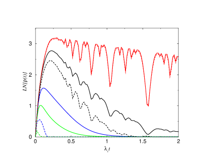
Figure 1: Logarithmic negativity as a function of time for different polariton self-interaction strengths and dissipation rates. See text for parameters.

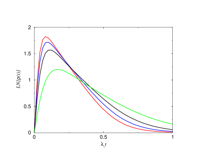
Figure 2: Logarithmic negativity as a function of time for different polariton populations. See text for parameters.

In Figure (1) we plot the time evolution of the polariton entanglement, $LN[\rho(t)]$, for a two trap cluster initially prepared with $|\alpha_{j}|^{2}=6$ (the amount of entanglement does not depend on the frequency $\omega_{j}$ of each trap). Four different values of dissipation rates $\Gamma=0.01,0.1,1$ and $3$ are considered and correspond in Fig.(1) to colors red, blue, black and green, respectively. Additionally, for each decay rate, results for two extreme values of the ratio between the intra-trap and inter-trap interactions are displayed: $\lambda_{j}/\lambda_{c}=1$ solid lines and $\lambda_{j}/\lambda_{c}=10$ dashed lines (colors are still as described above). The first observation is that entanglement is immediately generated by the polariton-polariton interaction, $\lambda_{c}$, and it is preserved for a significant fraction of the time that polariton population in the traps is maintained. The cluster system starts its evolution in a separable state rising its entanglement degree in an almost linear way with a slope depending directly on the initial polariton population, a clear indication of how important is the effective non-linear polariton interactions for generating entanglement. At long times the system ends again in a separable state, as it should be because the traps become empty and thus the final state is nothing but the double vacuum state. At very low decay rates entanglement oscillations are visible due to the quasi-unitary evolution of inter-trap correlations governed exclusively by $\lambda_{c}$ [8]. Note that in this limit of weak dissipation the entanglement dynamics does not depend on the intra-trap polariton interactions $\lambda_{j}$, as it is evident from the almost identical solid and dashed red curves in Fig.(1). As the dissipation becomes important populations and the entanglement decay faster. The polariton population follows a very simple exponential decay form given by $<\hat{a}^{{\dagger}}_{j}\hat{a}_{j}>(t)=|\alpha_{j}|^{2}e^{-2\Gamma t}$ while for the entanglement a more pronounced dependence on the polariton self-interactions are evident. Thus, dissipation and polariton self-interactions jointly degrade significantly both the maximum attainable entanglement and the time interval where entanglement is visible.

Figure (2) shows the time evolution of $LN(\rho)$ for different polariton initial populations $|\alpha_{j}|^{2}=10$ (red curve), $|\alpha_{j}|^{2}=8$ (blue curve), $|\alpha_{j}|^{2}=6$ (black curve) and $|\alpha_{j}|^{2}=3$ (green curve). Other parameters are: $\lambda_{1}=\lambda_{2}=-1$ and $\Gamma=1$. It is evident that the rising time of the entanglement is shorter as the polariton population increases, emphasizing previous comments on the importance of inter-trap polariton-polariton interactions for an efficient and rapid generation of entanglement. However, on the other hand, the temporal width of the entanglement curve decreases as a function of the polariton population, indicating the high level of non-linear effects occurring in the present system.

Some numerical estimates are in order. According to Ref.[2] typical engineered trap radius range from $5$ to $50$ $\mu m$. Pumping pulse lasers of low intensity on the order of $1$ $mW$ give rise to a polariton density of $10^{8}-10^{10}$$cm^{-2}$. Thus, for experimentally achievable trap sizes, typically $10-100$ polaritons could be found in a single small trap. Our unit of time is fixed by the inter-trap (or inter-species) interaction strength $\lambda_{c}$. According to Ref.[3], $\lambda_{c}\sim 10-100$ $\mu eV$, which for $\lambda_{c}t\sim 1$ yields to $t\sim 40$ $psec$. Hence, the theoretical results we discuss above are in the lower range of experimentally accessible polariton densities and time resolution, requiring very clean microcavities samples and high quality factors $Q$, for entanglement detection to be observable. However, our analytical results should be indeed valuable as a starting point for more numerically involved calculations in realistic situations.

4 Conclusions

By solving exactly the Master equation for an interacting trapped polariton system we have found that polariton entanglement can be immediately produced from an initial separable multi-coherent state. The entanglement starts rising linearly with a slope depending on the initial trap populations. The entanglement maximum is an increasing function of the initial number of polaritons. However, the entanglement duration time shortens as the initial trap population becomes large. In any case polariton entanglement observation would require very good microcavities with weak dissipation rates.

LQ acknowledges MEC(Spain) for a sabbatical grant and Universidad Autónoma de Madrid-Spain for hospitality during the development of the present work. This work has been supported in part by the Spanish MEC under contract QOIT Consolider-CSD2006-0019 and by CAM under contract S-0505/ESP-0200.

References

References

- [1] Balili R et al. 2007 Science 316 1007
- [2] Kim N Y et al. 2008 Phys.Stat.Sol. (b) 245 1076
- [3] Na N and Yamamoto Y 2008 Preprint quant-ph/0804.1829
- [4] Rodríguez F J, Quiroga L, Tejedor C, Martín M D, Viña L and André R 2008 Phys.Rev. B 78 035312
- [5] Ban M 1992 J.Math.Phys. 33 3213
- [6] Moya-Cessa H 2006 Phys.Reports 432 1
- [7] Vidal G and Werner R F 2002 Phys.Rev. A 65 032314
- [8] Quiroga L and Tejedor C to be published
- [9] Wootters W K 1998 Phys.Rev.Lett. 80 2245
- [10] Duan L-M, Giedke G, Cirac J I and Zoller P 2000 Phys.Rev.Lett. 84 2722
- [11] Simon R 2000 Phys.Rev.Lett. 84 2726