Exact potential-density pairs for flattened dark haloes

Abstract

Cosmological simulations suggest that dark matter haloes are not spherical, but typically moderately to strongly triaxial systems. We investigate methods to convert spherical potential-density pairs into axisymmetric ones, in which the basic characteristics of the density profile (such as the slope at small and large radii) are retained. We achieve this goal by replacing the spherical radius $r$ by an oblate radius $m$ in the expression of the gravitational potential $\Phi(r)$.

We extend and formalize the approach pioneered by Miyamoto & Nagai (1975) to be applicable to arbitrary potential-density pairs. Unfortunately, an asymptotic study demonstrates that, at large radii, such models always show a $R^{-3}$ disc superposed on a smooth roughly spherical density distribution. As a result, this recipe cannot be used to construct simple flattened potential-density pairs for dynamical systems such as dark matter haloes. Therefore we apply a modification of our original recipe that cures the problem of the discy behaviour. An asymptotic analysis now shows that the density distribution has the desired asymptotic behaviour at large radii (if the density falls less rapidly than $r^{-4}$). We also show that the flattening procedure does not alter the shape of the density distribution at small radii: while the inner density contours are flattened, the slope of the density profile is unaltered.

We apply this recipe to construct a set of flattened dark matter haloes based on the realistic spherical halo models by Dehnen & McLaughlin (2005). This example illustrates that the method works fine for modest flattening values, whereas stronger flattening values lead to peanut-shaped density distributions.

1 Introduction

The intrinsic shape of dark matter haloes in the Cold Dark Matter paradigm has been a matter of debate for the past two decades (e.g. Frenk et al., 1988; Dubinski & Carlberg, 1991; Warren et al., 1992; Cole & Lacey, 1996). The most recent numerical simulations of cosmological clustering in a $\Lambda$CDM framework suggest that dark matter haloes are typically slowly rotating, moderately to strongly triaxial systems, with an average flattening that increases with increasing halo mass (e.g. Jing & Suto, 2002; Hopkins, Bahcall & Bode, 2005; Bailin & Steinmetz, 2005; Kasun & Evrard, 2005; Allgood et al., 2006; Hayashi, Navarro & Springel, 2007). In order to set up realistic models for dark matter haloes, we need to leave the well-trodden path of spherical symmetry and consider structures that reflect this variety in shapes. A crucial step is the construction of exact flattened or triaxial potential-density pairs with a realistic density structure (for example a cuspy behaviour at small radii). The most straightforward way to construct such axisymmetric or triaxial potential-density pairs is to consider a spherical density profile $\rho(r)$ with the desired characteristics. If one replaces in this expression the spherical radius $r$ by an oblate spheroidal radius

$$m(R,z)=\sqrt{R^{2}+\frac{z^{2}}{q^{2}}},$$ (1)

or a triaxial radius

$$m(x,y,z)=\sqrt{x^{2}+\frac{y^{2}}{p^{2}}+\frac{z^{2}}{q^{2}}},$$ (2)

one obtains an axisymmetric or triaxial density profile $\rho_{\text{f}}({\boldsymbol{r}})\equiv\rho_{\text{f}}(m)$ whose isodensity surfaces are concentric oblate spheroids or ellipsoids with fixed axis ratios. This is a very straightforward recipe to construct simple oblate, prolate or triaxial density profiles, but unfortunately the formulae to calculate the corresponding potential $\Phi_{\text{f}}({\boldsymbol{r}})$ are cumbersome and can only be calculated numerically. In N-body or hydrodynamical simulations, the potential (or its gradient) has to be calculated very frequently and should be known with as efficiently and accurately as possible to avoid numerical artifacts. As a result, it is worthwhile to look for methods to create exact potential-density pairs for axisymmetric or triaxial configurations in which the potential can be calculated in a more straightforward way.

One general approach one can apply is to modify a spherical potential-density pair by adding a (finite) spherical harmonics expansion to it. While this approach can in principle be used to construct exact potential-density pairs for axisymmetric or triaxial systems (e.g. de Zeeuw & Carollo, 1996), the number of terms in the expansion typically has to be substantial, such that we approach a similar situation as before. An alternative approach to construct axisymmetric or triaxial potential-density pairs is to apply a transformation $r\rightarrow m$ on the potential rather than on the density. If we have an analytical expression for $\Phi_{\text{f}}({\boldsymbol{r}})\equiv\Phi_{\text{f}}(m)$, we can use Poisson’s equation to calculate the corresponding density distribution $\rho_{\text{f}}({\boldsymbol{r}})$. The advantage of this approach is that the calculation of the density $\rho_{\text{f}}({\boldsymbol{r}})$ from the potential $\Psi_{\text{f}}(m)$ requires only differentiations, such that one always obtains potential-density pairs in which both potential and density are analytical functions. One disadvantage is that one cannot a priori set the shape of the isodensity contours; it is not even guaranteed that the density corresponding to a given potential is everywhere positive. A second disadvantage is that simple recipes such as equation (1) do not work for the potential, because the isopotential surfaces need to become spherical at large radii. Other, unavoidably more complicated, recipes must be considered.

A successful example to construct an oblate analytical potential-density pair based on this strategy was the seminal work by Miyamoto & Nagai (1975). These authors create an exact potential-density pair by considering the spherical Plummer potential

$$\Phi(r)=-\frac{GM}{\sqrt{r^{2}+b^{2}}},$$ (3)

and turning it into a flattened potential

$$\Phi_{\text{f}}(R,z)=-\frac{GM}{\sqrt{R^{2}+\left(a+\sqrt{z^{2}+b^{2}}\right)^{2}}}.$$ (4)

The resulting density distribution can be calculated fairly easily. This technique of constructing flattened or triaxial potential-density pairs has been applied to other potentials by e.g. Satoh (1980), Zhenglu (2000) and Vogt & Letelier (2007). While this recipe provides a straightforward means to create analytical flattened potential-density pairs, it generates densities that do not correspond to astrophysical systems such as dark matter haloes. Indeed, at large radii the Miyamoto-Nagai type models show a notorious double behaviour, with a thin disc superposed on a roughly spherical density profile. While this could provide a first approximation for disc galaxies (although the density in galaxy discs is exponential rather than $R^{-3}$), this is obviously not the desired shape for a dark matter halo.

The goal of the present paper is to construct axisymmetric or triaxial potential-density pairs that can be used to model realistic dark matter haloes, starting from an arbitrary spherical potential-density pair. In Section 2 we formulate a recipe based on the Miyamoto & Nagai (1975) approach and we demonstrate that such models always have the conspicuous $R^{-3}$ disc-like behaviour at large radii, such that it cannot be used to represent dynamical systems as dark matter haloes. In Section 3 we adapt our recipe to cure this conspicuous behaviour and we demonstrate that this new recipe can produce analytical axisymmetric potential-density pairs which retain the original behaviour of the original density profile at both small and large radii. In Section 4 we apply this recipe to create a set of flattened potential-density suitable to represent dark matter haloes based on the spherical Dehnen & McLaughlin (2005) models. Section 5 sums up.

2 Miyamoto-Nagai type models

In order to create a set of oblate spheroidal models, we will replace the spherical radius $r$ in the spherical model by a spheroidal radius $m=m(R,z)$. We need to find a prescript such that $m$ is flattened at small radii and spherical at large radii. A general form that satisfies these requirements is

$$m\equiv m(R,z)=\sqrt{R^{2}+\frac{z^{2}}{Q^{2}(z)}},$$ (5)

where $Q(z)$ is a monotonically rising function of $z$ which has the asymptotic behaviour that it approaches 1 at large radii and a constant value $q$ at small radii. There are of course infinitely many different functions $Q(z)$ with these characteristics. Inspired by Miyamoto & Nagai (1975) we concentrate on one such particular function

$$Q(z)=\frac{z}{\sqrt{\left(a^{2}-b^{2}+\sqrt{z^{2}+b^{2}}\right)^{2}-a^{2}}},$$ (6)

for which we find

$$q=\sqrt{\frac{b}{a}}.$$ (7)

Substituting expression (6) into (5) we obtain

$$m(R,z)=\sqrt{R^{2}+\left(a-b+\sqrt{z^{2}+b^{2}}\right)^{2}-a^{2}}.$$ (8)

When we move to polar coordinates in the equatorial plane using $R=r\sin\theta$ and $z=r\cos\theta$, we find that at small radii

$$m(r,\theta)\sim\frac{\sqrt{\cos^{2}\theta+q^{2}\sin^{2}\theta}}{q}\,r,$$ (9)

whereas at large radii $m(r,\theta)\sim r$. The equipotential surfaces of the potential $\Phi_{\text{f}}(r,\theta)=\Phi_{\text{f}}(m)$ will hence be flattened with flattening $q$ at small radii and spherical at large radii, as required.

Once we have constructed the potential $\Phi_{\text{f}}(r,\theta)$, we can compute the corresponding density $\rho_{\text{f}}(r,\theta)$ that self-consistently generates this potential through Poisson’s equation.

$$\rho_{\text{f}}(r,\theta)=\frac{1}{4\pi r^{2}}\left[\frac{\partial}{\partial r}\left(r^{2}\,\frac{\partial m}{\partial r}\,\frac{{\text{d}}\Phi_{\text{f}}}{{\text{d}}m}\right)+\frac{1}{\sin^{2}\theta}\,\frac{\partial}{\partial\theta}\left(\sin\theta\,\frac{\partial m}{\partial\theta}\,\frac{{\text{d}}\Phi_{\text{f}}}{{\text{d}}m}\right)\right].$$ (10)

After some manipulation we can write this equation as

$$\rho_{\text{f}}(r,\theta)=T_{1}(r,\theta)\,\rho(m)+T_{2}(r,\theta)\,\bar{\rho}(m).$$ (11)

Here, $\rho(m)$ represents the density of the original spherical model evaluated at $r=m$ and $\bar{\rho}(m)$ is the average density of the original spherical model within a radius $r$,

$$\bar{\rho}(r)=\frac{M(r)}{\frac{4\pi}{3}r^{3}},$$ (12)

also evaluated at $r=m$. The coefficients $T_{1}$ and $T_{2}$ in equation (11) are independent of the potential of the system, and are given by

$$T_{1}(r,\theta)=\frac{r^{2}}{m^{2}}\left[\sin^{2}\theta+\left(1-\frac{G}{2F}\right)^{2}\frac{\cos^{2}\theta}{F^{2}}\right],$$ (13)

and

$$T_{2}(r,\theta)=\frac{r^{2}}{3m^{2}}\left[\left(\frac{1}{F}-1-\frac{2G}{F^{2}}-\frac{H}{2F^{2}}+\frac{G^{2}}{F^{3}}\right)\sin^{2}\theta+\left(2-\frac{2}{F}+\frac{G}{F^{2}}-\frac{H}{2F^{2}}+\frac{G^{2}}{4F^{3}}\right)\frac{\cos^{2}\theta}{F}\right],$$ (14)

with

$$F=Q^{2}(z),$$ (15)

$$G=z\,F^{\prime}(z),$$ (16)

$$H=z^{2}\,F^{\prime\prime}(z).$$ (17)

These coefficients are never divergent and it is straightforward to check that for the trivial case $a=b$, they reduce to $T_{1}\equiv 1$ and $T_{2}\equiv 0$, such that we recover the original spherical density distribution $\rho(r)$, as required.

The asymptotic expansion for the two coefficients $T_{1}$ and $T_{2}$ at large radii reads

$$T_{1}(r,\theta)\sim 1+\frac{(a-b)\,|\cos\theta|}{r},$$ (18)

$$T_{2}(r,\theta)\sim-\frac{a^{2}-b^{2}}{r^{2}}.$$ (19)

If the initial spherical model has a finite mass, the mean density $\bar{\rho}(m)$ behaves asymptotically as $r^{-3}$. If the density of the initial spherical model decreases more slowly than $r^{-5}$, the density of the corresponding oblate model will asymptotically reduce to the density of the spherical model.

There is one caveat, however: the asymptotic expansion for the coefficients $T_{1}$ and $T_{2}$ derived above is not valid within the equatorial plane $\theta=\tfrac{\pi}{2}$. Since $z=0$ in the entire equatorial plane, we have by construction $F=q^{2}$ and $G=H=0$ at every position $R=r=m$ in the equatorial plane, such that we have the identities

$$T_{1}\left(R,\tfrac{\pi}{2}\right)\equiv 1,$$ (20)

$$T_{2}\left(R,\tfrac{\pi}{2}\right)\equiv\frac{1-q^{2}}{3q^{2}}=\frac{a-b}{3b}.$$ (21)

In the equatorial plane, the contribution of the second term in (11) will not decrease as $R^{-5}$, but only as $R^{-3}$, and it will therefore dominate the contribution of the first term. The mean density term $\bar{\rho}(m)$ is only dominant at large radii in the equatorial plane, such that the final density $\rho_{\text{f}}(r,\theta)$ will have a discy structure at large radii, with a thin $R^{-3}$ disc superposed on a nearly spherical density profile. This behaviour is present in all Miyamoto-Nagai type models (Miyamoto & Nagai, 1975; Satoh, 1980; Zhenglu, 2000) and unfortunately turns this recipe unsuitable for the construction of realistic flattened dark matter halo models.

3 A new recipe to construct flattened models

3.1 Construction

An inconvenience about the family of models presented in the previous section was the appearance of a discy structure at large radii. At large radii, the density profiles of the models behave similarly as their spherical progenitors, at all polar angles except in the equatorial plane $z=0$. Mathematically, the reason for this discy structure is the discontinuous asymptotic behaviour of the function $Q(z)$. Outside the equatorial plane, $|z|\rightarrow\infty$ and $Q\rightarrow 1$ at large radii, such that the coefficient $T_{2}$ disappears. In the equatorial plane, however, $z$ is always equal to zero and $T_{2}$ does not converge to zero, such that the mean density term $\bar{\rho}(m)$ contributes to (and dominates) the density.

If we want to construct a set of models which do not show this discy structure at large radii, we can try to adapt the recipe from the previous section in a way that $Q$ smoothly goes to one at large radii, both inside and outside the equatorial plane. This can be achieved by replacing the oblate radius $m$ from equation (5) by

$$m(R,z)=\sqrt{R^{2}+\frac{z^{2}}{Q^{2}(r)}}.$$ (22)

Using the functional form (6) for $Q(r)$, we obtain

$$m(R,z)=\sqrt{R^{2}+\frac{z^{2}}{r^{2}}\left[\left(a-b+\sqrt{r^{2}+b^{2}}\right)^{2}-a^{2}\right]}.$$ (23)

or

$$m(r,\theta)=\sqrt{r^{2}\sin^{2}\theta+\cos^{2}\theta\left[\left(a-b+\sqrt{r^{2}+b^{2}}\right)^{2}-a^{2}\right]}.$$ (24)

This new oblate radius $m$ has a similar asymptotic behaviour at small and large radii as the original version (8). Replacing $r$ by this oblate radius $m$ in the expression $\Phi(r)$ for the potential of a spherical model, we obtain an oblate axisymmetric potential $\Phi_{\text{f}}(r,\theta)$. The density that self-consistently generates this potential can be found through Poisson’s equation. Going through a similar analysis as in the previous Section, we find that the density can be written as

$$\rho_{\text{f}}(r,\theta)=U_{1}(r,\theta)\,\rho(m)+U_{2}(r,\theta)\,\bar{\rho}(m),$$ (25)

where the coefficients $U_{1}$ and $U_{2}$ are now given by

$$U_{1}(r,\theta)=\frac{r^{2}}{m^{2}}\left[\sin^{2}\theta+\frac{1-G}{F^{2}}\,\cos^{2}\theta+\frac{G}{F^{2}}\left(1-\frac{1}{F}+\frac{G}{4F^{2}}\right)\cos^{4}\theta\right],$$ (26)

and

$$U_{2}(r,\theta)=\frac{r^{2}}{3m^{2}}\left[\left(\frac{1}{F}-1\right)+\left(1+\frac{1}{F}-\frac{2}{F^{2}}-\frac{H}{2F^{2}}+\frac{G^{2}}{F^{3}}\right)\cos^{2}\theta+\frac{1}{F^{2}}\left(\frac{H}{2}-\frac{G^{2}}{F}-\frac{H}{2F}+\frac{G^{2}}{4F^{2}}\right)\cos^{4}\theta\right],$$ (27)

with now obviously

$$F=Q^{2}(r),$$ (28)

$$G=r\,F^{\prime}(r),$$ (29)

$$H=r^{2}\,F^{\prime\prime}(r).$$ (30)

Again, it is elementary to check that for $U_{1}\equiv 1$ and $U_{2}\equiv 0$ for the trivial case $a=b$.

3.2 The asymptotic behaviour at large radii

After some algebra, one obtains that the asymptotic expansion of the coefficients $U_{1}$ and $U_{2}$ at large radii becomes

$$U_{1}(r,\theta)\sim 1,$$ (31)

$$U_{2}(r,\theta)\sim-\frac{2\,(a-b)\cos 2\theta}{3r}.$$ (32)

These expansions are valid for all directions; in particular, there is no different behaviour of these components in the equatorial plane. Comparing the asymptotic behaviour of these coefficients to those of the previous Section, we see that the coefficients $T_{1}$ and $U_{1}$ both have an asymptotic behaviour with simply 1 as the leading term, such that the first term in the total density (11) or (25) behaves identically as the density of the original spherical model. The coefficients $T_{2}$ and $U_{2}$ behave in a different way, however: while $T_{2}$ decreases as $r^{-2}$ at large radii, $U_{2}$ decreases only as $r^{-1}$, with an additional $\cos 2\theta$ azimuthal dependence. Only for those models where the density of the initial spherical model decreases more slowly than $r^{-4}$, the density of the corresponding flattened model will asymptotically reduce to the density of the spherical model. For models where the density decreases more rapidly at large radii, the density will be dominated by the second term. As this term becomes negative at large radii near the rotation axis, such models are unacceptable. This method to flatten spherical potential-density pairs is therefore limited to those models where the density decreases more slowly than $r^{-4}$. This is typically the case for dark matter haloes.

3.3 The asymptotic behaviour at small radii

The goal of this paper was to consider a method to, starting from a spherical potential-density pair, construct a flattened analog that preserves the asymptotic behaviour of the density profile at both small and large radii. An asymptotic analysis of the functions $U_{1}$ and $U_{2}$ learns that both terms converge to a finite value at small radii,

$$U_{1}(r,\theta)\sim\frac{1}{q^{2}}\,\frac{\cos^{2}\theta+q^{4}\sin^{2}\theta}{\cos^{2}\theta+q^{2}\sin^{2}\theta},$$ (33)

$$U_{2}(r,\theta)\sim\frac{1-q^{2}}{3q^{2}}\,\frac{q^{2}\sin^{2}\theta-2\cos^{2}\theta}{\cos^{2}\theta+q^{2}\sin^{2}\theta}.$$ (34)

Assume that our density profile $\rho(r)$ behaves as a power law at small radii,

$$\rho(r)\sim\rho_{0}r^{-\gamma_{0}},$$ (35)

with $0\leqslant\gamma_{0}<3$. It is easy to check that the mean density $\bar{\rho}(r)$ has a similar slope,

$$\bar{\rho}(r)\sim\frac{3\rho_{0}}{3-\gamma_{0}}\,r^{-\gamma_{0}}.$$ (36)

Combining the expressions (9), (25), (33), (34), (35) and (36), we find the asymptotic behaviour of $\rho_{\text{f}}(r,\theta)$ at small radii,

$$\rho_{\text{f}}(r,\theta)\sim\frac{\rho_{0}}{3-\gamma_{0}}\frac{(1-\gamma_{0}q^{2}+2q^{2})\,q^{2}\sin^{2}\theta+(1-\gamma_{0}+2q^{2})\cos^{2}\theta}{q^{2-\gamma_{0}}\,(\cos^{2}\theta+q^{2}\sin^{2}\theta)^{1+\gamma_{0}/2}}\,r^{-\gamma_{0}},$$ (37)

This result demonstrates that the asymptotic behaviour of the original spherical model is preserved after the flattening: the slope of the density profile remains, only the zero point changes and becomes dependent of the polar angle $\theta$. In particular, along the major and minor axes we find the expansions

$$\rho_{\text{f}}(R,\tfrac{\pi}{2})\sim\rho_{0}\,\frac{1-\gamma_{0}q^{2}+2q^{2}}{(3-\gamma_{0})\,q^{2}}\,R^{-\gamma_{0}},$$ (38)

$$\rho_{\text{f}}(z,0)\sim\rho_{0}\,\frac{1-\gamma_{0}+2q^{2}}{(3-\gamma_{0})\,q^{2-\gamma_{0}}}\,z^{-\gamma_{0}},$$ (39)

Using these expressions, we easily find the expression for the flattening $q_{\rho}$ of the isodensity surfaces at small radii,

$$q_{\rho}\sim\left(\frac{1-\gamma_{0}+2q^{2}}{1-\gamma_{0}q^{2}+2q^{2}}\right)^{1/\gamma_{0}}q.$$ (40)

For modest flattening ($q\lesssim 1$) we find a nearly linear relation,

$$1-q_{\rho}\sim\left(\frac{5-\gamma_{0}}{3-\gamma_{0}}\right)(1-q).$$ (41)

Apart from the well-known fact that the isodensity surfaces are generally more flattened than the isopotential surfaces, this equation illustrates that the flattening of the inner isodensity surfaces increases with increasing $\gamma_{0}$.

4 Application: flattened Dehnen-McLaughlin dark halo models

As an application of the formalism we have described in the previous section, we construct in this section a set of flattened dark matter halo models. Our starting point is the general three-parameter family of generalized NFW models or Zhao models

$$\rho(r)=\rho_{0}\,\left(\frac{r}{r_{0}}\right)^{-\gamma_{0}}\left[1+\left(\frac{r}{r_{0}}\right)^{\eta}\right]^{-(\gamma_{\infty}-\gamma_{0})/\eta}.$$ (42)

The density of this general model is characterized by a power law with (negative) slopes $\gamma_{0}$ and $\gamma_{\infty}$ at respectively small and large radii. The third parameter, $\delta$, is a measure of the width of the transition region between the two power-law zones. This three-parameter model, the general dynamical properties of which are described by Saha (1993) and Zhao (1996), includes a large variety of well-known simple potential density pairs used extensively throughout the literature to describe dynamical systems ranging from galactic nuclei to dark matter haloes (e.g. Plummer, 1911; Jaffe, 1983; Hernquist, 1990; Dehnen, 1993; Tremaine et al., 1994; Navarro, Frenk, & White, 1997).

To demonstrate our recipe to construct oblate dark matter haloes, we focus on a particular, non-trivial subset of this general three-parameter set of models presented by Dehnen & McLaughlin (2005). These authors used the Jeans equations to derived the density profile of a self-gravitating spherically symmetric dynamical system that satisfy two characteristics of dark haloes observed in cosmological simulations. The first of these characteristics is the mysterious power-law behaviour of the so-called pseudo phase-space density $Q=\rho/\sigma^{3}$ with $\sigma(r)$ the velocity dispersion (Taylor & Navarro, 2001; Ascasibar et al., 2004; Rasia, Tormen, & Moscardini, 2004). The second ingredient in their model is a linear relation between the logarithmic density slope and the anisotropy, observed in different haloes with radically different formation histories (Hansen & Moore, 2006; Hansen & Stadel, 2006). Constrained by these two assumptions, together with the assumption of spherical symmetry, Dehnen & McLaughlin (2005) derived a dark matter halo density of the form (42), with

$$\gamma_{0}=\frac{7+10\beta_{0}}{9},$$ (43)

$$\gamma_{\infty}=\frac{31-20\beta_{0}}{9},$$ (44)

$$\eta=\frac{4-2\beta_{0}}{9},$$ (45)

$$\rho_{0}=\frac{10-5\beta_{0}}{18\pi}\,\frac{M}{r_{0}^{3}}$$ (46)

with $\beta_{0}$ the value of the velocity anisotropy parameter at small radii and $M$ the total mass. The gravitational potential that generates this mass density is

$$\Phi(r)=-\frac{9}{4-2\beta_{0}}\,\frac{GM}{r_{0}}\,B_{\frac{1}{1+(r/r_{0})^{\eta}}}\left(\frac{9}{4-2\beta_{0}},\frac{11-10\beta_{0}}{4-2\beta_{0}}\right),$$ (47)

with $B_{x}(p,q)$ the incomplete Beta function.

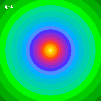
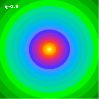
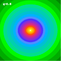
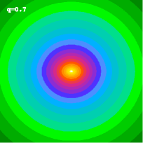
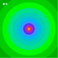
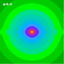
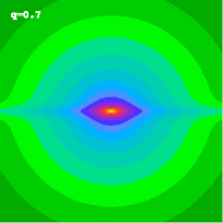
Figure 1: Isopotential (top row) and isodensity (bottom row) plots in the meriodional plane of the Dehnen & McLaughlin (2005) halo models flattened according to the Miyamoto-Nagai type flattening from Section 2. Different models are shown according to different values of the potential flattening parameter $q$, ranging from 1 to 0.7. Each plot has dimensions of $10a\times 10a$. At large radii, the isodensity surfaces are discy with an $R^{-3}$ dependence in the equatorial plane.

We constructed flattened versions of the spherical Dehnen & McLaughlin (2005) haloes with $\beta_{0}=0$ and $r_{0}=a$ using the recipes of Sections 2 and 3. In Figure 1 we plot the isopotential and isodensity surfaces in the meridional plane for the Miyamoto-Nagai type models for different values of the parameter $q=b/a$. The isopotential surfaces (top row) are nearly spheroidal, and the flattening decreases smoothly from the centre (where the axis ratio is equal to $q$) to spherical at large radii. The bottom row shows the isodensity surface plots of the corresponding models. The isodensity surfaces are nearly spheroidal in the central regions with a flattening that is much stronger than the flattening of the potential. For increasing radii, the isodensity surfaces become increasingly lemon-shaped, and at large radii, they become very discy with an $R^{-3}$ dependence in the equatorial plane, in agreement with the results from Section 2. Obviously, these models can not represent realistic dark haloes.

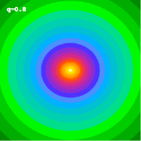
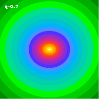
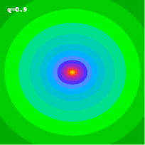
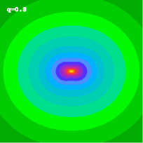
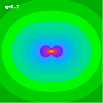
Figure 2: Similar to Figure 1, but now the models are flattened according to the adapted recipe from Section 3. The shape of the isopotential surfaces is slightly smoother near the equatorial plane, which causes the discy structure at large radii in the isodensity surfaces to disappear. Instead, the isodensity surfaces remain roughly spheroidal with a flattening that smoothly disappears for increasing radii.

In Figure 2 we plot in a similar way the isopotential and isodensity surfaces for flattened haloes according to the recipe of Section 3. Compared to Figure 2, the shape of the isopotential surfaces is hardly different, with just a small alteration (a smoother behaviour) near the equatorial plane. This minor change does affect the large-scale behaviour of the isodensity surfaces significantly: the discy structure at large radii disappears and the isodensity surfaces remain roughly spheroidal with a flattening that smoothly disappears for increasing radii.

For models with a modest potential flattening ($0.9\lesssim q\leqslant 1$), all isodensity surfaces are nearly spheroidal, with a flattening parameter $q_{\rho}$ ranging from roughly 0.8 at the centre to 1 at large radii. For stronger flattening parameters, the shape of the isodensity surfaces at small radii becomes increasingly more peanut-shaped, as progressively more mass has be located near the equatorial plane (and progressively less mass near the symmetry axis) in order to stretch the isopotential surfaces into an oblate shape. This net transfer of mass from the symmetry axis to the equatorial plane cannot continue for ever. At a certain stage, a negative density will arise around on either side of the equatorial plane, causing physically unacceptable models.

5 Discussion and conclusion

In this paper, we have investigated methods to convert spherical potential-density pairs into axisymmetric ones, in which the basic characteristics of the density profile (such as the slope at small and large radii) are retained. We attempted this by replacing the spherical radius $r$ by an oblate radius $m$ in the expression of the gravitational potential $\Phi(r)$. The advantage of this approach is that the calculation of the corresponding density via Poisson’s equation requires only differentiations, such that one always obtains fully analytical potential-density pairs. Disadvantages are that one cannot a priori set the shape of the isodensity surfaces and that the standard recipe for the oblate radius $m$ cannot be used since the isopotential surfaces need to become spherical at large radii.

In Section 2 we have considered a recipe inspired by the flattening of the Plummer potential-density pair by Miyamoto & Nagai (1975). We have extended and formalized this mechanism to be applicable to arbitrary potential-density pairs. The recipe is sufficiently simple: the density can formally be written as a simple linear combination of the original spherical density $\rho(m)$ and the mean density $\bar{\rho}(m)$ –both evaluated at the oblate radius $m$– and the coefficients are simple, non-divergent functions independent of the potential-density pair. Unfortunately, an asymptotic study demonstrates that, at large radii, such models always show a $R^{-3}$ disc superposed on a smooth roughly spherical density distribution. As a result, this recipe cannot be used to construct simple flattened potential-density pairs for dynamical systems such as early-type galaxies or dark matter haloes.

In Section 3 we have applied a modification of our original recipe that cures the problem of the discy behaviour. The new models can be constructed in a similar manner as the Miyamoto-Nagai type models from Section 2; only the coefficients in the linear combination of $\rho(m)$ and $\bar{\rho}(m)$ are different. An asymptotic analysis now shows that the density distribution has the desired asymptotic behaviour at large radii (if the density falls less rapidly than $r^{-4}$). We also show that the flattening procedure does not alter the shape of the density distribution at small radii: while the inner density surfaces are flattened, the slope of the density profile is unaltered. We have applied this recipe to construct a set of flattened dark matter haloes based on the realistic spherical halo models by Dehnen & McLaughlin (2005). This example illustrates that the method works fine for modest flattening values ($0.9\lesssim q\leqslant 1$ with $q$ the flattening of the isopotential surfaces at small radii), whereas stronger flattening values lead to peanut-shaped density distributions.

For the sake of simplicity, we have focused this work on the construction of flattened potential-density pairs, but there is no reason why the recipe applied here should be limited to an oblate geometry. The procedure is readily applicable to prolate or triaxial geometries, which seems necessary to represent the general population of dark matter haloes.

References

- Ascasibar et al. (2004) Ascasibar Y., Yepes G., Gottlöber S., Müller V., 2004, MNRAS, 352, 1109
- Allgood et al. (2006) Allgood B., Flores R. A., Primack J. R., Kravtsov A. V., Wechsler R. H., Faltenbacher A., Bullock J. S., 2006, MNRAS, 367, 1781
- Bailin & Steinmetz (2005) Bailin J., Steinmetz M., 2005, ApJ, 627, 647
- Cole & Lacey (1996) Cole S., Lacey C., 1996, MNRAS, 281, 716
- Dehnen (1993) Dehnen W., 1993, MNRAS, 265, 250
- Dehnen & McLaughlin (2005) Dehnen W., McLaughlin D. E., 2005, MNRAS, 363, 1057
- de Zeeuw & Carollo (1996) de Zeeuw P. T., Carollo C. M., 1996, MNRAS, 281, 1333
- Dubinski & Carlberg (1991) Dubinski J., Carlberg R. G., 1991, ApJ, 378, 496
- Frenk et al. (1988) Frenk C. S., White S. D. M., Davis M., Efstathiou G., 1988, ApJ, 327, 507
- Hansen & Moore (2006) Hansen S. H., Moore B., 2006, NewA, 11, 333
- Hansen & Stadel (2006) Hansen S. H., Stadel J., 2006, JCAP, 5, 14
- Hayashi, Navarro & Springel (2007) Hayashi E., Navarro J. F., Springel V., 2007, MNRAS, 377, 50
- Hernquist (1990) Hernquist L., 1990, ApJ, 356, 359
- Hopkins, Bahcall & Bode (2005) Hopkins P. F., Bahcall N. A., Bode P., 2005, ApJ, 618, 1
- Hubble (1926) Hubble E. P., 1926, ApJ, 64, 321
- Jaffe (1983) Jaffe W., 1983, MNRAS, 202, 995
- Jing & Suto (2002) Jing Y. P., Suto Y., 2002, ApJ, 574, 538
- Kasun & Evrard (2005) Kasun S. F., Evrard A. E., 2005, ApJ, 629, 781
- Miyamoto & Nagai (1975) Miyamoto M., Nagai R., 1975, PASJ, 27, 533
- Navarro, Frenk, & White (1997) Navarro J. F., Frenk C. S., White S. D. M., 1997, ApJ, 490, 493
- Plummer (1911) Plummer H. C., 1911, MNRAS, 71, 460
- Rasia, Tormen, & Moscardini (2004) Rasia E., Tormen G., Moscardini L., 2004, MNRAS, 351, 237
- Saha (1993) Saha P., 1993, MNRAS, 262, 1062
- Satoh (1980) Satoh C., 1980, PASJ, 32, 41
- Taylor & Navarro (2001) Taylor J. E., Navarro J. F., 2001, ApJ, 563, 483
- Toomre (1963) Toomre A., 1963, ApJ, 138, 385
- Tremaine et al. (1994) Tremaine S., Richstone D. O., Byun Y.-I., Dressler A., Faber S. M., Grillmair C., Kormendy J., Lauer T. R., 1994, AJ, 107, 634
- Vogt & Letelier (2007) Vogt D., Letelier P. S., 2007, PASJ, 59, 319
- Warren et al. (1992) Warren M. S., Quinn P. J., Salmon J. K., Zurek W. H., 1992, ApJ, 399, 405
- Zhao (1996) Zhao H., 1996, MNRAS, 278, 488
- Zhenglu (2000) Zhenglu J., 2000, MNRAS, 319, 1067