INTEGRAL and XMM-Newton spectroscopy of GX 339–4 during Hard/Soft Intermediate and High/Soft States in the 2007 outburst

Abstract

We present simultaneous XMM-Newton and INTEGRAL observations of the luminous black hole transient and relativistic jet source GX 339–4. GX 339–4 started an outburst on November of 2006 and our observations were undertaken from January to March of 2007. We triggered five INTEGRAL and three XMM-Newton target of Opportunity observations within this period. Our data cover different spectral states, namely Hard Intermediate, Soft Intermediate and High/Soft. We performed spectral analysis to the data with both phenomenological and more physical models and find that a non-thermal component seems to be required by the data in all the observations. We find a hardening of the spectrum in the third observation coincident with appearance of a broad and skewed ${\rm Fe}$ ${\rm K}_{\alpha}$ line. In all spectral states joint XMM/EPIC-pn,JEM-X, ISGRI and SPI data were fit with the hybrid thermal/non-thermal Comptonization model (EQPAIR). While this model accounts very well for the high/energy emission observed, it has several drawbacks in the description of the lower energy channels. Our results imply evolution in the coronal properties, the most important one being the transition from a compact corona in the first observation to the disappearance of coronal material in the second and re-appearance in the third. This fact, accompanied by the plasma ejection events detected in radio on February 4 to 18, suggest that the ejected medium is the coronal material responsible for the hard X-ray emission.

1 Introduction

GX 339–4 (also called V821 Ara) is a recurrent black hole transient X-ray binary (i.e. this source undergoes frequent outbursts followed by very faint states) with few episodes in quiescence (e.g. Kong et al. (2000)). Hynes et al. (2003) determined, on the basis of optical spectroscopic observations, that this source has an orbital period of 1.7 days and a mass function of $f(M)=5.8{\pm}0.5\,M_{\odot}$ (since $f(M){\propto}M\sin^{3}(i)$, note that this represents a lower limit to the black hole mass). The distance and the spectral type of the secondary star are uncertain. Hynes et al. (2004) established the distance to be 6-15 kpc depending on the spectral type of the secondary (a subgiant), being later than F spectral type. Therefore, this black hole transient is a low-mass X-ray binary (LMXB). Slightly later, on the basis of binary parameters determination, Zdziarski et al. (2004) suggested the distance to be ${\gtrsim}7$ kpc, consistent with Hynes et al. (2004). The inclination of this binary system is known to be low, from the small emission-line velocity amplitudes observed. Wu et al. (2001) determined a plausible value for the inclination of $i=15^{\circ}$ from spectroscopic data. Miller et al. (2004a), Miller et al. (2004b) and Miller (2006a) found that fits of the relativistic Fe $K_{\alpha}$ line imply a very low value of the inclination ($i=20-30^{\circ}$) as well. The latter corresponds to the inner disk inclination, i.e. not the inclination of the binary plane.

The timing and spectral properties of GX 339–4 required a re-interpretation of the standard classification scheme of the black hole states. The behavior of GX 339–4 supports the view that, as reviewed by Homan et al. (2001) and van der Klis (2006), X-ray states are important, but are not a simple function of the luminosity. As claimed by Homan et al. (2005), another variable apart from the mass accretion rate, $\dot{M}$, drives black hole state transitions and at least two factors must drive state transitions; the second factor may be, e.g., the compactness of the corona (Homan et al. (2001)). Black hole X-ray transients and related states (Tanaka et al. (1995); Chen et al. (1997); McClintock & Remillard (2006)) provide an excellent opportunity to investigate the importance of irradiation and non-thermal processes in the X-${\gamma}$-ray spectra of X-ray binaries. Black hole binary outbursts typically begin and end in the low/hard state, with a high-energy spectrum that can be roughly described by a powerlaw with a spectral index ${\Gamma}$ varying in the range 1.4-2.1. At some point in the outburst (coinciding with the presence of radio outflows) the source transits from the hard intermediate (HIMS) to soft intermediate (SIMS) states, characterized by a quenching of the radio emission (i.e. the so-called jet line). Then, the thermal disk component luminosity increases and the high energy powerlaw is softer (${\Gamma}=1.5-2.5$) (Miyamoto et al. (1991a), Belloni et al. (1997), Homan & Belloni (2005), see van der Klis (2006) for a review). The transition between these states occurs very rapidly; they were found in EXOSAT observations of GX 339–4 by Mendez & van der Klis (1997). The Very/High (hereafter VH) state was first observed in GX 339–4 (Miyamoto et al., 1991a), when very peculiar X-ray variability was detected with Ginga/LAC (6 Hz QPO, 10-60 s duration dips and ”flip-flops”). Miyamoto et al. (1991b) even proposed a jet model in order to account for the observed time variability in this state, on the basis of the size of the Comptonizing coronae inferred from observations of GX 339–4 in the VH state (Miyamoto et al., 1991a). Recent studies (Homan et al. (2001), Mendez & van der Klis (1997), Klein-Wolt & van der Klis (2007)) point out that the VH state is really an intermediate state but at a different luminosity level.

Since its diskovery more than 30 years ago by Markert et al. (1973), the source has been extensively studied with several optical, infrared, X-ray and ${\gamma}$-ray observatories. At higher energy its emission has been studied by all the major observatories, i.e., GRANAT/SIGMA (Grebenev et al. (1993), Bouchet et al. (1993)), CGRO/OSSE (Grabelsky et al., 1995), CGRO/BATSE (Harmon et al. (1994), Rubin et al. (1998)), ASCA (Wilms et al. (1999)), Ginga (Ebisawa et al. (1993) and Ueda et al. (1994)), RXTE (e.g. Zdziarski et al. (2004), Belloni et al. (1999)) and INTEGRAL (Joinet et al. (2007), Belloni et al. (2006)). Homan et al. (2005) presented a multi-wavelength study of the 2002 outburst and suggested a non-thermal jet origin for the optical/near-infrared emission in the low/hard state, while the accretion disk dominates in the high/soft state. This source is very intriguing in the optical, since its photometric optical behavior shows a very low amplitude modulation superposed by some flickering events. In addition to the QPOs detected in X-rays (usually appearing in the low/hard state and maintained in the intermediate states, while quenched in the high/soft state; see e.g. Belloni et al. (2005)), this source also shows optical QPOs (${\rm f}{\approx}0.064$ Hz; Motch et al. (1982), Steiman-Cameron et al. (1997)). A very interesting issue is also the occurrence of optical states corresponding to the X-ray states (Motch et al. (1983), Motch et al. (1985)). This kind of variability is difficult to explain if optical radiation comes from reprocessing of X-rays and seems to demands optical activity originated in the base of a jet.

GX 339–4 may harbor a black hole with a high spin parameter. Miller et al. (2004a) and Reis et al. (2008) found very small inner disk radius of $2-3\,{\rm R_{g}}$ (where $R_{g}=GM/c^{2}$ and $a=cJ/GM^{2}$; see Bardeen et al. (1972) and Thorne (1974)), implying a dimensionless spin parameter of $a>0.8-0.9$ (Miller, 2006a). Relativistic radio jets with $v/c>0.9$ have recently been observed, detected (Gallo et al., 2004) during a transition from the low/hard to the high/soft state, therefore increasing the list of known microquasars showing similar radio and X-ray properties. A radio jet is usually reported in the low/hard state of GX 339–4, for which Fender et al. (1999) reported a quenching of the radio emission during the high/soft state (by a factor of ${\geq}25$ compared to the low/hard state). The low/hard state would be associated by a steady state of the outflow (Corbel et al. (2000), Fender (2001), Gallo et al. (2003)). It was also proposed that during state transitions the radio emission results in one or more discrete ejection events, as already observed by Gallo et al. (2004) during their detection of jets. GX 339–4 shares X-ray timing and spectral properties with the classical black hole Cyg X-1, although the former exhibits more frequent state changes and a larger dynamic range of soft X-ray luminosity (Tanaka et al. (1995),Zdziarski et al. (1998), Nowak et al. (1999)).

While the physical nature of the soft component is commonly associated with an optically thick accretion disk, there is no consensus about the origin of the hard powerlaw component, where a powerlaw is probably a simplification of a much more complex reality. The energy spectra include also additional components, important for the physics of accretion, such as the Fe $K_{\alpha}$ fluorescence feature (see, e.g., Miller (2007), Reynolds & Nowak (2003)) and Compton reflection bump, both being different aspects of the same physical origin (i.e. fluorescence of the Fe ions and Compton back-scattering, respectively, both being the most obvious reactions of an irradiated disk by a high-energy source; George & Fabian (1991)). An extremely high ionisation may inhibit the formation of emission and absorption lines in the inner disk, which would explain the lack of Fe $K_{\alpha}$ fluorescence emission line in some systems. One important parameter to measure is the presence/absence of a high energy cut-off in the spectrum, for which observations at energies $>20$ keV are necessary. It is known since a long time (Sunyaev & Titarchuk (1980),Grove et al. (1998)) that the spectrum in the low/hard state show a cut-off around $100$ keV. This cut-off was interpreted as being a consequence of the thermal (inverse) Comptonization of photons from the disk on a distribution of electrons thought to represent a corona (for which the geometry is a matter of debate).

In this paper we report on spectral analysis of simultaneous INTEGRAL and XMM/EPIC-pn data, during five and three Target of Opportunity observations of GX 339–4, respectively, occurring between 2007 January 30 and March 31 (epochs 1–5 below; see Table 1 for more details). We fit the obtained spectra with phenomenological models in Section 3.1 and we observed that the source spectral states evolved from one observation to the other, as reported in Section 3.2. Fits of the spectrum with both phenomenological and Comptonization models are presented in Section 3.1, 5 and 4 and we end with the discussion of the results in Section 6.

2 Observations

In 2006 November, X-ray activity of GX 339–4 was detected with the Rossi X-ray Timing Explorer (RXTE; Swank et al. (2006)). The source had an almost constant flux until end of December 2006, when the hard (15-50 keV) X-ray flux increased by a large amount. It reached its brightest level since 2004 November, as detected by SWIFT/BAT (Krimm et al., 2006). At the end of January 2007, observations were triggered with the INTEGRAL satellite (Miller et al., 2007). During the following months, the source underwent an evolution from the low/hard to softer states, as shown in preliminary results reported in Caballero-Garcia et al. 2007a-e. Observations in radio with ATCA during February 4 to 18 revealed that the source was undergoing a series of plasma ejection events (Corbel et al., 2007). Our INTEGRAL observations cover 5 Target of Opportunity observations of ${\approx}130$ ks each, spread from 2007 January 30 to March 31 (see Table 1). We also carried out a series of 3 ToO observations with the XMM-Newton satellite, simultaneous with the second, third and fifth INTEGRAL observations. Details about the dates and exposure times appear in Table 1.

2.1 INTEGRAL

The data described were obtained with INTEGRAL, using the following instruments: the SPectrometer on INTEGRAL (SPI; Vedrenne et al. (2003)), the INTEGRAL IBIS Soft Gamma-Ray Imager (ISGRI; Lebrun et al. (2003)) and the Joint European X-ray Monitor (JEM-X; Lund et al. (2003). SPI, ISGRI and JEM-X allow images to be obtained through the coded mask technique. ISGRI is optimized for 15 keV to 1 MeV imaging and SPI is optimized for high-resolution spectroscopy in the 18 keV to 8 MeV band. The former provides an angular resolution of $12^{\prime}$ full-width half maximum (FWHM) and an energy resolution, $E/{\Delta}E$ of ${\approx}12$ (FWHM) at 100 keV. SPI provides an angular resolution of $2.8^{\circ}$ (FWHM) and an $E/{\Delta}E$ of $430$ FWHM at 1.3 MeV. JEM-X has a fully coded Field of View (FOV) of $4.8^{\circ}$ diameter and an angular resolution of $3^{\prime}$ FWHM, with a spectral resolution of 1.2 keV (FWHM) at 10 keV. JEM-X has a spectral resolution of $E/{\Delta}E=0.2$ at 6 keV, thus providing medium resolution spectral capabilities in the energy range of 3–35 keV.

The difference in the (effective) exposure times between the INTEGRAL instruments given in Table 1 (JEM-X, ISGRI and SPI) are due to the difference in the dead times and variation in the efficiency along the fields of view. The dithering pattern used during the observations was $5{\times}5$ (square of 25 pointings separated by 2.17 degrees centered on the main target of the observation); this is the best pattern in order to minimize background effects for the SPI and ISGRI instruments in crowded fields. Data reduction was performed using the standard Off-line Science Analysis (OSA) 7.0 software package available from the INTEGRAL Science Data Centre (ISDC).

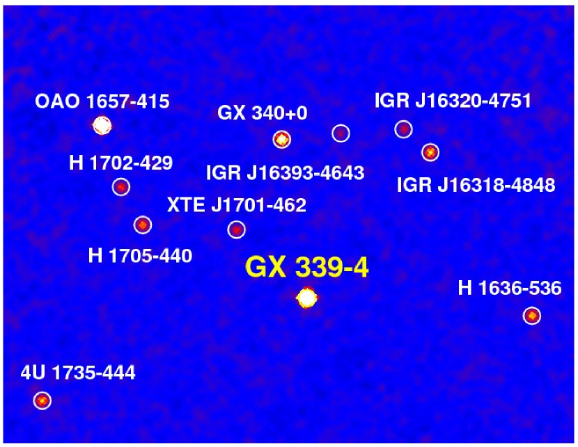
Figure 1: Mosaic significance image (obtained in epoch 1) of the GX 339–4 region as seen with ISGRI in the $20-40$ keV energy range, galactic coordinates from right to left. Besides GX 339–4 (detection isgnificance of $1\,070{\sigma}$), several other high energy sources are visible.

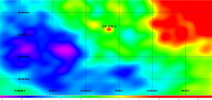
Figure 2: Significance map obtained with SPIROS in the 200–300 keV energy range during epoch 1 observations; the color scale goes from -5 ${\sigma}$ to 5 ${\sigma}$; the grid spacing is of 1 ^∘ and 5 ^∘ in right-ascension and declination, respectively. GX 339–4 is the only source detected in the 200–300 keV energy range, with a flux of $0.01951{\pm}0.004030$ ph/cm${}^{2}/$sec (4.8 ${\sigma}$).

Because of the steep fall in response off-axis in the case of JEM-X, and because of its reduced FOV (${\approx}5^{\circ}$ of diameter), we limited the pointing radius with respect to the GX 339–4 position to be within $4^{\circ}$. In the case of SPI and ISGRI, with large Fully Coded Fields of Views (FCFOV) ($16^{\circ}{\times}16^{\circ}$ for SPI and $9^{\circ}{\times}9^{\circ}$ for ISGRI), pointing selections were not necessary. In total, 149, 254 and 107 pointings (or Science Window – each having exposure times lasting from 1800 to 3600 s) data were used for SPI, ISGRI and JEM-X, respectively. The difference in the number of pointings between SPI and ISGRI is due to the fact that in epoch 4 and 5 the source was too weak in hard X-rays ($E>20$ keV) to be detected with SPI. Due to the fact that SPI is a high resolution spectrograph in its energy range (20-8 000 keV), it is not optimized for the detection of sources without taking into account previous information about the spatial distribution of them. Thus, we used the list of found sources obtained with ISGRI in the (20-40) keV mosaic images (see Figure 1) as our input catalog. This resulted in GX 339–4 as the only source detected in the 200–300 keV energy range (Figure 2) with a detection significance of 4.8${\sigma}$.

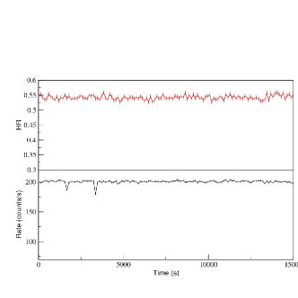
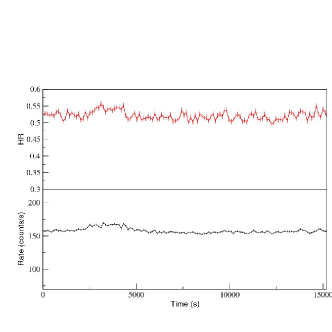
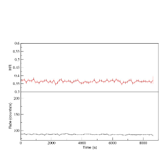
Figure 3: Lower panels: 0.6-10 keV EPIC pn light curve of GX 339–4 for epochs 2 (upper-left panel), 3 (upper-right panel) and 5 (bottom panel).Upper panels: hardness ratio (counts in the 2–10 keV band divided by those between 0.6–2 keV) for epochs 2, 3 and 5. The binning is 120 s for all panels.

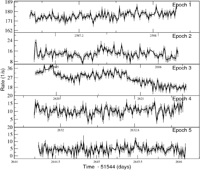
Figure 4: ISGRI/INTEGRAL (20-200 keV) light curve during all the observations (from Epoch 1 to 5). The binning is 1 000 s for all panels.

We combined single revolution SPI spectra from epochs 1–3, considering that there was no significant evolution within each revolution (as shown by the relative constancy of the INTEGRAL and XMM-Newton light curves, except for epoch 3 –see below–; Figures 3 and 4), in order to increase the signal to noise ratio. We obtained 3 SPI spectra in total. The same was done for the low energy instruments (JEM-X and ISGRI), thus obtaining five spectra, namely one for each epoch (see Table 1). We applied 2$\%$ systematic errors to the JEM-X, ISGRI and SPI spectra. We restricted our analysis in the energy ranges of $5-20$, $18-200$ and $23-300$ keV for the JEM-X, ISGRI and SPI spectral analysis, as recommended. The SPI and ISGRI spectra were rebinned at high energies (${\gtrsim}200$ keV) with the FTOOL grppha procedure to reach the detection level of $2{\sigma}$ per spectral bin.

2.2 XMM/EPIC-pn

The XMM-Newton Observatory (Jansen et al., 2001) includes three 1 500 cm² X-ray telescopes each with an European Photon Imaging Camera (EPIC; 0.1–15 keV) at the focus. Two of the EPIC imaging spectrometers use MOS CCDs (Turner et al., 2001) and one uses pn CCDs (Strüder et al., 2001). The Reflection Grating Spectrometer; (RGS; 0.35–2.5 keV, Den Herder et al., 2001) are located behind two of the telescopes. In addition, there is a co-aligned 30 cm diameter Optical/UV Monitor telescope (OM, Mason et al., 2001), providing simultaneous coverage with the X-ray instruments.

GX 339–4 was observed by XMM-Newton for 16.8 ks on 2007 February 19 (hereafter called Obs 1 and coinciding with INTEGRAL Epoch 2), for 17.8 ks on 2007 March 5 (hereafter called Obs 2 and coinciding with INTEGRAL Epoch 3) and for 20 ks on 2007 March 30 (hereafter called Obs 3 and coinciding with INTEGRAL Epoch 5). We refer to Table 1 for details.

The thin optical blocking filter was used with the EPIC camera. The EPIC pn camera was operated in burst mode due to the high count rate of the source (from $\gtrsim$6700 s^-1 to $\gtrsim$3000 s^-1 for Obs 1 to 3, respectively). For the same reason, the EPIC MOS cameras were not operated. The individual RGS1 and RGS2 CCD chips were read out sequentially. This reduces the frame time from 4.8 to 0.6 seconds (4.8/8) and consequently the pile-up by almost an order of magnitude. All the X-ray data products were obtained from the XMM-Newton public archive and reduced using the Science Analysis Software (SAS) version 7.1.0. In pn burst mode, only one CCD chip (corresponding to a field of view of 13$\farcm$6$\times$4$\farcm$4) is used and the data from that chip are collapsed into a one-dimensional row (4$\farcm$4) to be read out at high speed, the second dimension being replaced by timing information. The duty cycle is only 3$\%$. This allows a time resolution of 7 $\mu$s, and photon pile-up occurs only for count rates above 60 000 s^-1. Only single and double events (patterns 0 to 4) were selected. Ancillary response files were generated using the SAS task arfgen. Response matrices were generated using the SAS task rmfgen. In this paper we do not use RGS spectra because our main aim is to make a study of the continuum properties of the spectra.

PN Charge Transfer Inneficiency (CTI) rate dependency has been observed for count rates $>200-300$ cts/s, i.e. for very bright sources CTI correction overpredicts the CTI losses. This can result in an up to 2$\%$ apparent gain shift most visible for spectral features like edges or lines . Hereafter, we applied $2\%$ systematic errors to the EPIC-pn spectra reported below. We used EPIC ${\rm pn}$ data in the 0.7–10 keV energy range.

2.3 Light curves

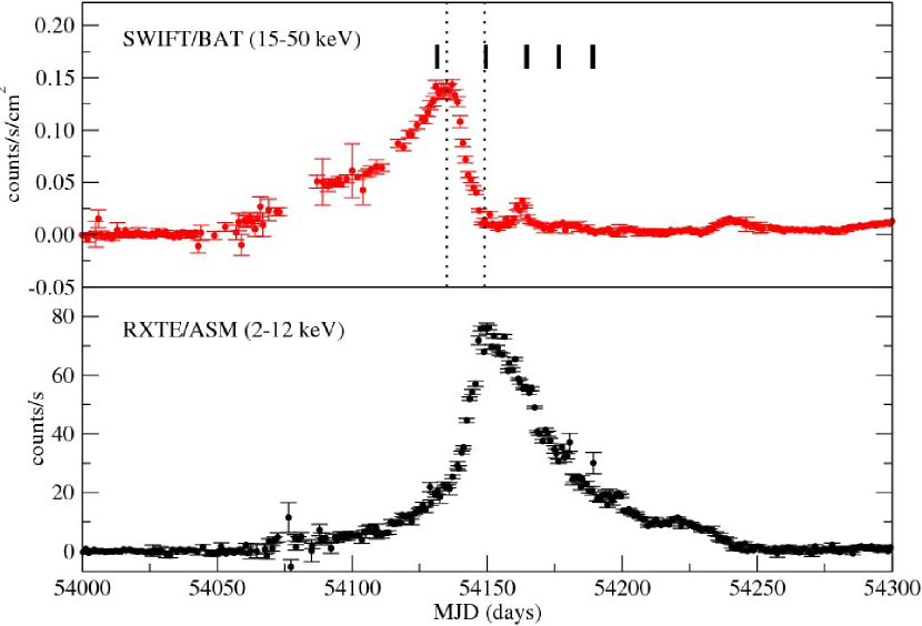
Figure 5: SWIFT/BAT and RXTE/ASM daily light curves of GX 339–4 during the overall outburst in 2007 (red and black dotted lines, respectively), illustrating the spectral evolution between the different states. Intervals of time in which the INTEGRAL observations were undertaken (solid black lines) and the period of time when the radio ejection events were detected (within both dotted black vertical lines) are also shown.

In Figure 5, we show the SWIFT/BAT and the RXTE/ASM light curve in the 15–50 keV and 2–12 keV energy ranges during the entire outburst. The horizontal lines shown in the Figure indicate the time intervals (150 ks each, in five observations) over which our average spectra were obtained. Note that black hole transients usually begin and end their outbursts in the low/hard state (see Nowak (1995); Fender et al. (2004); Homan & Belloni (2005)), and the 2007 outburst of GX 339–4 is no exception. As can be seen in Figure 5, the beginning of the outburst started earlier at high energies (15–50 keV) rather than in softer X-rays (2–12 keV), when observations of epoch 1 were made. The other four epochs were made during a period when the source spectrum was much softer. It is interesting to notice the sudden increase of $15\%$ flux (with respect to the maximum value) of the 15–50 keV light curve, during the transition from second to third epoch observations, possibly associated with changes in the high-energy emission source, as we will discuss in Section 6.

In Figure 3 we show the XMM/EPIC-pn light curves in the 0.6–10 keV energy range and calculated hardness ratio (counts in 2–10 keV band divided by counts in 0.6–2 keV) with a time binning of 120 s. We do not see spectral evolution during the time of each observation due to the constancy of both the light curves and hardness ratio (except for a small increase in the flux during a short time period in epoch 3, but of the order of ${\leq}6$%).

In Figure 4 we show the ISGRI (20–200 keV) light curves during all the observations. The source was significantly detected during all the epochs with decreasing flux (except for epoch 3, with higher flux than for epoch 2). Within every epoch the flux was relatively constant, except for epoch 3, in which the flux was decreasing with time, with a total flux variation of 70% around the mean flux value. In spite of this, we combined all the revolution data to get the spectrum in this epoch as well (as did for the remainder epochs) in order to get higher signal to noise ratio.

3 Analysis of spectra

We performed fits to the combined JEM-X, ISGRI and, when available, SPI and XMM/EPIC-pn spectra, for each of the five epochs (see Table 1) using XSPEC (Arnaud, 1996) v.11.3. All errors quoted in this work are 90% confidence errors, obtained by allowing all variable parameters to float during the error scan. The hydrogen column density was set to be free when XMM/EPIC-pn data were available and fixed at ${\rm N}_{\rm H}=0.5{\times}10^{22}$ ${\rm atom}$ cm^-2 (Dickey & Lockman, 1990) when only INTEGRAL data were available.

Our main aim in these fits is to characterize the broad continuum thanks to the broad XMM-Newton and INTEGRAL spectral coverage. To account for uncertainties in relative instrument calibrations, we fixed JEM-X multiplicative calibration constant to 1 and let that of ISGRI and SPI free to vary in the fits for the different data sets as shown in Table 2. In the case of using both INTEGRAL and XMM/EPIC-pn spectra, we fixed the EPIC-pn multiplicative constant to 1 and let that of JEM-X, ISGRI and SPI free to vary, in order to account for cross-calibration uncertainties as well . The presence of an XMM/EPIC-pn instrumental line was clear in the spectra of epochs 2 and 3 and we added a gaussian emission line centered at $2.28$ keV and $2.25{\pm}{0.03}$ keV, respectively. For epoch 5 two absorption instrumental lines appeared, centered at $1.82$ keV and $2.14$ keV, respectively. As mentioned in the XMM-Newton analysis of GRO J1655–40 (Díaz Trigo et al., 2007); where these features were present as well, structured residuals near 2.3 keV are probably due to an incorrect instrumental modeling of the Au mirror edges, whilst those near 1.8 keV are probably due to an incorrect modeling of the Si absorption in the CCD detectors.

3.1 Fits of joint XMM/EPIC-pn and INTEGRAL spectra with phenomenological models

We performed preliminary fits to the spectra of every single epoch with the phenomenological model consisting of a multicolor disk black body (diskbb in XSPEC) of Mitsuda et al. (1984) plus a powerlaw convolved by absorption at low energy in order to describe the high-energy emission. In none of the observations this model provided a good fit to the data (${\chi}^{2}_{\nu}=46,3.05,4.2,1.8,3.3$ for ${\nu}=96,150,154,46,108$ for epochs 1, 2, 3, 4 and 5, respectively).

In epoch 1 the situation improved dramatically (${\chi}^{2}_{\nu}=2.76$, ${\nu}=94$) when a high-energy cut-off was included in the model (i.e. constant*phabs(diskbb + powerlaw)highecut; ${\rm E}_{\rm c}{\approx}70$ keV). Nevertheless, some positive and negative residuals still remained at 6–10 keV and 10–20 keV, in the form of a steepening of the spectrum and of an edge, respectively, indicating the likely presence of a broad ${\rm Fe}$ ${\rm K}_{\alpha}$ line. We included a broad ${\rm Fe}$ gaussian line centered at ${\rm E}_{\rm Fe}=6.4-6.97$ keV, getting the final statistics of ${\chi}^{2}_{\nu}=1.4$ (${\nu}=91$). With the model constant*phabs(diskbb+gaussian+powerlaw)highecut, the final values obtained for the photon index and the folding energy are of ${\Gamma}=1.46^{+0.03}_{-0.02}$ and $E=66.4^{+0.9}_{-1.1}$ keV, respectively. These values resemble those found by Belloni et al. (2006) during the HIMS of the 2004 outburst.

In epoch 2 low-energy positive residuals in the form of an excess near 1 keV were detected in the XMM/EPIC-pn spectrum and the fit greatly improved when considered (${\chi}^{2}_{\nu}=1.9$, ${\nu}=144$). The obtained equivalent width is $W_{1\,keV}=11.6{\pm}2.1$ eV. This feature is detected in a number of X-ray binaries and has been previously modeled either as an emission line, or as an edge, and its nature is unclear (e.g. Kuulkers et al. (1997); Sidoli et al. (2001); Boirin et al. (2003), Díaz Trigo et al. (2007)). However, since this has not been detected before in GX 339–4 we think that this line probably is an instrumental effect due to incorrect modeling of ${\rm Ne}$ ${\rm IX}$ and ${\rm Ne}$ ${\rm X}$ and ${\rm Fe}$ ${\rm L}$ in the CCD detector.

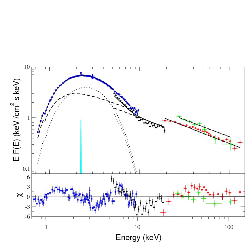
Figure 6: The plot above shows the residuals obtained when the INTEGRAL and XMM-Newton data of epoch 3 is fit with a phenomenological disk plus power-law model. In the residuals a relativistically broadened ${\rm Fe}$ ${\rm K}_{\alpha}$ line is present.

In epoch 3 positive and negative residuals appeared, centered at ${\approx}6-10$ keV and ${\approx}10-20$ keV, respectively (see Figure 6). These residuals are compatible with a broad and skewed ${\rm Fe}$ ${\rm K}_{\alpha}$ line and the respective ${\rm Fe}$ edge. As in epoch 1, we added a gaussian line centered at ${\rm E}_{\rm Fe}=6.4-6.97$ keV and the fit improved (${\chi}^{2}_{\nu}=3.3$, ${\nu}=146$), but some residuals in the red wing of the ${\rm Fe}$ line (3–5 keV) still remained. These residuals point out to the ${\rm Fe}$ ${\rm K}_{\alpha}$ line having a relativistic origin (i.e. originated very close to the black hole). Thus, we substituted the gaussian component by a laor (Laor, 1991) model, which includes general relativity effects in the modeling of the X-ray emission in the inner boundaries of a rotating black hole. The parameters of this model are the line energy $E$, the disk emissivity index $q$ (where the emissivity is assumed to have a power-law form of $J(r){\propto}r^{-q}$; where $q=3$ is expected for a standard disk), the inner radius of the line emission region in units of $GM/c^{2}$ (with a lower limit of 1.235 $R_{g}$ for a maximally rotating black hole), the outer line emission radius in units of $GM/c^{2}$ (fixed to the fiducial value of 100 $R_{g}$), the disk inclination, and the line normalization. With this model, we obtained significant better statistics (${\chi}^{2}_{\nu}=2.7$, ${\nu}=143$) and flat residuals in the 3–5 keV energy range, where the relativistic effects of the ${\rm Fe}$ complex are expected to appear . The inner radius of the disk, the emissivity index, the disk inclination and the normalization were free to vary in the fit. We allowed the value of the inclination to vary in the range 10^∘–60^∘. The value obtained for the line energy is very high ($6.83{\pm}0.14$ keV), indicating a very ionized medium. The obtained value for the emissivity index is rather steep ($q=5.2^{+0.5}_{-1.0}$), being close to the value found in the VH state ($q=4.8-6$ by Miller et al. (2004a)). The obtained value for the disk inclination is $i=35^{+4}_{-7}$^∘. High values for the emissivity index indicate that the primary source is very close to the black hole. Steep emissivity indices (${\approx}7$) have been observed from a number of Seyfert galaxies (e.g. Fabian et al. (2004); Fabian et al. (2005)). The inner radius obtained was rather low ($r_{in}=2.11{\pm}0.11$ $R_{g}$), thus being clearly different from 6 $R_{g}$ (expected value for a non-rotating Schwarzschild black hole) and close to the value found by Reis et al. (2008) ($r_{in}=2-2.1$ $R_{g}$). The presence of negative residuals at 10 keV led us to consider the effects of a smoothed absorption of the $Fe$ ions in the inner disk. We included a smoothed absorption edge (smedge in XSPEC) and the fit improved, getting the final statistics of ${\chi}^{2}_{\nu}=1.3$ (${\nu}=141$). Relativistic smearing is expected to appear in the inner parts of the accreting disk and, with $Fe$ line, accounts phenomenologically for reflection. This resulted in an edge energy of $E_{\rm smedge}=8.53{\pm}0.20$ keV, compatible with He-like configuration for $Fe$ and ${\tau}=1.09^{+0.15}_{-0.11}$, with a smeared edge width frozen to $W_{\rm smedge}=5$ keV (close to the value found by Reis et al. (2008) in the VH state; i.e. $W_{\rm smedge}=4.5^{+0.5}_{-2.0}$ keV).

In epoch 4 some residuals remained in the form of a smeared edge in the 10–20 keV energy range. When considered (i.e. model constant*smedge*phabs(diskbb + powerlaw)), the fit improved (${\chi}^{2}_{\nu}=1.2$, ${\nu}=44$), meaning an F-test probability of 1.337E-04 that the improvement was made by chance. The value obtained for the threshold energy and the maximum absorption factor at threshold are $E_{\rm smedge}=9.53^{+0.5}_{-0.6}$ keV and ${\tau}=1.6{\pm}0.5$, respectively, compatible with H-like configuration for $Fe$.

Finally, in epoch 5, residuals in the form of an excess at ${\gtrsim}50$ keV and a smeared edge at 7–10 keV (${\chi}^{2}_{\nu}=3.3$, ${\nu}=108$) were present. In the residuals there was an emission line like in epoch 2 and we included an emission gaussian line centered at ${\approx}1$ keV (${\chi}^{2}_{\nu}=2.4$, ${\nu}=105$). The equivalent width obtained was $W_{1\,keV}=29{\pm}5$ eV, thus higher than in epoch 2. When adding the smoothed edge (i.e. model constant*smedge*phabs(diskbb + powerlaw + gaussian)) the fit greatly improved (${\chi}^{2}_{\nu}=1.3$, ${\nu}=104$). The obtained values for both the threshold energy and maximum absorption factor at threshold are $E_{\rm smedge}=9.22{\pm}0.25$ keV and ${\tau}=3.0{\pm}0.5$, respectively, the former compatible with H-like configuration for $Fe$ . The value for the absorption factor at threshold is very high and would indicate that it is not due to the presence of an absorber, rather being due to reflection effects. The excess above 50 keV would indicate an important source of Comptonization by non-thermal particles, as occurring in epoch 1, as shown below.

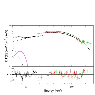
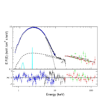
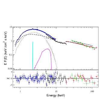
Figure 7: Unfolded INTEGRAL and XMM/EPIC-pn spectra (blue, black, red and green for the XMM/EPIC-pn, JEM-X, ISGRI and SPI data, respectively) from epochs 1 to 3 (upper-left to lower-right) fit with descriptive phenomenological models. The continuum line shows the total model (see the text Section 3.1 and Table 2 for details), the dotted and dashed lines show the accretion disk and the powerlaw components, respectively, and the magenta line represents relativistically broadened ${\rm Fe}$${\rm K}_{\alpha}$ emission from a disk. The cyan colored gaussian lines mean instrumental XMM/EPIC-pn effects.

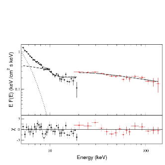
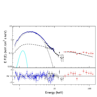
Figure 8: For epochs 4 and 5 spectral evolution occurred in the form of a gradual softening. See Section 3.1 for more details.

The values obtained for the best fit parameters with the best phenomenological fit are shown in Table 2 and the spectra with the best fit results are shown in Figures 7 and 8. In Table 3 we summarize the values for the photon indices of the powerlaw (analyzed in this Section) and un-absorbed luminosities of both the powerlaw and the disk (assuming a distance to the source of 8.5 kpc).

3.2 State classification and related behavior

The main features of the spectrum of epoch 1 are a rather flat photon index (${\Gamma}=1.46^{+0.03}_{-0.02}$) and the clear presence of a high-energy cut-off at $66.4^{+0.9}_{-1.1}$ keV. The value found for the cut-off is very close to the value reported by Belloni et al. (2006) ($E_{c}=70^{+10}_{-8}$ keV) during HIMS, although the value found for the photon index in their case was clearly steeper (${\Gamma}=1.92{\pm}0.05$). We conclude that the spectrum of epoch 1 corresponds in luminosity (Belloni et al. (1997), Fender et al. (2004), Homan & Belloni (2005)) and spectral characteristics to the HIMS. During epochs 2 and 3 the spectra are characterized by a steep high-energy emission (${\Gamma}{\approx}2.33{\pm}0.02,2.659^{+0.004}_{-0.01}$ for epochs 2 and 3, respectively). In the classification scheme of Homan & Belloni (2005), both correspond to the SIMS. The value of the photon index from epoch 2 resembles those reported previously by Nespoli et al. (2003) (${\Gamma}=2.44{\pm}0.10$) and Belloni et al. (2006) (${\Gamma}=2.3$) during SIMS of GX 339–4 as well. The inner disk temperatures found are $0.891{\pm}0.003$ keV and $0.852^{0.005}_{-0.008}$ keV, thus resembling the values found by Malzac et al. (2006) and Cadolle Bel et al. (2005) (i.e. $1.2{\pm}0.2$ keV) for Cyg X–1 in Intermediate states as well. Observations of GX 339–4 during the 2004 outburst by Miller et al. (2004a) during the VH state show the same photon index value for the high-energy emission (i.e. ${\Gamma}=2.61^{+0.09}_{-0.01}$) as us for epoch 3, accompanied by a detection of a relativistic $Fe$ line, as well. Indeed, in the most recent state prescription (Homan & Belloni, 2005), the VH state is the same as the SIMS.

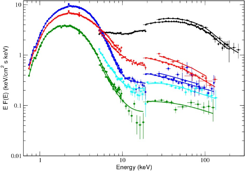
Figure 9: Unfolded spectra from epoch 1 to 5 (black, blue, red, cyan and green, respectively).

The spectrum during epochs 4 and 5 is characterized by a steep high-energy emission (${\Gamma}=2.39{\pm}0.06,2.65{\pm}0.02$). As can be seen in Figure 3 the hardness ratio (defined as HR=(2-10) keV)/(0.2-2) keV) of the light curves are very soft in epochs 4 and 5. The inner disk temperatures found for these epochs are $0.75^{+0.07}_{-0.06}$ keV and $0.698{\pm}0.003$ keV, respectively, thus resembling the values found in the HS state for Cyg X-1 (i.e. 0.6 keV Gierliński et al. (1999), Frontera et al. (2001)). The softness, the inner disk temperatures, the values for the photon index and the high value for the disk normalization component suggest that the source in those epochs is in the high/soft state, considering the classification scheme of Homan & Belloni (2005). The spectral evolution is presented in Figure 9.

As explained above, our observations of GX 339–4 cover the spectral evolution from the HIMS to high/soft state, passing through the SIMS. As shown in Section 3.1 and in Table 3, this spectral evolution involves very significant spectral changes which are strongly correlated. The changes in the spectral shape are strongly correlated with the ratio of the powerlaw to the disk luminosity. In the first epoch there was almost no disk contribution in the spectrum. It showed a cut-off at ${\rm E}_{\rm c}=66.4^{+0.9}_{-1.1}$ keV in the powerlaw. The cut-off disappeared in the second epoch and the powerlaw emission decreased notably, being just $1/7$ of the disk luminosity. In the third epoch the spectrum hardened again considerably (the powerlaw luminosity being 1.7 times higher than the disk luminosity, the latter decreased by $50\%$ with respect to the second epoch). The total luminosity increased by 50% in the transition from epoch 1 to 2 and remained more or less unchanged during epochs 2 and 3, while decreasing in epoch 4 and 5 (again decreased by $50\%$). The luminosities obtained for all the epochs were within the range of $20-50\%$ the Eddington luminosity (assuming the compact object being a black hole of $6{\rm M}_{\odot}$).

4 The high-energy excess

During the LH state of the GX 339–4 outburst occurring in 1991, a high-energy excess (above 200 keV) was observed with OSSE (Johnson et al. (1993), Wardziński et al. (2002)). In 2004, during the increasing phase of the 2004 outburst, Joinet et al. (2007) observed a similar feature with SPI when GX 339–4 was in its canonical LH state. Similar features have been recently reported for other black hole transients in LH states observed during the decreasing phase of their outbursts (Kalemci et al. (2006), Kalemci et al. (2005)). It is also more commonly associated with state transitions (Malzac et al., 2006) and with soft states (Gierliński et al., 1999).

Such a hard tail is ussually attributed to the presence of a small fraction of non-thermal electrons in the hot Comptonizing plasma. In the HIMS of our observations (epoch 1), GX 339–4 shows a highly significant cut-off at $66.4^{+0.9}_{-1.1}$ keV. This indicates that soft photons are Comptonized by a thermal electron population with a temperature $kT_{e}$ that is related to the cut-off energy. Both for the HIMS (epoch 1) and SIMS (epochs 2 and 3) non-negligible values of ${\ell}_{nth}/{\ell}_{h}$ were found (as shown below in Section 5).

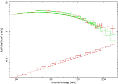
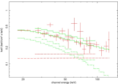
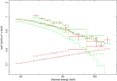
Figure 10: IBIS and SPI unfolded energy spectra for epochs 1, 2 and 3 (left to right) fit with a Comptonization model (COMPPS) plus a powerlaw.

In order to investigate further the possible presence of a non-thermal component during the HIMS and SIMS, IBIS and SPI spectra have been fit with the COMPPS model of Poutanen & Svensson (1996) (see Table 4). In this thermal Compton model, the spectrum is computed for a homogeneus spherical hot corona, inside which blackbody photons are injected and then upscattered by hot Maxwellian electrons. The reflected spectrum is smeared out by rotation of the disk due to special and general relativistic effects using diskline-type kernel. As in the comptt model (Titarchuk, 1994), the corona is parametrized by its electron temperature, $T_{e}$, and the radial Thompson optical depth, ${\tau}=n_{e}{\sigma}_{T}H$, where $n_{e}$ is the electron density, ${\sigma}_{T}$ is the Thompson cross section and $H$ the radius of the sphere. Using this thermal Comptonization model, some residuals are present at high-energy, especially in the spectrum of epoch 1. In order to mimic the presence of a non/thermal component, we added a powerlaw to the pure Comptonization model (see Figure 10). This led to an improvement of the ${\chi}^{2}$ that is significant for epoch 1 (see Table 4). The F-test probability that this improvement was made by chance is $p=6.461E-02$ for epoch 1. On the contrary, because of the low statistics in epochs 2 and 3, adding a powerlaw to the thermal Comptonization model is not required. However, we notice that the electron temperatures obtained with the thermal Compton plus powerlaw model are rather close to the values obtained with EQPAIR fits for all the epochs.

5 Fits of joint XMM/EPIC-pn and INTEGRAL spectra with the hybrid thermal/non-thermal Comptonization EQPAIR model

5.1 The model

We saw in the previous Section that a high-energy excess is visible in the spectra. Since this high-energy excess can not be well described by thermal Comptonization, we go into more sophisticated models containing a hybrid distribution of thermal/non-thermal particles. From the variety of Comptonization models available in the literature, we have chosen the hybrid thermal/non-thermal Comptonization EQPAIR model (Coppi, 2000), and relativistic line emission and disk reflection. The best-fit values for the parameters for all the epochs are shown in Table 5. Because the presence of an instrumental line at ${\approx}1$ keV in the XMM/EPIC-pn spectra of epochs 2, 3 and 5 was analyzed in Section 3.1, this will not be discussed further.

In the EQPAIR model, emission of the disk/corona system is modeled by a spherical hot plasma cloud with continuous acceleration of electrons illuminated by soft photons from the accretion disk. At high-energies the distribution of electrons is non-thermal, but at low energies a Maxwellian distribution with temperature $kT_{e}$ is established.

The disk spectrum incident in the plasma is modeled as coming from a pseudo-Newtonian accretion disk (${\tt diskpn}$ in XSPEC) extending from $R_{out}=100$ $R_{g}$ down to the minimum stable orbit $R_{out}=6$ $R_{g}$. Its spectral shape is then characterized by the maximum color temperature of the disk, $kT_{pn}$. Previous observations of Cyg X-1 with X-ray telescopes indicate temperatures ranging from 0.1 keV in the LH state up to 0.6 keV in the HS state (Gierliński et al. (1999), Frontera et al. (2001)).

The model (EQPAIR) takes into account angle dependence, Compton scattering (up to multiple orders), photon pair production, pair annihilation, bremsstrahlung, as well as reflection from a cold disk. This model includes ionized Compton reflection (as the pexriv model in XPSEC; Magdziarz & Zdziarski (1995)). The reflection component is smeared out by rotation of the disk due to special and general relativistic effects using diskline-type kernel to relativistic motion in the disk (as in the diskline model in XSPEC; Fabian et al. (1989)). We used the LAOR model (Laor, 1991) to model the relativistic iron line emission, with the emissivity index (${\beta}$) free and tied to the opposite value of that of the EQPAIR. The disk reflection component is calculated for neutral material with standard abundances, unless otherwise noted. We asumed free inclination and inner disk radius in the range of $10^{\circ}-60^{\circ}$ and $2-6$ $R_{g}$. The outer disk radius was fixed to 100 $R_{g}$.

The EQPAIR model provides the injection of a non-thermal electron distribution with Lorentz factors between ${\Gamma}_{min}$ and ${\Gamma}_{max}$ and a powerlaw spectral index ${\Gamma}_{inj}$. The system is characterized by the power (i.e. luminosity) $L_{i}$ supplied by its different components. We express each of them dimensionlessly as a compactness parameter, ${\ell}_{i}=L_{i}{\sigma}_{\rm T}/(Rm_{e}c^{3})$, where $R$ is the characteristic dimension and ${\sigma}_{\rm T}$ the Thompson cross-section of the plasma. Thus, ${\ell}_{s}$, ${\ell}_{th}$, ${\ell}_{nth}$ and ${\ell}_{h}={\ell}_{th}+{\ell}_{nth}$ correspond to the power in a soft disk entering the plasma, thermal electron heating, electron acceleration and the total power supplied to the plasma. The total number of electrons (not including ${\rm e}^{+}{\rm e}^{-}$ pairs) is determined by ${\tau}_{\rm T}$, the corresponding Thompson optical depth, measured from the center to the surface of the scattering region. If we consider injection from pairs ${\rm e}^{+}{\rm e}^{-}$, then the total optical depth of the thermalized scattering electrons/pairs is expected to be ${\tau}_{\rm T}{\geq}{\tau}_{\rm P}$.

In general, the spectral shape is insensitive to the exact value of the compactness, but it depens strongly on the compactness ratios (${\ell}_{h}/{\ell}_{s}$ and ${\ell}_{nth}/{\ell}_{h}$). Thus, we froze ${\ell}_{s}$ to a fiducial value (${\ell}_{s}=10$), as commonly reported for other sources with similar characteristics (e.g. Ibragimov et al. (2005)). In the fits reported below, we fit the data with a powerlaw distributed injection of electrons and compare with the results obtained with a mono-energetic distributed injection of them as well. The former distribution is expected in the case of shock acceleration of particles, while the second could be achieved in reconnection events that are expected to power the corona (Galeev et al., 1979).

5.2 Fits to the data

For the first epoch of our observations, due to the low disk contribution, we froze the disk temperature to a fiducial value of $kT_{pn}=300$ eV, as an intermediate value between LH and HS values found by Gierliński et al. (1999) and Frontera et al. (2001) for Cyg X–1. The relativistic Fe disk line emission was significant (with a chance probability of 4.823E-05). The most relevant factor is the inclination angle of the reflecting material, clearly favouring high values. We obtained worse residuals and statistics (${\chi}^{2}_{\nu}=1.8$, ${\nu}=82$) for the case of $i=30^{\circ}$ with respect to the case of $i=50^{\circ}$ (${\chi}^{2}_{\nu}=1.0$, ${\nu}=82$). Since this value is in conflict with the value obtained in Section 3.1 and the values obtained from fitting the X-ray data in the literature, we will adopt $i=30^{\circ}$ in the fits of the remainder epochs . High values for the ionization are preferred by the data, with an improvement of ${\Delta}{\chi}_{\nu}^{2}=0.5$ (for 82 d.o.f) with respect to the neutral case. The spectral cut-off already noticed in Section 3.1 can be modeled here by Comptonization of thermal distributed particles and reflection from a cold disk. As shown in Petrucci et al. (2001), with an electron temperature of $kT_{e}=27.5{\pm}1.2$ keV and an optical depth of ${\tau}=2.39^{+0.15}_{-0.18}$, it is possible to reproduce the spectral cut-off at $66.4^{+0.9}_{-1.1}$ keV. The spatial distribution of the Comptonizing particles is compact (${\ell}_{h}/{\ell}_{s}=3.9^{+0.6}_{-0.3}$) and mildly non-thermal (${\ell}_{nth}/{\ell}_{h}=0.40^{+0.15}_{-0.03}$). The high-energy distribution is well fit with a powerlaw injection of non-thermal electrons with relatively low photon index (${\Gamma}_{inj}=1.80^{+0.07}_{-0.05}$) with Lorentz factors within the range 1.3–100 (as considered in the remainder epochs as well). This issue means the clear presence of non-thermal particles in the plasma. When fitting with a mono-energetic distribution of electrons with a Lorentz factor of ${\Gamma}=5$, the fit slightly worsened (${\chi}^{2}_{\nu}=1.1$, ${\nu}=83$ and worse description of the highest energy emission) with respect to the previous fit (i.e. ${\chi}^{2}_{\nu}=1.0$, ${\nu}=82$). Albeit not significant, the spectrum seems to be better described by a powerlaw injection of non-thermal electrons. Clearly, higher energy data are needed in order to disentangle these models.

In the second epoch, XMM/EPIC-pn data allowed us to constrain the disk temperature ($kT_{pn}=897^{+1.4}_{-1.3}$ eV). The relativistic Fe disk line emission was found to be zero (no improvement of the statistics at all, when considered). The data preferred a neutral reflecting disk (with ${\Delta}{\chi}^{2}=0.15$ of improvement for 142 dof) and the final statistics is ${\chi}^{2}_{\nu}=1.7$ (${\nu}=142$). The statistics is poor and the disk temperature very high, which would indicate that EQPAIR model is not adequate enough to describe the softest part of the spectrum of this epoch . Nevertheless, the high energy spectrum is well described by a purely non-thermal dominated distribution of particles (${\ell}_{nth}/{\ell}_{h}=0.9{\pm}0.1$). However, the photon index of the powerlaw injection distribution of the Comptonizing electrons is very steep (${\Gamma}_{inj}=2.87^{+0.05}_{-0.06}$), which indicates the presence of mildly relativistic electrons. Both the coronal compactness and opacity were found to be very low (${\ell}_{h}/{\ell}_{s}=0.05^{+0.003}_{-0.01}$ and ${\tau}_{p}<0.02$) (Nowak et al., 2002). Albeit the spectrum does not show significant relativistic smearing, the reflection covering factor was found to be significant (${\Omega}/2{\pi}=0.40_{-0.04}^{+0.3}$). We obtained the same quality fit when considering a mono-energetic distribution of electrons with a Lorentz factor of ${\Gamma}=5$ (${\chi}^{2}_{\nu}=1.7$, ${\nu}=143$).

In the third epoch the disk temperature was found to be $kT_{pn}=704{\pm}2$ eV, thus resembling the values found in soft states for Cyg X-1 (Gierliński et al. (1999), Frontera et al. (2001)). Albeit in the phenomenological fits reported in Section 3.1 the presence of a relativistic iron line was clear in the residuals, we notice the lack of its significance in this model (just a chance probability of 1.151E-04 compared with 1.040E-09 from the phenomenological fits). This issue can be understood by the fact that the pexriv model (which is incorporated in EQPAIR to account for reflection) is not a proper description of the reflection occurring in the inner parts of an accretion disk, since it does not include the Compton scattering (and consequent blurring in energy) that must occur. The statistics obtained is ${\chi}^{2}_{\nu}=1.5$ (${\nu}=138$) and the high-energy spectrum is well described taking into account thermal and non-thermal distributed particles in the plasma, by the same amount, as occurring in epoch 1. The photon index of the powerlaw distribution of non-thermal injected particles is very steep (${\Gamma}_{inj}=3.42^{+0.03}_{-0.04}$), meaning a mildly relativistic population of non-thermal electrons. Both the coronal compactness and the opacity (${\ell}_{h}/{\ell}_{s}=0.28^{+0.03}_{-0.01}$ and ${\tau}_{p}=1.43^{+0.03}_{-0.06}$) are as found in Del Santo et al. (2008). The relativistic smearing in this spectrum is important, meaning that reflection probably occurs in the inner regions of the accretion disk. High values for the reflection covering factor were favored and we froze this value (${\Omega}/2{\pi}=1$). We considered a mono-energetic injection of electrons case as well (${\Gamma}=5$) and we obtained clearly worse agreement with the data (${\chi}^{2}_{\nu}=1.9$, ${\nu}=139$) and with a large discrepancy of the highest energy bins. In this epoch a powerlaw injection of electrons is clearly favored against the mono-energetic injection scenario.

The results obtained for the fits of epoch 4 resemble those obtained for epoch 3. The maximum disk temperature was frozen to a fiducial value of 500 eV, for the same reason as well. When considering a powerlaw injection of non-thermal electrons, the fit statistics obtained is ${\chi}^{2}_{\nu}=1.5$ (${\nu}=44$). The corona is relatively compact, mildly non-thermal and relativistic smearing is important, thus giving a very high value of the reflection covering factor (${\Omega}/2{\pi}=1$), as in epoch 3. Again a mono-energetic injection of electrons is a very poor description of the data (${\chi}^{2}_{\nu}=4.5$; ${\nu}=45$) with a large discrepancy of the highest energy bins. It is worthy to notice as well that in this case the iron line emission (modeled here as a LAOR component) was not significant in the data and even worsened the fit when considered (by ${\Delta}{\chi}_{\nu}^{2}=0.3,0.2$ for cases of $i=30^{\circ}$ and $i=50^{\circ}$, respectively).

For epoch 5 we could determine the disk temperature ($kT_{pn}=550{\pm}5$ eV). The relativistic line was significant (with a chance probability of 1.029E-06) and the reflection covering factor very high (${\Omega}/2{\pi}=0.72^{+0.16}_{-0.10}$). The fit statistics was ${\chi}^{2}_{\nu}=1.6$ (${\nu}=99$). As in epochs 1, 3 and 4, mono-energetic injection of non-thermal electrons is not a good description of the data, due to the worse statistics (${\chi}^{2}_{\nu}=1.7$, ${\nu}=100$) and discrepancy of the high-energy channels. The observed temperature of the disk is cooler (HS state) than in epoch 3 (SIMS state). This fact is accompanied by the increase of the compacticity for the latter and would indicate that the corona becomes more compact as the disk temperature increases.

Spectra and models of the five different periods have been plotted in Figure 9.

6 Discussion and conclusions

During our observations, we detect spectral evolution from the HIMS to the HS state, passing through SIMS. We performed phenomenological and more physical motivated fits to the data and found that during the HIMS the spectral cut-off at $66.4^{+0.9}_{-1.1}$ keV is due to the thermal kinetic distribution of electrons in the plasma. For the SIMS and HS states we do not find a significant cut-off in the data but applying analysis with Comptonization models (EQPAIR and COMPPS) we detect a high-energy tail in all the epochs that can be understood as evidence of a non-thermal distribution of particles in the plasma. The detection of the non-thermal component in GX 339–4 in the LH state was done previously by Joinet et al. (2007) and in the HIMS by Del Santo et al. (2008). We thus confirm the detection of the non-thermal component in the SIMS as well (as previously done by Malzac et al. (2006) for Cyg X–1).

The results obtained by applying EQPAIR fits to the data indicate a high value for the coronal compactness for epoch 1, but within the range of values found in the literature. For epochs 3, 4 and 5 this value is high as well (when compared to that obtained in epoch 2). We thus confirm the correlation between coronal compactness and covering fraction of the cold reflecting material by Nowak et al. (2002) for epochs 2 to 5. The high value of the coronal compactness found for epoch 1 (HIMS) would indicate that the Comptonizing high-energy source is compact in size. This would be in agreement with the proposed scenario of Markoff et al. (2005), in which the base of the jet could be the source of the Comptonizing elecrons. The fact that we are detecting the thermal cut-off would be consistent with the detection of the coronal emission as well. However, for epoch 2 (SIMS), the values for both the coronal compactness and opacity found are extremely low. Furthermore, the kinetic temperature found for the thermal electrons in the corona is very high (and close to the high-energy limit indeed). We understand these as issues indicative of the absence of coronal emission during this epoch. During epochs 3 to 5 (SIMS to HS), both the coronal compactness and opacity increase again (accompanied with the significant detection of a relativistic line in epoch 3), thus indicating re-appearance of the corona after epoch 2.

The results reported above are supported by the different fits we have done with the hybrid thermal Comptonization (EQPAIR) model. We fit the data with a powerlaw distributed injection of electrons and compared with the results obtained with a mono-energetic distributed injection of them as well. The former distribution is expected in the case of shock acceleration of particles, while the second could be achieved in reconnection events that are expected to power the corona (Galeev et al., 1979). We found that the first model is better than the second for epochs 1, 3, 4 and 5. This is indicative of a corona of particles distributed at different speeds being the source of the high-energy emission. However, for epoch 2, albeit the first proposed scenario is not discarded, and contrary to the remainder epochs, a mono-energetic distribution of particles is a good description of the spectrum. It seems that magnetic reconnection events are driving the high-energy emission in this epoch.

Thus, we conclude that we detect spectral evolution in our data compatible with disappearance of a part of the corona in epoch 2 (SIMS). This was followed by its re-appearance in epoch 3 (SIMS) and maintained in epochs 4 and 5. Giving strength to this interpretation is the fact that Corbel et al. (2007) detected a series of plasma ejection events during 4–18 of February (2007) in radio, just previously to our observations of epoch 2. Also, the sudden increase in flux in the 15–50 keV of the SWIFT/BAT light curve (Figure 5) of $15\%$ could be related to changes occurring in the source of the high-energy emission during the transition from epochs 2 to 3. The possible disappearance of the corona during epoch 2 resembles what claimed by Rodriguez et al. (2008) in the case of GRS 1915+105. This behavior could be understood as the fact that the ejected medium is the coronal material responsible for the hard X-ray emission. The spectra of epochs 1, 3, 4 and 5 show a significant fraction of non-thermal particles as well, indicating that it could be due to other processes apart from thermal Comptonization. For example, synchrotron or self-synchrotron emission (Markoff et al. (2003),Markoff et al. (2005)) occurring at the base of a jet.

Table 1: INTEGRAL and XMM-Newton Observations LOG and Effective Exposure times of the INTEGRAL and XMM-Newton instruments.

Epoch	XMM-Newton ID	INTEGRAL	XMM-Newton	XMM/EPIC-pn	JEM-X	ISGRI	SPI
		(yyyy/mm/dd)	(UTC hh:mm ; yyyy/mm/dd)	[s]	[s]	[s]	[s]
1	$-$	2007/01/30-02/01	$-$	$-$	50 785	85 265	98 324
2	0410581201	2007/02/17-19	00:03–04:44 ; 2007/02/19	15 754	45 036	73 356	85 565
3	0410581301	2007/03/04-06	11:15–11:15 ; 2007/03/05	16 702	49 187	93 096	107 733
4	$-$	2007/03/16-18	$-$	$-$	50 966	82 635	$-$
5	0410581701	2007/03/29-31	14:34–20:07 ; 2007/03/30	18 294	63 647	93 655	$-$

Table 2: Parameters obtained for the best fits of the joint XMM/EPIC-pn, JEM-X, ISGRI and SPI spectra (see text for details), using the descriptive phenomenological models constant*phabs(diskbb+gaussian+powerlaw)highecut, constant*phabs(diskbb+gaussian+powerlaw), constant*phabs*smedge(diskbb+laor+powerlaw), constant*phabs*smedge(diskbb+powerlaw) and constant*phabs*smedge(diskbb+gaussian+powerlaw) for the epochs 1 to 5, respectively. See text in Section 3.1 for more details.

	Epoch 1	Epoch 2	Epoch 3	Epoch 4	Epoch 5
Parameter
		${\rm Powerlaw}$
${\Gamma}$	$1.46^{+0.03}_{-0.02}$	$2.33{\pm}0.02$	$2.658^{+0.004}_{-0.020}$	$2.39{\pm}0.06$	$2.653{\pm}0.015$
${\rm E}_{\rm cutoff}$	$-$	$-$	$-$	$-$	$-$
$[{\rm keV}]$
${\rm E}_{\rm f}$	$66.4^{+0.9}_{-1.1}$	$-$	$-$	$-$	$-$
$[{\rm keV}]$
${\rm N}_{\rm pow}$	$0.77^{+0.01}_{-0.04}$	$0.89^{+0.06}_{-0.03}$	$5.99_{-0.3}^{+0.12}$	$0.82_{-0.16}^{+0.19}$	$0.86{\pm}0.05$
$[{\rm ph}/{\rm keV}/{\rm s}/{\rm cm}^{2}]$ at 1 keV
		phabs
${\rm N}_{\rm H}$	$0.5$ (f)	$0.467{\pm}0.008$	$0.577{\pm}0.007$	$0.5$ (f)	$0.451{\pm}0.001$
$[10^{22}{\rm cm}^{-2}]$
		diskbb
${\rm kT}_{\rm in}$	$0.97{\pm}0.03$	$0.891{\pm}0.003$	$0.852^{+0.005}_{-0.008}$	$0.75_{-0.06}^{+0.07}$	$0.698{\pm}0.003$
$[{\rm keV}]$
${\rm N}_{\rm bb}$	$224^{+175}_{-25}$	$2\,292^{+13}_{-20}$	$1\,323^{+78}_{-33}$	$3\,678{\pm}1\,900$	$2\,705{\pm}45$
$[({\rm R}_{\rm in}[{\rm km}]/{\rm D}[10{\rm kpc}])^{2}{\times}{\rm cos}{\theta}]$
		smedge
$[{\rm E}]$	$-$	$-$	$8.53{\pm}0.20$	$9.53_{-0.6}^{+0.5}$	$9.22{\pm}0.25$
$[{\rm keV}]$
$[{\tau}]$	$-$	$-$	$1.09^{+0.15}_{-0.11}$	$1.6{\pm}0.5$	$3.0{\pm}0.5$
		${\rm gaussian}_{\rm 1}\,({\rm emission}\,{\rm ins.})$
${\rm E}_{\rm gauss}$	$-$	$2.28$ (f)	$2.25{\pm}0.03$	$-$	$-$
$[{\rm keV}]$
${\sigma}$	$-$	$0$(f)	$0$(f)	$-$	$-$
$[{\rm keV}]$
${\rm N}_{\rm gauss}$	$-$	$0.012{\pm}0.007$	$0.012{\pm}0.003$	$-$	$-$
$[{\rm ph}/{\rm cm}^{2}/{\rm s}]$
		${\rm gaussian}_{\rm 2}\,({\rm absorption}\,{\rm ins.})$
${\rm E}_{\rm gauss}$	$-$	$-$	$-$	$-$	$1.83{\pm}0.02$
$[{\rm keV}]$
${\sigma}$	$-$	$-$	$-$	$-$	$0$ (f)
$[{\rm keV}]$
${\rm N}_{\rm gauss}$	$-$	$-$	$-$	$-$	$0.010{\pm}0.004$
$[{\rm ph}/{\rm cm}^{2}/{\rm s}]$
		${\rm gaussian}_{\rm 3}\,({\rm absorption}\,{\rm ins.})$
${\rm E}_{\rm gauss}$	$-$	$-$	$-$	$-$	$2.15{\pm}0.03$
$[{\rm keV}]$
${\sigma}$	$-$	$-$	$-$	$-$	$0$ (f)
$[{\rm keV}]$
${\rm N}_{\rm gauss}$	$-$	$-$	$-$	$-$	$0.007{\pm}0.002$
$[{\rm ph}/{\rm cm}^{2}/{\rm s}]$
		${\rm Broad}\,{\rm gaussian}_{\rm 4}\,({\rm Fe})$
${\rm E}_{\rm gauss}$	$6.40^{+0.57}$	$-$	$-$	$-$	$-$
$[{\rm keV}]$
${\sigma}$	$1.83^{+0.18}_{-0.21}$	$-$	$-$	$-$	$-$
$[{\rm keV}]$
${\rm N}_{\rm gauss}$	$0.042_{-0.01}^{+0.006}$	$-$	$-$	$-$	$-$
$[{\rm ph}/{\rm cm}^{2}/{\rm s}]$			$-$
		${\rm Laor}$
${\rm E}$	$-$	$-$	$6.83{\pm}0.14$	$-$	$-$
$[{\rm keV}]$
${\it q}$	$-$	$-$	$5.2_{-1.0}^{+0.5}$	$-$	$-$
${\it r_{in}}$	$-$	$-$	$2.11{\pm}0.11$	$-$	$-$
$[{\it R_{g}}]$
${\it r_{out}}$	$-$	$-$	$100$ (f)	$-$	$-$
$[{\rm R_{g}}]$
${\it i}$	$-$	$-$	$35_{-7}^{+4}$	$-$	$-$
$[{\circ}]$
${\rm N}$	$-$	$-$	$0.031^{+0.005}_{-0.003}$	$-$	$-$
$[{\rm ph}/{\rm cm}^{2}/{\rm s}]$
		${\rm Broad}\,{\rm gaussian}_{\rm 5}$ (${\approx}$ 1keV)
${\rm E}_{\rm gauss}$	$-$	$1.18{\pm}0.02$	$-$	$-$	$1.13{\pm}0.03$
$[{\rm keV}]$
${\sigma}$	$-$	$0.09{\pm}0.01$	$-$	$-$	$0.185{\pm}0.015$
$[{\rm keV}]$
${\rm N}_{\rm gauss}$	$-$	$0.07{\pm}0.01$	$-$	$-$	$0.106{\pm}0.018$
$[{\rm ph}/{\rm cm}^{2}/{\rm s}]$
		Intrumental normalization factors
${\rm C}_{\rm XMM/EPIC-pn}$	$-$	1.0 (f)	1.0 (f)	$-$	1.0 (f)
${\rm C}_{\rm JEM-X}$	1.0 (f)	$0.89{\pm}0.01$	$0.827{\pm}0.009$	1.0 (f)	$0.86{\pm}0.02$
${\rm C}_{\rm ISGRI}$	$1.37{\pm}0.02$	$1.39{\pm}0.02$	$1.18{\pm}0.02$	$1.28{\pm}0.02$	$1.38_{\pm}0.02$
${\rm C}_{\rm SPI}$	$1.57{\pm}0.03$	$1.56{\pm}0.04$	$1.52^{+0.06}_{-0.07}$	$-$	$-$
${\chi}_{\nu}^{2}$	$1.4$	$1.9$	$1.3$	$1.20$	$1.3$
${\nu}$	$91$	$144$	$141$	$44$	$102$

Note. — Parameters fixed in the fits are denoted by ’f’. EPIC-pn instrumental absorption features are implemented in XSPEC with negative gaussian profiles.

Table 3: Luminosities (in the 0.7–300 keV energy range) and parameters (with ${\Gamma}$ and ${\rm E}_{c}$ being the photon index and the cut-off energy, respectively, see the Section 3.1 for more details).

Epoch	${\rm L}_{disk}$	${\rm L}_{pow}$	${\rm L}_{total}$	${\Gamma}$	${\rm E}_{c}$	${\rm F}_{disk}/{\rm F}_{pow}$
	[erg/s]	[erg/s]	[erg/s]		[keV]
1	$5.4{\pm}1.2{\times}10^{37}$	$2.0{\pm}0.4{\times}10^{38}$	$2.6{\pm}0.6{\times}10^{38}$ (0.33${\rm L}_{\rm Edd}$)	$1.46^{+0.03}_{-0.02}$	$66.4^{+0.9}_{-1.1}$	$0.27$
2	$3.1{\pm}0.7{\times}10^{38}$	$4.7{\pm}1.1{\times}10^{37}$	$3.4{\pm}0.8{\times}10^{38}$ (0.46${\rm L}_{\rm Edd}$)	$2.33{\pm}0.02$	$-$	$7.0$
3	$1.3{\pm}0.4{\times}10^{38}$	$2.2{\pm}0.6{\times}10^{38}$	$3.5{\pm}1.0{\times}10^{38}$ (0.45${\rm L}_{\rm Edd}$)	$2.659^{+0.004}_{-0.01}$	$-$	$0.6$
4	$1.3{\pm}0.2{\times}10^{38}$	$3.4{\pm}0.4{\times}10^{37}$	$1.6{\pm}0.2{\times}10^{38}$ (0.20${\rm L}_{\rm Edd}$)	$2.39{\pm}0.06$	$-$	$3.8$
5	$1.1{\pm}0.2{\times}10^{38}$	$2.6{\pm}0.5{\times}10^{37}$	$1.4{\pm}0.3{\times}10^{38}$ (0.18${\rm L}_{\rm Edd}$)	$2.65{\pm}0.02$	$-$	$4.0$

Table 4: Best-fit parameters of the joint ISGRI and SPI spectra for epochs 1, 2 and 3 by fitting data with thermal-Comptonization model and thermal-Comptonization (compps plus a powerlaw. Comptonization temperature ($kT$) and optical depth (${\tau}$) are free parameters; ${\Gamma}$ is the powerlaw photon-index. In COMPPS model the black body temperature of the seed photons was frozen to the value obtained by EQPAIR fits of XMM/EPIC-pn spectra in all epochs (except of epoch 2, which was frozen to 0.77 keV). Reflection component (${\Omega}/2{\pi}$) is only present in COMPPS.

${\rm Epoch}$	${\rm Model}$	$kT_{e}$	${\tau}$	$[{\Omega}/2{\pi}]$	$[{\Gamma}]$	${\chi}_{\nu}^{2}$(dof)	F-test p
		[keV]
1	COMPPS	$43.6{\pm}1.4$	$2.89{\pm}0.11$	$0.92{\pm}0.08$	$-$	1.02 (54)	$-$
1	COMPPS+PO	$40.8{\pm}0.9$	$2.95{\pm}0.05$	$0.94{\pm}0.06$	$1.1{\pm}0.6$	0.92 (52)	6.837E-02
2	COMPPS	$103{\pm}45$	$0.48^{+0.8}_{-0.05}$	0	$-$	1.10 (26)	$-$
2	COMPPS+PO	$67^{+10}_{-46}$	$0.41{\pm}0.36$	0	$1.99^{+1.0}_{-0.07}$	1.16 (24)	$-$
3	COMPPS	$135{\pm}15$	$0.55{\pm}0.32$	$0.37{\pm}0.25$	$-$	1.04 (26)	$-$
3	COMPPS+PO	$31{\pm}8$	$2.95{\pm}0.05$	$0.37{\pm}0.21$	$1.75{\pm}0.8$	1.06 (24)	$-$

Table 5: Best-fit parameters of the joint XMM/EPIC-pn, JEM-X, ISGRI and SPI spectra for the 5 epochs. Fits have been performed simultaneously with EQPAIR combined with LAOR. The inclination angle of the disk was frozen to the value $i=50^{\circ}$ for the first epoch and $i=30^{\circ}$ for the remainder ones. See text for the parameters description.

${\rm Epoch}$	$kT_{pn}$	${\ell}_{h}/{\ell}_{s}$	${\ell}_{nth}/{\ell}_{h}$	${\tau}_{p}$	$kT_{e}$	${\Gamma}_{\rm inj}$	$[{\Omega}/2{\pi}]$	${\chi}_{\nu}^{2}$(dof)
	[eV]				[keV]
1	300 (f)	$3.9^{+0.6}_{-0.2}$	$0.40_{-0.03}^{+0.15}$	$2.39_{-0.18}^{+0.15}$	$27.5{\pm}1.2$	$1.80^{+0.07}_{-0.05}$	$0.38^{+0.06}_{-0.04}$	$1.0$(82)
2	$897_{-1.3}^{+1.4}$	$0.05_{-0.01}^{+0.003}$	$0.90{\pm}0.10$	$<0.02$	$69{\pm}4$	$2.87^{+0.05}_{-0.06}$	$0.40_{-0.04}^{+0.3}$	$1.7$(142)
3	$704{\pm}2$	$0.28^{+0.03}_{-0.01}$	$0.84{\pm}0.03$	$1.41_{-0.06}^{+0.03}$	$10.8{\pm}0.3$	$3.42_{-0.04}^{+0.03}$	1(f)	$1.5$(138)
4	500(f)	$0.24^{+0.02}_{-0.005}$	$0.49^{+0.02}_{-0.01}$	$2.5{\pm}0.5$	$4.3{\pm}0.8$	$2.36^{+0.04}_{-0.08}$	1(f)	1.5(44)
5	$563{\pm}2$	$0.13^{+0.012}_{-0.018}$	$0.38{\pm}0.02$	$0.89^{+0.04}_{-0.05}$	$10.5{\pm}0.7$	$2.64_{-0.09}^{+0.08}$	$0.72^{+0.16}_{-0.10}$	$1.4$(99)

References

- Arnaud (1996) Arnaud, K. A., 1996, ADASS, 5, 17
- Bardeen et al. (1972) Bardeen, J. M., Press, W. H. & Teukolsky, S. A., 1972, ApJ, 178 ,347
- Belloni et al. (1997) Belloni, T., Mendez, M., King, A. R., van der Klis, M. & van Paradijs, J., 1997, ApJ, 488L, 109
- Belloni et al. (1999) Belloni, T., Méndez, M. & van der Klis, M., 1999, ApJ, 519L, 159
- Belloni et al. (2005) Belloni, T., Homan, J., Casella, P. et al., 2005, A&A, 440, 207
- Belloni et al. (2006) Belloni, T., Parolin, I., Del Santo, M., 2006, MNRAS, 367, 1113
- Boirin et al. (2003) Boirin, L. & Parmar, A. N., 2003, A&A, 407, 1079B
- Bouchet et al. (1993) Bouchet, L., Jourdain, E., Mandrou, P. et al., 1993, ApJ, 407, 739
- Caballero-García et al. (2007b) Caballero-García, M. D., Miller, J. M., Kuulkers, E., et al. 2007, ATel 1000
- Caballero-García et al. (2007c) Caballero-García, M. D., Miller, J. M., Kuulkers, E., et al. 2007, ATel 1012
- Caballero-García et al. (2007d) Caballero-García, M. D., Miller, J. M., Kuulkers, E., et al. 2007, ATel 1029
- Caballero-García et al. (2007e) Caballero-García, M. D., Miller, J. M., Kuulkers, E., et al. 2007, ATel 1032
- Caballero-García et al. (2007f) Caballero-García, M. D., Miller, J. M., Kuulkers, E., et al. 2007, ATel 1050
- Cadolle Bel et al. (2005) Cadolle Bel, M., Sizun, P., Goldwurm, A., Rodriguez, J., et al., 2006, A&A, 446, 591
- Chen et al. (1997) Chen, W., Shrader, C. R. & Livio, M., 1997, ApJ, 491, 312
- Coppi (2000) Coppi, P. S., 2000, Bulletin of the American Astronomical Society, 32, 1217
- Corbel et al. (2000) Corbel, S., Fender, R., Tzioumis, A. K., et al., 2000, A&A, 359, 251
- Corbel et al. (2007) Corbel, S., Tzioumis, T., Brocksopp & Fenfer, R., P., 2007, ATel 1007
- Díaz Trigo et al. (2007) Díaz Trigo, M., Parmar, A. N., Miller, J. et al., 2007, A&A, 462, 657D
- Den Herder et al. (2001) Den Herder, J. W., Brinkman, A. C., Kahn, S. M., et al. 2001, A&A, 365, L7
- Dickey & Lockman (1990) Dickey & Lockman, 1990, ARAA, 28, 215
- Del Santo et al. (2008) Del Santo, M., Malzac, J., Jourdain, E., Belloni, T. & Ubertini, P., astro-ph/0807.1018
- Ebisawa et al. (1993) Ebisawa, K., Ueda, Y., Done, C., 1993, AAS, 183, 5516
- Fabian et al. (1989) Fabian, A. C., Rees, M. J., Stella, L. et al., 1989, MNRAS, 238, 729
- Fabian et al. (2004) Fabian, A. C., Miniutti, G., Gallo, L. et al., 2004, MNRAS, 353, 1071F
- Fabian et al. (2005) Fabian, A. C., Miniutti, G., Iwasawa, K. et al., 2005, MNRAS, 361, 795F
- Fender et al. (1999) Fender, R., Corbel, S., Tzioumis, T., et al. 1999, ApJ, 519L, 165
- Fender (2001) Fender, R., 2001, MNRAS, 322, 31
- Fender et al. (2004) Fender, R. P., Belloni, T. M. & Gallo, E., 2004, MNRAS, 355, 1105
- Frontera et al. (2001) Frontera, F., Palazzi, E., Zdziarski, A. A., Haardt, F., et al., 2001, ApJ, 546, 1027F
- Galeev et al. (1979) Galeev, A. A., Rosner, R. & Vaiana, G. S., 1979, ApJ, 229, 318
- Gallo et al. (2003) Gallo, E., Fender, R. P., Pooley, G. G., 2003, MNRAS, 344, 60
- Gallo et al. (2004) Gallo, E., Corbel, S., Fender, R. P., Maccarone, T. J. & Tzioumis, A. K., 2004, MNRAS, 347L, 52
- George & Fabian (1991) George, I. M., Fabian, A. C., 1991, MNRAS, 249, 352
- Gierliński et al. (1999) Gierliński, M., Zdziarski, A. A., Poutanen, A. A., et al., 1999, MNRAS, 309, 496
- Grabelsky et al. (1995) Grabelsky, D. A., Maltz, S. M., Purcell, W. R., et al., 1995, ApJ, 441, 800
- Grebenev et al. (1993) Grebenev, S., Sunyaev, R., Pavlinsky, M. et al., 1993, A&AS, 97, 281
- Grove et al. (1998) Grove, J. E., Johnson, W. N., Kroeger, R. A., McNaron-Brown, K., Skibo, J. G. & Phlips, B. F., 1998, ApJ, 500, 899
- Harmon et al. (1994) Harmon, B. A., Wilson, C. A., Paciesas, W. S., et al., 1994, ApJ, 425L, 17
- Homan & Belloni (2005) Homan, J., Belloni, T., 2005, Ap&SS, 300, 107
- Johnson et al. (1993) Johnson, W. N., Kurfess, J. D., Purcell, W. R. et al., 1993, A&AS, 97, 21
- Kalemci et al. (2005) Kalemci, E., Tomsick, J. A., Buxton, M. M. et al., 2005, ApJ, 622, 508
- Kalemci et al. (2006) Kalemci, E., Tomsick, J. A., Tothschild, R. E. et al., 2006, ApJ, 639, 340
- Malzac et al. (2006) Malzac, J., Petrucci, P. O., Jourdain, E., et al., 2006, A&A, 448, 1125
- Mas-Hesse et al. (2003) Mas-Hesse, J. M., Giménez, A., Culhane, J. L., et al., 2003, A&A, 411, L261-L268
- McClintock & Remillard (2006) McClintock, J. E., Remillard, R. A., 2006, ”Compact Stellar X-ray Sources,”, p. 157, eds. W.H.G. Lewin and M. van der Klis, Cambridge University Press
- Miniutti & Fabian (2004) Miniutti, G. & Fabian, A. C., 2004, MNRAS, 349, 1435
- Homan et al. (2001) Homan, J., Wijnands, R., van der Klis, M., Belloni, T., van Paradijs, J., Klein-Wolt, M., Fender, R. & Méndez, M., 2001, ApJS, 132, 377
- Homan et al. (2005) Homan, J., Buxton, M., Markoff, S. et al., 2005, ApJ, 624, 295
- Hynes et al. (2003) Hynes, R. I., Steeghs, D., Casares, J., Charles, P. A. & O’Brien, K., 2003, ApJ, 583L, 95
- Hynes et al. (2004) Hynes, R. I., Steeghs, D., Casares, J., Charles, P. A. & O’Brien, K., 2004, ApJ, 609, 317
- Ibragimov et al. (2005) Ibragimov, A. Poutanen, J. Gilfanov, M., et al., 2005, MNRAS, 362, 1435
- Jansen et al. (2001) Jansen, F., Lumb, D., Altieri, B., et al., 2001, A&A, 365, L1
- Joinet et al. (2007) Joinet, A. Jourdain, E., Malzac, J., Roques, J. P., et al., 2007, ApJ, 657, 400
- Klein-Wolt & van der Klis (2007) Klein-Wolt, M. & van der Klis, M., 2007, ApJ, 675, 1407
- Kong et al. (2000) Kong, A. K. H., Kuulkers, E., Charles, P. A. & Homer, L., 2000, MNRAS, 312L, 49
- Krimm et al. (2006) Krimm, H. A., Barbier, L., Barthelmy, S. D., et al. 2006, ATel 968
- Kuulkers et al. (1997) Kuulkers, E., Parmar, A. N., Owens, A. et al., 1997, A&A, 323L, 29K
- Laor (1991) Laor, A., 1991, ApJ, 376, 90
- Lebrun et al. (2003) Lebrun, F., Leray, J. P., Lavocat, P., et al., 2003, A&A, 411, L141
- Lund et al. (2003) Lund, N., Budtz-Jorgensen, C., Westergaard, N. J., et al., 2003, A&A, 411, L231
- Magdziarz & Zdziarski (1995) Magdziarz, P. & Zdziarski, A. A., 1995, MNRAS, 273, 837
- Markert et al. (1973) Markert, T. H., Canizares, C. R., Clark, G. W. et al., 1973, ApJ, 184L, 67
- Markoff et al. (2003) Markoff, S., Nowak, M., Corbel, S., Fender, R. & Falcke, H., 2003, A&A, 397, 645
- Markoff et al. (2005) Markoff, S., Nowak, M. A., Wilms, J., 2005, ApJ, 635, 1203
- Mason et al. (2001) Mason, K. O., Breeveld, A., Much, R., Carter, M., et al., 2001, A&A, 365L, 36
- Mendez & van der Klis (1997) Mendez, M., & van der Klis, M., 1997, ApJ 479, 926
- Miller et al. (2004a) Miller, J. M. , Fabian, A. C., Reynolds, C. S., Nowak, M. A., Homan, J. et al., 2004, 606, 131
- Miller et al. (2004b) Miller, J. M., Raymond, J., Fabian, A. C., Homan, J., Nowak, M. A., 2004, ApJ, 601, 450
- Miller (2006a) Miller, J. M., 2006, Astron. Nachr. in the proceedings of the XMM-Newton workshop ”Variable and Broad Iron Lines Around Black Holes”, eds. A. C. Fabian and N. Schartel, 2006, Madrid, Spain
- Miller et al. (2007) Miller, J. M., Kuulkers, E., Caballero-García, M. D., et al. 2007, ATel 980
- Miller (2007) Miller, J. M., 2007, ARA&A, 45, 441
- Mitsuda et al. (1984) Mitsuda, K., Inoue, H., Koyama, K., et al., 1984, PASJ 36, 741-759
- Miyamoto et al. (1991a) Miyamoto, S., Kimura, K., Kitamoto, S. et al., 1991, ApJ, 383, 784
- Miyamoto et al. (1991b) Miyamoto, S. & Kitamoto, S., 1991, ApJ, 374, 741
- Motch et al. (1982) Motch, C., Ilovaisky, S. A. & Chevalier, C., 1982, A&A, 109L, 1
- Motch et al. (1983) Motch, C., Ricketts, M. J., Page, C. G., et al., 1983, A&A, 119, 171
- Motch et al. (1985) Motch, C., Ilovaisky, S. A., Chevalier, C., et al. 1985, SSRv, 40, 219
- Nespoli et al. (2003) Nespoli, E., Belloni, T., Homan, J., Miller, J. M., Lewin, W. H. G., Méndez, M. & van der Klis, M., 2003, A&A, 412, 235
- Nowak (1995) Nowak, M. A. 1995, PASP, 107, 1207
- Nowak et al. (1999) Nowak, M. A., Wilms, J. & Dove, J. B., 1999, ApJ, 517, 355
- Nowak et al. (2002) Nowak, M. A., Wilms, J. & Dove, J. B., 2002, MNRAS, 332, 856
- Petrucci et al. (2001) Petrucci, P. O., Haardt, F., Maraschi, L., Grandi, P. et al., 2001, ApJ, 556, 716
- Poutanen & Svensson (1996) Poutanen, J. & Svensson, R., 1996, ApJ, 470, 249
- Reis et al. (2008) Reis, R. C., Fabian, A. C., Ross, R. et al., 2008, astro-ph/0804.0238
- Reynolds & Nowak (2003) Reynolds C. S., Nowak M. A., 2003, PhR, 377, 389
- Rodriguez et al. (2008) Rodriguez, J., Shaw, S. E., Hannikainen, D. C., Belloni, T., Corbel, S., Cadolle Bel, M., et al., 2008, ApJ, 675, 1449
- Rubin et al. (1998) Rubin, B. C., Harmon, B. A., Paciesas, W. S., et al. 1998, ApJ, 492L, 67
- Sidoli et al. (2001) Sidoli, L., Oosterbroek, T., Parmar, A. N. et al., 2001, A&A, 379, 540S
- Steiman-Cameron et al. (1997) Steiman-Cameron, T. Y., Scargle, J. D., Imamura, J. N., et al., 1997, ApJ, 487, 396
- Sunyaev & Titarchuk (1980) Sunyaev, R. A. & Titarchuk, L., 1980, A&A, 86, 121
- Swank et al. (2006) Swank, J. H., Smith, E. A., Smith, D. M., et al. 2006, ATel 944
- Strüder et al. (2001) Strüder, L., Briel, U., Dennerl, K., et al., 2001, A&A, 365, L18
- Tanaka et al. (1995) Tanaka Y., Lewin W.H.G., 1995, Ed: Lewin W.H.G., van. Paradijs J., van den Heuvel E.P.J., (eds.) X-ray Binaries. Cambridge University Press, 126
- Thorne (1974) Thorne, K. S., 1974, ApJ, 191, 507
- Titarchuk (1994) Titarchuk, L. 1994, ApJ, 434, 570
- Turner et al. (2001) Turner, M. J. L., Abbey, A., Arnaud, M., et al., 2001, A&A, 365, L27
- Ueda et al. (1994) Ueda, Y., Ebisawa, K. & Done, C., 1994, PASJ, 46, 107
- van der Klis (2006) van der Klis, M., 2006, Compact Stellar X-ray Sources, Cambridge University Press Book
- Vedrenne et al. (2003) Vedrenne, G., Roques, J. P., Schönfelder, V., 2003, A&A, 411, L63
- Wardziński et al. (2002) Wardziński, G., Zdziarski, A. A., Gierliński, M., Grove, J. E., Jahoda, K. & Johnson, W. N., 2002, MNRAS, 337, 829
- Wilms et al. (1999) Wilms, J., Nowak, M. A., Dove, J. B. et al., 1999, ApJ, 522, 460
- Wu et al. (2001) Wu, K., Soria, R., Hunstead, R. W., Johnston, H. M., 2001, MNRAS, 320, 177
- Zdziarski et al. (1998) Zdziarski, A. A., Poutanen, J., Mikolajewska, J., et al., 1998, MNRAS, 301, 435
- Zdziarski et al. (2004) Zdziarski, A. A., Gierliński, M. & Mikołajewska, J., 2004, MNRAS, 351, 791