On the relationship between instability and Lyapunov times for the 3-body problem

Abstract

In this study we consider the relationship between the survival time and the Lyapunov time for 3-body systems. It is shown that the Sitnikov problem exhibits a two-part power law relationship as demonstrated in Mikkola & Tanikawa (2007) for the general 3-body problem. Using an approximate Poincaré map on an appropriate surface of section, we delineate escape regions in a domain of initial conditions and use these regions to analytically obtain a new functional relationship between the Lyapunov time and the survival time for the 3-body problem. The marginal probability distributions of the Lyapunov and survival times are discussed and we show that the probability density function of Lyapunov times for the Sitnikov problem is similar to that for the general 3-body problem.

1 Introduction

A correlation between the Lyapunov time, the time it takes for nearby orbits to diverge by $e$, and the time in which an orbit undergoes a sudden transition in the Solar System was first discussed by Lecar et al. (1992). From a study of orbits of asteroids (Soper et al., 1990) between Jupiter and Saturn, the authors noted a relationship between the Lyapunov time, $t_{l}$, and the time, $t_{d}$, which an asteroid takes to cross the orbit of Jupiter or Saturn. A correlation between these two time scales was also noted for asteroids in the outer asteroid belt in Lecar et al. (1992b). In both studies it was found that $t_{d}$ and $t_{l}$ are related by

$$\frac{t_{d}}{C}=A\left(\frac{t_{l}}{C}\right)^{\beta},$$ (1)

where $\beta$ is a constant, $C$ is a normalization constant, and $A$ is a constant of proportionality.

In support of the relationship (1), Lecar et al. (1992) considered the elliptic restricted 3-body problem in which the massless particle, $m_{3}$, began its motion around the secondary mass which was $1/9$ the mass of the primary where the orbit of the secondary body had an eccentricity of 0.1. In this example, $t_{d}$ was taken to be the time it took for $m_{3}$ to escape via one of the collinear Lagrange points. Correlating data from 1000 orbits, the study found that (1) holds for $\beta\approx 1.8$.

There have been many other investigations into the relationship between Lyapunov times and survival times. Levison & Duncan (1993) in a study of Edgeworth-Kuiper belt objects showed a relationship between the Lyapunov time and the time it takes for these object to cross the orbit of Neptune. In this study, the authors considered orbits of 200 particles with eccentricities between 0.01 and 0.1. They found that (1) holds but with a slightly higher exponent value $\beta\approx 1.9$. In another study, Murison et al. (1994) considered the restricted elliptic 3-body problem with Jupiter as the secondary mass. Again, they found that the relationship (1) holds with $\beta=1.74\pm 0.03$.

Despite all the support of the relationship (1), there have been some disagreements with the relationship. Murray & Holman (1997) found that the relationship does not hold for some bodies in the outer belt. Their explanation is based on the properties of a system controlled by a critical KAM curve. The dynamics of the outer asteroid belt are not controlled by a single critical KAM curve, and the authors argued that this means that there is no reason to expect a simple scaling between the Lyapunov time and the escape time. In another study Morbidelli & Froeschlé (1996) gave a two part relationship. They suggested that for orbits in the Nekhoroshev regime, the relationship between $t_{d}$ and $t_{l}$ should be exponential (i.e. $t_{d}\sim\exp(t_{l})$) whereas in a regime with resonance overlapping a relationship of the form (1) can hold.

An investigation of the relationship between escape times and Lyapunov times for the general 3-body problem has recently been conducted by Mikkola & Tanikawa (2007). The authors looked for a correlation between the Lyapunov time and escape time for the planar 3-body problem. The authors considered over 10000 initial values in a domain of initial conditions and found that a two part power law works best. For orbits with small $t_{l}$, the authors suggested that a power law (1) with exponent $\beta\approx 2.3$ approximates the data whereas for large $t_{l}$, the power law fits better with $\beta\approx 1$.

In this study we discuss the relationship between the Lyapunov time and the survival time for a specific 3-body configuration known as the Sitnikov problem. In section 2 we demonstrate that $t_{l}$ and $t_{d}$ for orbits of the Sitnikov problem exhibit a two part power law relationship similar to that for the general 3-body problem. It is further shown that the relationship between $t_{l}$ and $t_{d}$ for small $t_{l}$ is dependent on the eccentricity of the binary system. In section 3 we present an approximate map for the Poincaré map discussed in Moser (1973) for the Sitnikov problem. We then demonstrate that the relationship between $t_{l}$ and $t_{d}$, for orbits computed with the approximate map, is similar to both the Sitnikov problem and the general 3-body problem. Using the approximate Poincaré map we delineate a region of initial conditions which escape quickly; orbits for these initial conditions are used to construct a new functional relationship between $t_{l}$ and $t_{d}$. Finally, in section 4 we discuss the probability distributions of $t_{l}$ and $t_{d}$ and compare them to the distributions for the general 3-body problem.

2 Sitnikov Problem

The Sitnikov problem is the problem of the motion of a massless particle, $m_{3}$, on the axis of symmetry, $L$, of an equal mass ($m_{1}=m_{2}$) binary (Figure 1).

Figure 1: The Sitnikov Problem

Units are chosen such that the total mass of the binary is unity, the period of the binary is $2\pi$ and the gravitational constant $G=1$. The equation of motion for $m_{3}$ takes the form

$$\ddot{z}=-\frac{z}{\sqrt{z^{2}+r^{2}}^{3}}$$ (2)

where $z$ is the position of $m_{3}$ along $L$, $z=0$ corresponds to the plane of the binary, and $r$ is the distance from one of the binary particles to the centre of mass. The specific energy for $m_{3}$ is given by

$$E=\frac{1}{2}\dot{z}^{2}-\frac{1}{\sqrt{z^{2}+r^{2}}}.$$ (3)

The value of $r$ can be computed from Kepler’s equation or for small eccentricities, $\varepsilon$, of the binary, we can approximate $r$ to first order in $\varepsilon$ by,

$$r\approx\frac{1}{2}\left(1-\varepsilon\cos\left(t\right)\right).$$ (4)

2.1 Definitions

The survival time of orbits for the Sitnikov Problem is defined as the duration of the numerical experiment to the point where $m_{3}$ escapes from the system. We say $m_{3}$ has escaped at time $t$ if sign($z(t)$) = sign($\dot{z}(t)$) and

$$K_{\lambda}=\frac{1}{2}\dot{z}(t)^{2}-\frac{1}{\sqrt{z(t)^{2}+\lambda^{2}}}>0.$$ (5)

where $\lambda$ is a constant such that $\lambda=(1-\varepsilon)/2$. It can be shown (Urminsky, 2008b) that if the motion of $m_{3}$ satisfies the above conditions, then the system’s final motion is hyperbolic-elliptic.

The Lyapunov time for orbits of the Sitnikov problem can be computed from the solutions of the variational equations, $\delta z(t)$. For chaotic systems, the magnitude of the variational solutions has order

$$\frac{|\delta z(t)|}{|\delta z(0)|}\sim\exp\left(\frac{t}{t_{l}}\right),$$ (6)

where $t_{l}$ is the Lyapunov time. Evaluating (6) at time $t=t_{d}$ and solving for $t_{l}$ gives the Lyapunov time as

$$t_{l}=\frac{t_{d}}{\ln\left(\left|\delta z(t_{d})\right|/\left|\delta z_{0}\right|\right)},$$ (7)

where $\delta z_{0}=\delta z(0)$.

2.2 Initial Conditions

If we take initial conditions for (2) such that $z(t_{0})=0$ for an initial time $t_{0}=0$, we can determine from (5) that as $m_{3}$ crosses the plane of motion of the binary, a velocity of

$$\dot{z}(t_{0})>\sqrt{\frac{2}{\lambda}}$$ (8)

will ensure that $m_{3}$ escapes the system without returning to the plane of the binary. As (4) is periodic with period $2\pi$, we can consider initial conditions in polar coordinates where time is the angular argument and $\dot{z}(t_{0})$ is the radial argument. Thus we can define the set of initial conditions for (2) as the circle of radius $\sqrt{2/\lambda}$ centred at the origin.

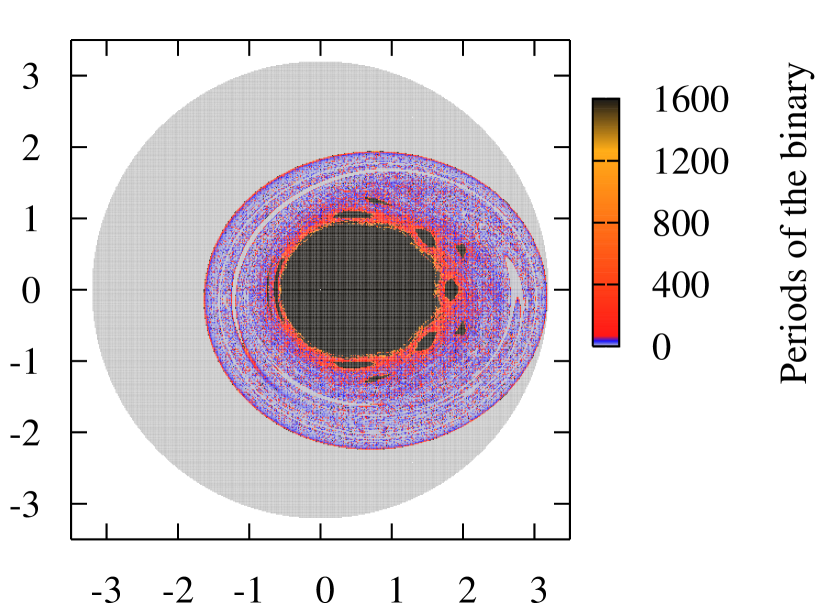
Figure 2: Survival time of orbits of the Sitnikov problem with initial conditions in the circle whose radius is given by (8). Each initial condition is plotted in polar coordinates where the radial argument is determined by the initial velocity and the angular argument is determined by $t_{0}$. The colour associated with each point indicates the number of periods of the binary before escape was determined.

Figure 2 shows the complement of the region defined by (8). A grid of initial conditions was chosen inside the disk and iterated forward using the Bulirsch-Stoer method (Press et al. (1992)) for either 10000 time units or until the escape criterion was satisfied. The colour associated with each initial condition represents the number of periods of the binary before $m_{3}$ either satisfied the escape criterion, or the numerical integration algorithm reached its maximum time. The outer grey region represents initial conditions in which the escape criterion was satisfied before the mass returned to the plane of motion of the binary. The inner black regions correspond to initial conditions whose orbits remain bounded.

2.3 Results

To demonstrate a relationship between the survival time and the Lyapunov time for the Sitnikov problem, 10000 initial conditions where chosen in the region described in section 2.2. The Bulirsch-Stoer method (Press et al., 1992) was chosen as the numerical integrator with a relative tolerance of $10^{-12}$. We integrated each initial condition simultaneously with the variational equations for $100000$ time units or until the solution satisfied the escape criterion. If the solution failed to satisfy the escape criterion within the time limit given to the integrator it was not considered in the results. This is because there is a large area of bounded motion, approximately the black regions in Figure 2, which never escape.

Figure 3 displays the $(t_{l},t_{d})$ scatter diagram in logarithmic scale for $\varepsilon=0.61$. As in Mikkola & Tanikawa (2007), the range of $t_{l}$ is divided into 50 intervals each containing an equal number of points. The dashed curve in Figure 3 displays the median of the survival time, $t_{d}$, in each of the 50 intervals. Comparing this plot to Figure 3 in Mikkola & Tanikawa (2007) we note some similarities. First, for small $t_{l}$ the median curve is steeper compared to larger $t_{l}$ values. Secondly, the density of the scatter points becomes smaller as $t_{l}$ increases. Finally, for small $t_{d}$ the scatter plot has horizontal band-like structures. In Figure 4 we re-plot the median curve in Figure 3 and approximate the median curve with (1) on two separate $t_{l}$ intervals. For $1<t_{l}<6$ we find that (1) approximates the curve with $\beta=2.5$. For $t_{l}>6$ we find that (1) approximates the data with $\beta=1.1$.

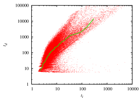
Figure 3: The scatter diagram of the survival time, $t_{d}$, and the Lyapunov time, $t_{l}$, for the Sitnikov problem where the eccentricity of the binary is $\varepsilon=0.61$. The dashed line is a median curve such that at any position along the curve there are an equal number of scatter points above and below the line.

Figure 4: The solid curve is the median curve shown in Figure 3. The two dashed lines represent the power law relationship (1) on different time intervals. For $1<t_{l}<6)$ we find that $\beta\approx 2.5$ best approximates the data. For $t_{l}>6$ we find that $\beta\approx 1.1$ works better.

2.4 Perturbations caused by large eccentricities

Of the systems studied by Mikkola & Tanikawa (2007), in particular the free-fall 3-body problem, the change in energy of the escaping body can vary widely depending on the interaction with the resulting binary system. This can be modelled in the Sitnikov problem by increasing the eccentricity of the binary.

Figure 5: The median $(t_{l},t_{d})$ curve for varying eccentricities of the Sitnikov problem.

Figure 5 represents the median curves for a series of experiments in which the eccentricity of the binary system in the Sitnikov problem is varied. One distinguishing feature in this figure is the increasing prominence of a two part power law relationship between the survival time and the Lyapunov time as the eccentricity increases. Interestingly, the minimum Lyapunov and survival times also decrease as the eccentricity increases.

In summary, by increasing the eccentricity of the Sitnikov problem we can cause large perturbations to the energy of $m_{3}$ and for $\varepsilon$ large enough the two-part power law becomes more prominent. An explanation for the different power laws between small and large $t_{l}$ is still needed. To help provide further theoretical explanations for the relationship we can turn to an approximate Poincaré map for the Sitnikov problem derived in Urminsky (2008b).

3 Approximate Poincaré map

The plane which corresponds to $z=0$ is a natural choice for a surface of section (SOS) on which to study escape with the Sitnikov problem. On the SOS we can consider a map $\phi:(v_{0},t_{0})\rightarrow(v_{1},t_{1})$ which takes $m_{3}$ from one crossing of the SOS to the next crossing. If $m_{3}$ is on the SOS at time $t_{0}$, $\phi$ is a map which brings $v_{0}=\dot{z}(t_{0})$ to time $t_{1}>t_{0}$ where $v_{1}=\dot{z}(t_{1})$ and $z(t_{1})=0$. Moser (1973) shows that there exists a real analytic simple closed curve in $\mathbb{R}^{2}$ in whose interior, $D_{0}$, the mapping $\phi$ is defined. In addition, $\phi$ maps $D_{0}$ onto a domain $D_{1}$ and for $\epsilon>0$ the boundary curves for $D_{0}$ and $D_{1}$ intersect transversally. Any point not in $D_{0}$ is said to escape.

Capturing the dynamics of the map $\phi$ can provide insights into the relationship between $t_{l}$ and $t_{d}$. To do this, we consider the following symplectic map which approximates $\phi$ (Urminsky, 2008b), including the approximation (4), from one crossing of the SOS at time $t_{0}$ to the next crossing at time $t_{1}$ given by $\Phi:(t_{0},E_{0})\rightarrow(t_{1},E_{1})$, where

$$\begin{array}[]{lcl}E_{1/2}&=&E_{0}+a\cos\left(t_{0}\right)+b\sin\left(t_{0}\right)\\ t_{1/2}&=&t_{0}+\alpha\left(-E_{1/2}\right)^{-3/2}\\ t_{1}&=&t_{1/2}+\alpha\left(-E_{1/2}\right)^{-3/2}\\ E_{1}&=&E_{1/2}-a\cos\left(t_{1}\right)+b\sin\left(t_{1}\right),\end{array}$$ (9)

and $a$, $b$ and $\alpha$ are constants. The quantities $t_{1/2}$ and $E_{1/2}$ are the time and energy values of $m_{3}$, respectively, when $m_{3}$ reaches a local maximum distance from the SOS with $\dot{z}(t_{1/2})=0$. The map is derived by approximating the change in energy of $m_{3}$ on two time intervals in which we approximate its orbit by an orbit which escapes parabolically. The first time interval $(t_{0},t_{1/2})$ corresponds to $m_{3}$ moving away from the SOS. The second time interval $(t_{1/2},t_{1})$ corresponds to the period in which $m_{3}$ returns to the SOS. It is clear that the change in energy is periodic in $t_{0}$ and the trigonometric terms in (9) can be thought of as a lowest order Fourier approximation to this change. The change in time is approximated by Keplerian motion over each time interval which means, for the chosen units, $\alpha=\pi/(2\sqrt{2})$. The map can be generalized as the iterative map $\Phi:(t_{n},E_{n})\rightarrow(t_{n+1},E_{n+1})$ and the constants $a$ and $b$ are approximately proportional to $\varepsilon$ with

$$\begin{array}[]{rcl}a&\approx&0.599\;\;\varepsilon/4\\ b&\approx&2.029\;\;\varepsilon/4.\end{array}$$ (10)

Sometimes it is more useful to write (9) in the form

$$\begin{array}[]{rcl}t_{n}&=&t_{n-1}+2\alpha(-X_{n-1})^{-3/2}\\ X_{n}&=&X_{n-1}+2b\sin(t_{n})\end{array}$$ (11)

for $n=1,2,3...$ where $X_{0}=E_{1/2}=E_{0}+a\cos(t_{0})+b\sin(t_{0})$, and generally $X_{n}=E_{n+1/2}$.

3.1 Initial conditions

Analogous to Moser’s $D_{0}$ and $D_{1}$ for (2), we can define an open domain $U_{0}$ for which $\Phi$ is defined which is mapped into an open region $U_{1}$. Since time enters into the change in energy with period $2\pi$, and we can transform energy values into velocity values by (3), we can consider $U_{0}$ in polar coordinates where the angular argument is determined by $t$ and the radial argument is determined by $v$. An upper bound on allowable energy values in $U_{0}$ is given by

$$E^{f}(t)=-a\cos\left(t\right)-a\sin\left(t\right),$$ (12)

for $t\in[0,2\pi]$ which corresponds to $E_{1/2}=0$ for which the map is undefined. All points in

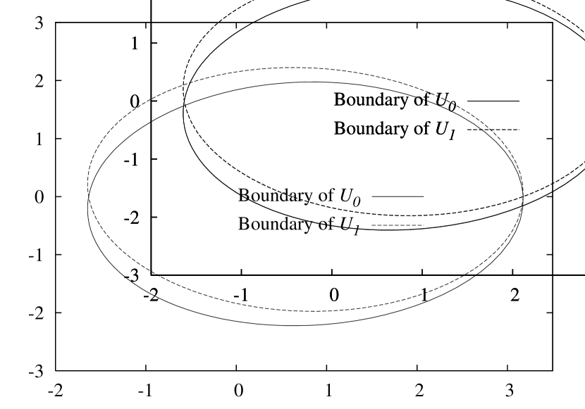
Figure 6: The boundaries $\partial U_{0}$ and $\partial U_{1}$ for the regions $U0$ and $U_{1}$ for $\varepsilon=0.61$.

$U_{0}$ get mapped to the open set $U_{1}$ whose boundary, $\partial U_{1}$, is defined by

$$E^{b}(t)=-a\cos\left(t\right)+b\sin\left(t\right),$$ (13)

for $t\in[0,2\pi]$. The boundaries $\partial U_{0}$ and $\partial U_{1}$ are depicted in Figure 6. Allowable energy values in $U_{0}$ at time $t$ satisfy $E<E^{f}(t)$. To satisfy the physical constraints of the Sitnikov problem, energy values in the domain $U_{0}$ are also bounded from below. From (3), energy values on the SOS must satisfy

$$E+\frac{1}{r(t)}\geq 0.$$ (14)

It has been shown by Urminsky (2008b), that the dynamics of orbits with initial conditions in $U_{0}$ for the map $\Phi$ are similar to the dynamics of orbits with initial conditions in $D_{0}$ for the map $\phi$. More specifically, it was shown that the map $\Phi$ satisfies lemmas similar to those proved by Moser (1973) which prove the existence of a set $\Lambda\in U_{0}$ on which the dynamics are topologically equivalent to the shift map on the set of bi-infinite sequences.

Initial conditions in $U_{0}$ can be iterated forwards using (9) until the resulting orbits take on energy and time values which are outside the domain $U_{0}$. A comparison of the Poincaré map $\phi$ and the approximate Poincaré map $\Phi$ can be found in Urminsky (2008a) in which regions of initial values on the SOS are delineated by the number of excursions from the SOS an orbit makes before escaping.

3.2 Definitions

For a given orbit $\mathcal{Z}=\{(t_{i},E_{i})\}_{i=0}^{N}$ computed by $\Phi$, where $N$ is the number of excursions from the SOS before $m_{3}$ escapes, the survival time is defined to be $t_{d}=t_{N}-t_{0}$. The growth of the logarithm of the solutions to the variational equations for the orbit $\mathcal{Z}$ is approximated by,

$$\ln|\delta\mathbf{Z}_{N}|\approx\sum_{i=0}^{N}\ln\left|\mathbf{w}_{i}\right|,$$ (15)

where $\mathbf{Z}_{N}=(t_{N},E_{N})$ and $\mathbf{w}_{i}$ is determined by,

$$\mathbf{w}_{i}=\mathbf{J}_{i-1}\frac{\mathbf{w}_{i-1}}{\left|\mathbf{w}_{i-1}\right|},\;\;\;\mbox{for}\;\;i=1,...,N,$$ (16)

in which $|\mathbf{w}_{0}|=1$ is chosen at random and $\mathbf{J}_{i}$ is the Jacobian of $\Phi$ at time step $i$. After a few iterations $\mathbf{w}_{i}$ is aligned with the unstable direction associated with the solution at the $i$th time step. In a similar way to equation (7), we can express the relationship between $t_{d}$ and $t_{l}$ as,

$$t_{l}\approx\frac{t_{d}}{\displaystyle\sum_{i=0}^{N}\ln\left|\mathbf{w}_{i}\right|}.$$ (17)

3.3 Numerical Results

$10000$ random uniformly distributed initial conditions were chosen in $U_{0}$ such that, when iterated using equation (9), they escaped within $1000$ iterations. If they failed to escape we did not include them in the calculations as there are regions of initial conditions in $U_{0}$ for which the corresponding orbits never escape. While calculating the orbit we simultaneously compute (15) so as to determine the Lyapunov time by equation (17). Figure 7 shows the $(t_{l},t_{d})$ scatter plot where the dashed line represents the median curve associated with the scatter plot.

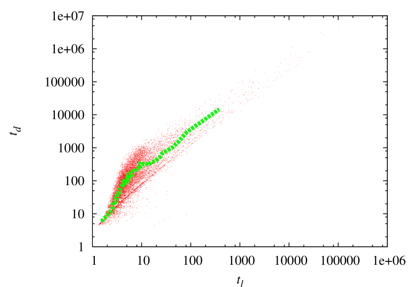
Figure 7: The $(t_{l},t_{d})$ scatter plot for 10000 uniformly distributed initial conditions in the domain of the map $\Phi$ for $\varepsilon=0.61$. The dashed line is the median curve associated with the scatter plot.

Figure 8: Two part power law relationship for 100000 initial conditions for the map ($\varepsilon=0.61$)

Notice that the horizontal spread of the scatter plot for small time values found in Figure 3 is present in Figure 7. In addition, the density of the plotted points decreases as $t_{l}$ increases.

In Figure 8 we plot the median curve for the $(t_{l},t_{d})$ scatter plot for 100000 uniformly distributed initial conditions for $\varepsilon=0.61$. Again, there appears to be a two-part power law relationship for $t_{l}$. The power law (1) with $\beta=2.5$ approximately fits the median curve on the interval $1<t_{l}<9$, whereas a power law with $\beta=1.07$ fits better for $t_{l}>9$. Figure 9 shows the median curves for various eccentricities of the binary. As in Figure 5, as the eccentricity of the binary increases, the two-part power law become apparent.

Figure 9: Median curves for the map $\Phi$ for varying eccentricity values.

Figure 10: The median curve on the interval containing 90 per cent of the points in Figure 8. On this interval a power law relationship with $\beta\approx 1.1$ fits the data best.

Finally, we consider the time interval $4.4<t_{l}<129.7$ which contains 90 per cent of the scatter points in Figure 7. This interval was chosen such that 5 per cent of the scatter points were in the region $t_{l}<4.4$ and 5 per cent of the points were in the region $t_{l}>129.7$. It was found that in this region a power law relationship with $\beta\approx 1.1$ best fitted the median curve (Figure 10). This contrasts with the result in Mikkola & Tanikawa (2007) for the general 3-body problem where it was found that a power law with $\beta\approx 1.8$ roughly fits 90 per cent of the data on an interval $.94<t_{l}<35.2$. Since the data in Figure 10 is distributed over a larger interval, the data for larger $t_{l}$ values dominates the approximation and the smaller power law approximation best fits the data. We shall demonstrate in section 4 that the distribution of $t_{d}$ for the map is different than that found for the general 3-body problem which may account for the discrepancy between the two results.

3.4 Delineating the region corresponding to escape after one excursion

Initial conditions along the boundary $\partial U_{0}$ defined by (12) lead to $E_{1/2}=0$. From equation (9), we can see that these initial conditions lead to a time $t_{1/2}$ which is undefined. Initial conditions on $E^{f}(t)$ for $t\in(0,\pi)$ are contained in the set $D_{1}$ and so are in the domain of the inverse map $\Phi^{-1}$. Iterating these initial conditions backwards once gives the boundary of the region, $B_{1}$, corresponding to penultimate crossings of the SOS before escape. The boundary of $B_{1}$ can be shown to be given parametrically by,

$$\begin{array}[]{rcl}t_{*}&=&t-2\alpha(2b\sin(t))^{-3/2}\\ E_{*}&=&-2b\sin(t)-a\cos(t_{*})-b\sin(t_{*}).\end{array}$$ (18)

This boundary is shown in Figure 11 using polar co-ordinates where the angular argument is time and the radial argument is the velocity of $m_{3}$ obtained from (3).

Figure 11: The boundary of the region $B_{1}$.

Iterating initial values on this boundary forward in time using (9) leads to energy values $E_{3/2}=0$ and from equation (9) we get,

$$E_{3/2}=E_{1/2}+2b\sin(t_{1})=0.$$ (19)

Writing (19) in terms of $E_{0}$ and $t_{0}$ and rearranging gives,

$$\begin{array}[]{l}E_{0}+a\cos(t_{0})+b\sin(t_{0})=\\ \;\;\;-2b\sin\left(t_{0}+2\alpha(-E_{0}-a\cos(t_{0})-b\sin(t_{0}))^{-3/2}\right).\end{array}$$ (20)

As the boundary of $B_{1}$ spirals inside $U_{0}$ (Figure 11) it approaches the boundary $\partial U_{0}$. Consider $E_{0}$ values on the boundary of $B_{1}$ for a fixed $t_{0}$. Define

$$\theta=2\alpha\left(-E_{0}-a\cos(t_{0})-b\sin(t_{0})\right)^{-3/2}$$ (21)

and note that $\theta\rightarrow\infty$ as $E_{0}\rightarrow E^{f}(t_{0})$. Using equation (21) we can re-write (20) as

$$-\left(\frac{\theta}{2\alpha}\right)^{-2/3}=2b\sin(t_{0}+\theta),$$ (22)

and as $\theta\rightarrow\infty$ solutions to (22) are asymptotically approximated by,

$$\theta+t_{0}\approx k\pi,$$ (23)

for large $k\in\mathbb{Z}$. Substituting equation (21) into (23) we can obtain the approximation for the energy values on the boundary of $B_{1}$

$$E_{0}^{k}\approx-\left(\frac{k\pi-t_{0}}{2\alpha}\right)-a\cos(t_{0})-b\sin(t_{0}),$$ (24)

for large $k\in\mathbb{Z}$. Initial conditions on $B_{1}$ survive only one iteration of the map $\Phi$. Substituting (24) into (9) gives the survival time for orbits of initial conditions on the boundary of $B_{1}$ as

$$t_{d}=t_{1}-t_{0}\approx 2\alpha\left(\left(\frac{k\pi-t_{0}}{2\alpha}\right)^{-2/3}\right)^{-3/2}=k\pi-t_{0}.$$ (25)

3.5 A functional relationship between $t_{l}$ and $t_{d}$

To derive a functional relationship between $t_{l}$ and $t_{d}$, we consider initial conditions on the boundary of $B_{1}$ for a fixed $t_{0}$. For $t_{0}=\pi/2$, initial conditions on $\partial B_{1}$ are approximated by,

$$\begin{array}[]{lcl}t_{0}&=&\pi/2,\\ E_{0}&=&-\left(\displaystyle\frac{(k-1/2)\pi}{2\alpha}\right)^{-2/3}-b,\end{array}$$ (26)

for large $k\in\mathbb{Z}$. Using the initial conditions (26) and the corresponding survival time given by (25), we can compute the Lyapunov time $t_{l}$ from (17) for a given initial $|\mathbf{w}_{0}|=1$. For long lived orbits it may be assumed that $\mathbf{w}_{k}$ will normally become aligned with the unstable direction after only a few iterations. For initial conditions along $\partial B_{1}$ on the other hand, this assumption is invalid since the orbit escapes after only one excursion. The choice of $\mathbf{w}_{0}$ has an important role in determining the growth of $|\delta\mathbf{Z}_{1}|$ as it may not necessarily be aligned with the most unstable direction.

The vector $\mathbf{w}_{0}$ should be chosen so as to give the largest $|\delta\mathbf{Z}_{1}|$ possible. Choosing $\mathbf{w}_{0}$ in this way has the effect of making $t_{l}$ small. Figure 12 shows the $(t_{l},t_{d})$ scatter plot for initial values given by (18) for various choices of $\mathbf{w}_{0}$. It was found that the vector $\mathbf{w}_{0}=[0,1]$ maximizes $\ln|\delta\mathbf{Z}_{1}|$ and ensures that $\ln|\delta\mathbf{Z}_{1}|>0$ for orbits of initial conditions on the boundary of $B_{1}$.

Figure 12: The $(t_{l},t_{d})$ scatter plot for orbits with initial values on the boundary of $B_{1}$ for varying initial vector $\mathbf{w}_{0}$ ( $\varepsilon=0.61$).

For initial conditions in $B_{1}$, the contribution of the denominator in equation (17) is $\ln|\mathbf{w}_{1}|$ since $|\mathbf{w}_{0}|=1$. For initial conditions (26) with initial vector $\mathbf{w}_{0}=[0,1]$ we can compute $|\mathbf{w}_{1}|$ from equation (16) to obtain

$$\begin{array}[]{l}|\mathbf{w}_{1}|^{2}=9\alpha\left(\displaystyle\frac{(k-1/2)\pi}{2\alpha}\right)^{10/3}\\ \;\;\;\;\;\;\;\;\;\;\;\;\;+\left(1+3b\alpha(-1)^{k}\left(\displaystyle\frac{(k-1/2)\pi}{2\alpha}\right)^{5/3}\right)^{2}.\end{array}$$ (27)

For large $k$ we have

$$|\mathbf{w}_{1}|\simeq(k\pi)^{5/3},$$ (28)

and hence, for orbits of initial values (26),

$$\ln|\mathbf{w}_{1}|\simeq 5\ln(k\pi)/3.$$ (29)

Substituting this result into (17), we find that the Lyapunov time for initial values on the boundary of $B_{1}$ behaves like,

$$t_{l}\simeq\frac{3k\pi}{5\ln(k\pi)}\;\;\mbox{for large}\;\;k\in\mathbb{Z},$$ (30)

where the survival time is determined by (25). Since $t_{d}\sim k\pi$ we can rewrite (30) as

$$t_{l}\simeq\frac{3t_{d}}{5\ln(t_{d})},$$ (31)

which for large $t_{d}$ is of order $t_{d}/\ln(t_{d})$.

Figure 13: Various approximations to the scatter $(t_{l},t_{d})$ plot of orbits which escape after one excursion from the SOS.

Figure 13 shows various approximations to the scatter $(t_{l},t_{d})$ plot (represented by the solid line) for orbits which escape after one excursion from the SOS. A best fit for a curve in the form of the power law relationship (1) is shown by the long dashed line where $\beta=1.07$. This curve does not fit the scatter plot for small or large $t_{l}$ very well. The dotted curve represents the function $t_{l}=t_{d}/\ln|\mathbf{w}_{1}|$, for $|\mathbf{w}_{1}|$ given by (27), which approximates the scatter plot better than the power law relationship. Finally, the small dashed curve is the function $t_{l}=3t_{d}/(5\ln(t_{d})$ which is only a slightly better approximation to the scatter plot for small $t_{d}$, but a much simpler one.

3.6 A general functional relationship between $t_{l}$ and $t_{d}$

Figure 14: The solid line is the median curve in Figure 8 for $\varepsilon=0.61$. The dashed line is the relationship (35) with $\rho=0.16$ and $\nu=.12$.

Now consider the orbits which escape after two excursions from the SOS. From equation (17) the Lyapunov time can be approximated by,

$$t_{l}\approx\frac{t_{d}}{\ln|\mathbf{w}_{1}|+\ln|\mathbf{w}_{2}|}.$$ (32)

Following the result of the previous section, we assume that each term in the denominator is proportional to the log of the time spent between successive crossings of the SOS. For escape after two crossings these sum to $t_{d}$ and we take the two contributions to be $\ln(ft_{d})$ and $\ln((1-f)t_{d})$ where $0<f<1$, i.e.

$$t_{l}\sim\frac{t_{d}}{\ln\left(ft_{d}\right)+\ln\left((1-f)t_{d}\right)}.$$ (33)

Re-arranging (33) we get

$$t_{l}\sim\frac{t_{d}}{\ln\left(f\left(1-f\right)t_{d}^{2}\right)}.$$ (34)

This relationship suggests fitting the data to curves which look like,

$$t_{l}=\rho\frac{t_{d}}{\ln\left(\nu t_{d}\right)}$$ (35)

where $\rho$ and $\nu$ are constants. In fact, adding successive iterations produces a similar result so we take (35) as a general relationship and try to vary $\rho$ and $\nu$ to optimize a fit to the data. Figure 14 shows the median curve (red solid curve) for 100000 initial values which escape within 1000 iterations of the map for $\varepsilon=0.61$. We were able to approximately fit the data with a function like (35) where $\rho=0.16$ and $\nu=.12$.

4 Distributions

Now we look at the distributions of the various quantities studied so far and compare them to the results for the general 3-body problem. In the numerical experiments for the general 3-body problem in Mikkola & Tanikawa (2007), the authors fit the marginal distribution of $t_{d}$ (for large values of $t_{d}$) and large values of the ratio $Z=t_{d}/t_{l}$ to exponential probability density functions, finding that

$$\psi(t_{d}) \approx \alpha\exp(-\alpha t_{d}),\;\;\alpha=1/250,$$ (36)

$$\psi(Z) \approx \beta\exp(-\beta Z),\;\;\beta=1/45.$$ (37)

The probability density for $t_{l}$ in the general 3-body problem was obtained numerically and a theoretical explanation was given in Mikkola & Tanikawa (2007) as follows. The authors assume that $t_{d}$ and $Z$ are independent variables and so the marginal probability density function, $\psi(t_{l})$, can be determined via

$$\begin{array}[]{rcl}\psi(t_{l})&\approx&\displaystyle\int\delta(t_{l}-t_{d}/Z)\psi(t_{d})\psi(Z)dt_{d}dZ,\\ &=&\alpha\beta/(\alpha t_{l}+\beta)^{2}.\end{array}$$ (38)

Their numerical results do not quite match up with (38), but the authors did fit their data with a function proportional to $t_{l}^{-2}$. The problem may be that equation (38) assumes that $t_{d}$ and $Z$ are independent variables. This does not seem to be likely considering Figure 3. It may be that, while the distributions provide satisfactory fits, an expression like (38) may not always be true.

Figure 15: The solid curve is the probability density of $t_{d}$ for the numerical results with $\varepsilon=0.61$. The dashed curve was found to be the best approximation of the stated form to the numerical results.

Figure 16: The solid curve is the probability density of $t_{d}$ for the numerical results with $\varepsilon=0.61$ for small $t_{d}$. The dashed curve was found to be the best approximation of the stated form to the numerical results.

Orbits computed with the map $\Phi$ also possess a similar power law relationship between $t_{d}$ and $t_{l}$, for large enough eccentricities, to those found in the general 3-body problem and the Sitnikov problem. The map may provide some insights into the distributions for $t_{d}$, $Z$ and $t_{l}$. Figure 15 shows the numerical results for the distribution of $t_{d}$ values for the map $\Phi$ where $\varepsilon=0.61$. The $t_{d}$ values are binned into intervals of length 200 along the whole range of $0\leq t_{d}\leq 70000$ and the number of $t_{d}$ values in each bin is counted and divided by the total number of initial conditions. It was found that a probability density function

$$\Psi(t_{d})\approx a_{1}b_{1}/(a_{1}t_{d}+b_{1})^{2},$$ (39)

where $a_{1}=0.48$ and $b_{1}=216.3$ best represents the data in Figure 15. Figure 16 shows the results for $t_{d}<1000$ which demonstrates that this is a good approximation for small $t_{d}$. Similarly, it was found that a probability density function for $Z$ which fits the numerical data satisfactorily is given by

$$\Psi(Z)\approx a_{2}b_{2}/(a_{2}Z+b_{2})^{2},$$ (40)

where $a_{2}=10.35$ and $b_{2}=160.71$ as shown in Figure 17.

Figure 17: The solid curve is the probability density of $Z$ for the numerical results with $\varepsilon=0.61$. The dashed curve was found to be the best approximation of the stated form to the numerical results.

Figure 18: The solid curve shows the probability density of $t_{l}$ for the numerical experiments with $\varepsilon=0.61$.

Figure 19: The solid curve shows the probability density of $t_{l}$ for the numerical experiments with $\varepsilon=0.61$ for small $t_{l}$.

The marginal probability density functions for $t_{d}$ and $Z$ are quite different to those for for the general 3-body problem. This means that the predicted density function (38) may not necessarily hold for the map. Proceeding as in (38), assuming the variables $t_{d}$ and $Z$ are independent, the density function for $t_{l}$ can be determined by,

$$\begin{array}[]{rcl}\Psi(t_{l})&=&\displaystyle\int\delta(t_{l}-t_{d}/Z)\Psi(t_{d})\Psi(t_{l})dt_{d}\;dt_{l}\\ &=&-\displaystyle\frac{2b_{1}a_{2}\ln\left(\displaystyle\frac{b_{1}}{a_{1}t_{l}}\right)}{(-a_{2}b_{1}+b_{2}a_{1}t_{l})^{3}}-\frac{1+\ln\left(\displaystyle\frac{b_{1}}{a_{1}t_{l}}\right)}{(-a_{2}b_{1}+b_{2}a_{1}t_{l})^{2}}\\ &&+\displaystyle\frac{2a_{1}b_{2}t_{l}\ln\left(\displaystyle\frac{b_{2}}{a_{2}}\right)}{(-a_{2}b_{1}+b_{2}a_{1}t_{l})^{3}}-\displaystyle\frac{1+\ln\left(\displaystyle\frac{b_{2}}{a_{2}}\right)}{(-a_{2}b_{1}+b_{2}a_{1}t_{l})^{2}}.\end{array}$$ (41)

Figure 18 shows the numerical results for the map $\Phi$ for $\varepsilon=0.61$. The solid curve shows the data from the experiments, and the medium dashed curve is the predicted curve (41) where $g(t_{l})=\Psi(t_{l})$. Note that the curve does not quite fit the data from the experiments for small $t_{l}$ (Figure 19). The data was then fitted to a curve of the form,

$$\Psi(t_{l})\approx ab/(at_{d}+b)^{2},\;\;\mbox{where}\;\;a=0.53,\;b=2.75,$$ (42)

shown by the short dashed curve. Again, this failed to fit the data for small $t_{l}$. It was noted that the data is better approximated by the curve,

$$f(t_{l})=32/t_{l}^{2}.$$ (43)

Interestingly, this is a similar function to that which fits the numerical results for the general 3-body problem. This suggests that the probability distribution associated with the Lyapunov time may not necessarily be the result of the probability distribution of survival times and the probability distribution of the variable $Z$.

5 Conclusions

One of the results of this investigation is demonstrating a relationship between the Lyapunov time and the survival time for the Sitnikov problem which is similar to that for the general 3-body problem found in Mikkola & Tanikawa (2007). This is surprising as the Sitnikov problem is rather different compared to the 3-body systems discussed in Mikkola & Tanikawa (2007). With the use of an approximate Poincaré map we were able to delineate regions of escape on a surface of section so as to construct initial conditions for the map. By studying the relationship between the Lyapunov time and the survival time with initial conditions in distinct escape regions, we were able to analytically obtain a new functional relationship between $t_{l}$ and $t_{d}$ given by $t_{l}=\rho t_{d}/\ln(\nu t_{d})$ where $\rho$ and $\nu$ are constants. As the $(t_{l},t_{d})$ scatter plots for the Sitnikov problem are similar to the $(t_{l},t_{d})$ scatter plots for the general 3-body problem, we conjecture that the new functional relationship between $t_{l}$ and $t_{d}$ presented above may also be valid for the general 3-body problem.

Interestingly, the marginal distributions for the quantities $t_{d}$ and $Z$ were found to be different than for the general 3-body problem. The reason for this is not known although it may just be that in this study we considered the entirety of the numerical results and not just large values. Treating $t_{d}$ and $Z$ as independent variables, we were able to derive a marginal distribution for $t_{l}$ which did not quite capture the numerical results. It seems unlikely though that $t_{d}$ and $Z$ are independent quantities which may be why the theoretical predicted distribution $\Psi(t_{l})$ did not quite match the numerical results. Interestingly, as for the general 3-body problem, it was found that a function proportional to $t_{l}^{-2}$ fits the numerical distribution of $t_{l}$ well. This may point to a more general property which may be valid for 3-body problems which experience large perturbations to an escaping mass.

References

- Lecar et al. (1992) Lecar M., Franklin F., Murison M., 1992, AJ, 104, 1230
- Lecar et al. (1992b) Lecar M., Franklin F., Soper P., 1992, Icarus, 96
- Levison & Duncan (1993) Levison H., Duncan M.J., 1993,Astrophys. J., Lett., 406, L35
- Mikkola & Tanikawa (2007) Mikkola S., Tanikawa K., 2007, MNRAS, 379, L21
- Morbidelli & Froeschlé (1996) Morbidelli A., Froeschlé C., 1996, AJ, 108, 2323
- Moser (1973) Moser J., 1973, Stable and Random Motions in Dynamical Systems, Princeton U. Press, Princeton
- Murison et al. (1994) Murison M.A., Lecar M., Franklin F.A., 1994,AJ, 108, 6
- Murray & Holman (1997) Murray N., Holman M.,1997,AJ, 114, 1246
- Press et al. (1992) Press W.H., Teukolsky S.A., Vetterling W.T., Flannery B.P., Numerical Recipes in C, The Art of Scientific Computing, Cambridge U. Press
- Soper et al. (1990) Soper P., Franklin F., Lecar M., 1990, Icarus,87
- Urminsky (2008a) Urminsky D.J., 2008a, IAUS, 246, 235
- Urminsky (2008b) Urminsky D.J., 2008b, PhD thesis, University of Edinburgh