Slow Relaxation and Equilibrium Dynamics in a 2 D Coulomb Glass: Demonstration of Stretched Exponential Energy Correlations

Abstract

We have simulated energy relaxation and equilibrium dynamics in Coulomb Glasses using the random energy lattice model. We show that in a temperature range where the Coulomb Gap is already well developed, ($T=0.03-0.1$) the system still relaxes to an equilibrium behavior within the simulation time scale. For all temperatures $T$, the relaxation is slower than exponential. Analyzing the energy correlations of the system at equilibrium $C(\tau)$, we find a stretched exponential behavior, $C(\tau)=e^{-(\tau/\tau_{0})^{\gamma}}$. We study the temperature dependence of $\tau_{0}$ and $\gamma$. $\tau_{0}$ is shown to increase faster than exponentially with decreasing $T$. $\gamma$ is proportional to $T$ at low temperature, and approaches unity for high temperature. We define a time $\tau_{\gamma}$ from these stretched exponential correlations, and show that this time corresponds well with the time required to reach equilibrium. From our data it is not possible to determine whether $\tau_{\gamma}$ diverges at any finite temperature, indicating a glass transition, or whether this divergence happens at zero temperature. While the time dependence of the system energy can be well fitted by a random walker in a harmonic potential for high temperatures ($T=10$), this simple model fails to describe the long time scales observed at lower temperatures. Instead we present an interpretation of the configuration space as a structure with fractal properties, and the time evolution as a random walk on this fractal-like structure.

I Introduction

In a doped semiconductor at low temperature, electron transport can be dominated by variable range hopping of localized electrons.Mott If the active impurities are sufficiently close, the Coulomb interaction between the localized electrons will give an important contribution to the disorder of the energy levels. Such a system is known as a Coulomb Glass, where the term ’glass’ is due to the many features it shares with other glasses, including slow dynamics and aging, and short distance correlations combined with long range disorder.

Coulomb Glasses have been studied extensively both numerically and analytically. Among the top theoretical results describing the model is the derivation by Efros and Shklovskii of the ’Coulomb Gap’, a gap in the distribution of single electron state energies at any given time.EfrosShklovskii

Among the most interesting experimental results we would like to mention the demonstration of memory effects in the conductivity experiments performed by Ovadyahu et al.,Ovadyahu and the large $1/f$-noise increase related to the metal-insulator transition observed by Kar et al.Kar

The first simulations trying to model the Coulomb Glass were performed by Kurosawa.Kurosawa Later several groups have studied various parameter spaces, using very different approaches. In all approaches we have found, the defects have been modeled as static sites, with the electrons jumping from site to site. The number of electrons is usually chosen to be half that of the sites, reflecting a symmetry in states over and under the Fermi level.

The disorder of the system can be modeled in two different ways. First, one can choose to place the sites the electrons can jump between in a regular lattice, and introduce disorder through a local site energy. This means distances are functions of site index difference only, greatly reducing calculational effort. The second possibility is having sites of equal local site energy, and introducing disorder through the position of the sites. This gives the advantage of a symmetry in occupation numbers, changing the occupation of all states gives a state of the same energy, allowing a convenient definition of an order parameter.Davies The applicability of this order parameter has recently been disputed by Matulewski et al.,MATULEWSKI who claim that the long range interaction of the electrons leads to a system size dependence of the order parameter, and that the temperature where it goes to zero depends on the minimal inter-site distance allowed. It can be argued that positional disorder requires smaller system sizes for good statistics at low temperatures, as the energy disorder will lead to some sites “freezing out” and having fixed occupation probability. However, it is possible that the two models can give very different behavior, so the further study of both is definitely justified.

The most realistic model would be to study a 3D model. Still, many simulations, including ours, use a 2D model only. The advantage of this is that we can study systems of much larger linear dimension, which we assume to be important due to the long range nature of the Coulomb interaction.

Next, choice of temperature range greatly affects the choice of algorithm. For small systems at extremely low temperatures, it is possible to imagine that all configurations relevant for the dynamics can be mapped, and transitions between these calculated.DiazSanchez ; Pollak This allows studying the effect of transitions involving multiple simultaneous electron jumps. Increases in size and temperature rapidly makes this method impossible, even with the best future supercomputers. Fortunately, increasing temperature also reduces the role of multi-electron jumps,Pollak as a wider range of states is accessible.

At higher temperatures, Monte Carlo simulations have been performed in various ways, which can be divided in two groups. At high temperatures, the Metropolis algorithm of picking a possible jump and accepting it with a given probability is very efficient.Metropolis ; Tsigankov ; Kolton ; GrannanYu At lower temperatures, where only a small number of jumps are probable, one can calculate all possible jump rates, and accept one jump based on relative probabilities.MobiusThomas ; Ortuno ; Somoza Various optimizations and hybrids of these methods have also been used. Our simulations belong to the latter category, and includes some optimizations we have not seen elsewhere.

Our long term goal in starting this work is to study conductance in Coulomb Glasses, and in particular to try to demonstrate the interesting effects observed in experiments.Ovadyahu ; Kar In order to achieve this, we need to establish which model and parameter choice is appropriate. For example, Tsigankov et. al.Tsigankov argue that the variations in conductivity observed in Ovadyahu’s experiments can be reproduced for the random position model, but not for the lattice model, both at a temperature of $T=0.04$. Our results indicate that this may be due to the transition temperature for this kind of behavior being lower than $T=0.04$ for the lattice model, while it happens at a higher temperature for the position disorder. This demonstrates how insufficient charting of the parameter space may lead to wasted effort later. After surveying the literature, we have realized that there is not even agreement on whether there is a glass transition at any finite temperature for the lattice model in 2 dimensions.

In principle, we need a complete understanding of the roles of all the adjustable parameters; temperature, electron localization length, disorder strength, disorder type, time scale and system size. In the present paper, we have chosen to focus on the time scale of equilibration of the system. In this way give an upper temperature limit for when glassy effects can be observed, and estimate how the time scales of these effects change with temperature.

In the analysis of the data, we have been inspired by work on spin glasses, which show many of the same features as Coulomb glasses. This is a field which has been studied in much greater detail. We have based our analysis on work by Ogielski,Ogielski whose methods have been a powerful tool in understanding our results. We find that there are clear similarities in our results and those obtained for spin glasses. For example, we have found that the correlation function of the energy follows a stretched exponential behavior at long times, a result we have not seen in previous discussions on Coulomb Glasses.

However, neither the distance dependent interaction nor the charge conservation requirements found in Coulomb glasses have obvious parallels in the spin glass. This is reflected in the fact that the exponent we observe in the stretched exponential behaves differently from what has been reported for spin glasses.

II Model

We have used the standard 2D lattice model with Hamiltonian

$$\mathcal{H}=\sum_{i}U_{i}(n_{i}-\bar{n})+\frac{1}{2}\sum_{i,j}\frac{(n_{i}-\bar{n})(n_{j}-\bar{n})}{r_{i,j}}.$$ (1)

Here $\bar{n}$ is the average occupancy, $n_{i}=0,1$ is the occupancy of site $i$, and $r_{i,j}$ is the distance between sites $i$ and $j$. $U_{i}$ is the site occupancy energy of site $i$, drawn from a uniform distribution on the interval $[-U,U]$. All energies and temperatures are measured in units of the nearest neighbor Coulomb interaction $e^{2}/a$, where $a$ is the lattice constant and $e$ is the elementary charge.

We use periodic boundary conditions in both dimensions, and side lengths of $L$, forcing us to cut off the Coulomb interaction at the distance $L/2$. $N=L^{2}$ is the total number of sites. In all simulations presented here, we have used $U=1$, as this is standard in the literature. However, it should be noted that at this value of the disorder, the Coulomb Gap does not have the universal shape predicted by Efros and Shklovskii,EfrosShklovskii as shown in refs. MobiusRichterDrittler, ; Pikus, ; Glatz, . While this may be of importance for details in the temperature dependence of various quantities, we do not believe that it will significantly affect our results.

In order to calculate changes in the system energy $E$, we use the “single electron energy” $\epsilon_{i}$, defined by Efros and Shklovskii, the energy gained by adding an electron to an empty site, or required to remove the electron from an occupied site. It is given by

$$\epsilon_{i}=U_{i}+\sum_{j}\frac{(n_{j}-\bar{n})}{r_{i,j}}.$$ (2)

The change in system energy due to an electron hopping from site $i$ to site $j$ is then

$$\Delta E_{i\rightarrow j}=\epsilon_{j}-\epsilon_{i}-1/r_{i,j}.$$ (3)

The impurities are modeled as hydrogen-like states centered on the lattice sites, with a localization length $a_{l}$ chosen to be $2/3a$.

The relaxation has been performed by a modified Monte-Carlo simulation optimized for low temperatures, but still capable of handling high temperatures. A detailed description of the algorithm is given in appendix A, along with a discussion of the chosen parameters.

We follow Efros and ShklovskiiEfrosShklovskii and write the electron jump rate for the jump from the occupied site $i$ to the unoccupied site $j$ as

$$\Gamma_{i\rightarrow j}=t_{0}^{-1}e^{-2r_{i,j}/a_{l}}\frac{|\Delta E_{i\rightarrow j}|}{T_{0}}f(\Delta E_{i\rightarrow j}),$$ (4)

where for processes involving phonon emission,

$$f(\Delta E_{i\rightarrow j})=1+\frac{1}{e^{|\Delta E_{i\rightarrow j}|/T}-1},\qquad\Delta E_{i\rightarrow j}<0$$ (5)

while for phonon absorption

$$f(\Delta E_{i\rightarrow j})=\frac{1}{e^{\Delta E_{i\rightarrow j}/T}-1},\qquad\Delta E_{i\rightarrow j}>0.$$ (6)

We have made no estimates for the numbers $t_{0}$ and $T_{0}$, so for the plots showing a time scale, they should both be taken as unity. The time for one electron jump, $\Delta t$, is the inverse of the total rate

$$\Delta t=\frac{1}{\Gamma_{tot}},\qquad\Gamma_{tot}=\sum_{i\neq j}\Gamma_{i\rightarrow j}$$ (7)

This is the time during which, on average, one jump takes place. To get the correct noise spectrum at very short time scales, $\Delta t$ should have been drawn from a distribution with average $1/\Gamma_{tot}$, this we have ignored.

We have not seen any other simulations stating that they use the full expressions for the jump probability, most authors seem to use the low temperature limit of the expressions to reduce computational effort. Temperature in all equations is the phonon bath temperature.

III Results of relaxation

In order to study the temperature dependence of the relaxation process, all relaxations were started from the same random electron configuration, representing an infinite temperature and with the same realization of disorder. We then set the phonon bath to a given temperature, simulating a rapid quench. We follow the relaxation process by plotting the total system energy as function of time, as done by Ortuño et al Ortuno for the model with positional disorder. As shown in figure 1, the processes initially looks the same at all temperatures. This is because the system is still at some high energy and does not “feel” the differences in phonon temperature which are small compared to the initial infinite temperature of the system. In this regime, essentially all jumps reduce the total energy of the system.

Then, starting with the highest temperatures, one by one the systems seem to reach an equilibrium behavior, with the energy fluctuating around some average value. For all temperatures we observe that the relaxation is slower than exponential. For the lowest temperatures ($T\lesssim 0.02$) we are not able to reach the equilibrium state, and the system continues to relax to lower energies for our entire simulation time.

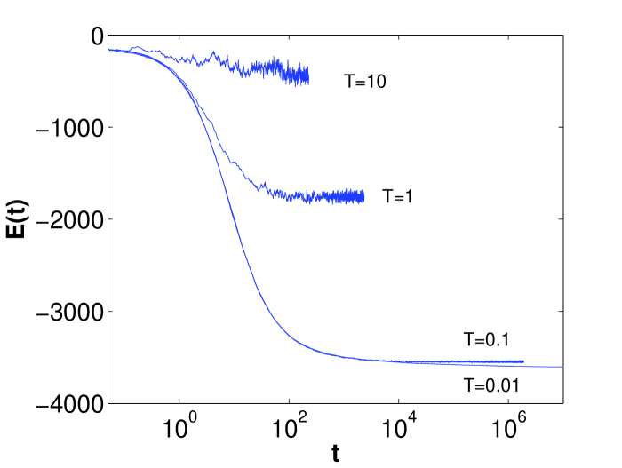
Figure 1: Plot of the relaxation from $T=\infty$ at temperatures $T=\{10,1,0.1,0.01\}$, the equilibrium energy decreases with $T$. We see that for $T=0.1$ we still get an equilibrium, while for $T=0.01$ or lower, equilibrium is not achieved at our time scale. Close-ups of the tails of the two lowest graphs are shown in Fig. 2

Zooming in on the different relaxation graphs, we can see significant qualitative differences, as shown in Fig. 2. At high temperatures where equilibrium is reached ($T\gtrsim 0.02$), we see something resembling a random walk in a confining potential (Fig. 2c). For $T=0.01$ (Fig. 2b) we see periods with something like a random walk around a central value, similar to the high temperature equilibrium case. At intervals this is interrupted by a sudden marked decrease in the energy, and the process continues with a lower mean energy. The periods of apparent equilibrium can be understood as some local equilibrium around a metastable local minimum of the energy and the steps correspond to the system crossing to a different local minimum. We have also observed steps that increase the energy, but they are usually smaller and less frequent, so that the long time average still is decreasing for the whole simulation period. For the lowest temperatures (Fig. 2a), we see the energy making small fluctuations from a clearly defined lowest level, which again decreases in clear steps. The steps are now much larger than the width of the distribution within one step. At these temperatures, the system actually finds the local minimal state and spends a considerable fraction of the time in this state. We believe that this is an effect of the finite size of our system, and that if we had increased the system size, the number of states accessible close to the local minimum would also increase. The system would then not so easily find its way to the local minimum, and we would get a picture similar to Fig. 2b even at the lowest temperatures. The nature and statistics of the steps are discussed in greater detail in appendix C.

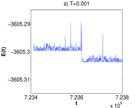
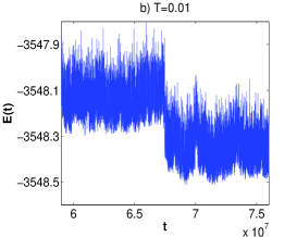
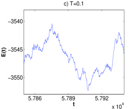
Figure 2: Close-up of the energy development at $T=\{0.001,0.1\}$, 500 jumps each, and $T=0.01$, 250000 jumps. $T=0.001$ shows a clear local minimum performing steps, $T=0.01$ has no sharp lower limit, but shows both steps and a tendency of differences in going up and down, while for $T=0.1$ there seems to be good symmetry around the mean and no steps can be identified. The width of the distribution is many times the energy of single jumps, which are of the order $T$

One can ask whether the equilibrium that we seem to observe at temperatures above $T=0.02$ really is a true equilibrium, or the system is still relaxing in energy, but so slowly that we are not able to see this in our simulations. In order to confirm that we have attained true equilibrium, we can initiate the system at a low energy. We have used two different ways of initiating the system. One is to relax the system at a lower temperature, and then increase the temperature. The other is to relax the system at zero temperature (using the algorithm described in ref. Glatz, , a less CPU-consuming procedure) a great number of times, and picking the configuration with the lowest energy as the starting energy for the Monte Carlo algorithm. Both of these were tested, giving the same result. As shown in Fig. 3, we see that even though we initiate the system at a low energy, it relaxes right up to the equilibrium energy range. We consider this as proof that true equilibrium was reached at temperatures $T\geq 0.03$. $T=0.03$ is the lowest temperature for which we have been able to achieve such a confirmation of equilibrium, simply because we have not found any state with $E$ lower than at the end of the $T=0.02$ simulation. Thus we have no low-energy starting point - at even lower temperature, the relaxation is so slow that we have not reached energies lower than those of the $T=0.02$ simulation.

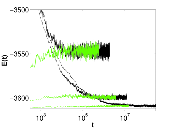
Figure 3: Plot of the relaxation from high and low energy starting points for T={0.03, 0.05, 0.1}. The straight line at the bottom shows the starting energy of the rising graph at $T=0.03$. For T=0.03 the graphs starting at high and low energy do not overlap fully because we have not continued the low-starting simulation for a sufficient number of steps. One can check that the average at the final part of both graphs are very close to the same.

One could still worry that the system does not reach a full equilibrium, but instead the configuration space breaks into several ergodic components. In order to test this we started the system in several different initial configurations, both at high and low energy, thereby possibly ending up in different ergodic components if they exist. In all cases we observed that the system reached the same final average energy, thus indicating that we have achieved full equilibrium.

If we believe that there exists some glass transition temperature $T_{g}$, below which the system will show typical glassy behavior, we could expect that the time needed to reach equilibrium would diverge at this temperature. Just looking at the energy relaxation graphs it is difficult to decide when equilibrium is reached. A better idea is to combine the graphs starting from high and low energy and use the point where they start overlapping as a measure of the time needed to reach equilibrium. As seen in Fig. 3 this can at least be used to get an order of magnitude estimate. However, the method can never be very accurate for several reasons. First, because of the combination of low and high frequency thermal noise, the time when the two graphs starts overlapping is not well defined. This is illustrated in Fig. 4. Second, the result will clearly depend on the initial states chosen for the high and low starting energies respectively.

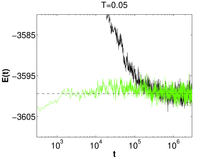
Figure 4: Plot demonstrating the difficulties in defining a clear time for whether and when equilibrium is reached. The dotted line represents the mean of the last half of the data points for the falling graph.

As an alternative, we can study the energy correlations of the system after it has reached equilibrium. We believe that the same timescales should be present both in the correlation function and in the final part of the relaxation process.

IV Analysis of system at equilibrium

IV.1 Energy correlations

The two-time energy correlation function is defined as

$$C(t,t+\tau)=\frac{1}{\sigma^{2}}\left<(E(t)-\bar{E})(E(t+\tau)-\bar{E})\right>$$ (8)

where $\bar{E}$ is the average energy and $\sigma$ is the standard deviation of the distribution of energies. The average should be over all realizations of the equilibrium dynamics. When studying the system at equilibrium, we use the fact that the system is stationary, and the correlation function will depend only on the time difference $\tau$. We can then use one simulated time evolution and average over starting times $t$ instead of over different realizations of the system, and write

$$C(\tau)=\frac{1}{\sigma^{2}}\left<(E(t)-\bar{E})(E(t+\tau)-\bar{E})\right>_{t}.$$ (9)

The average should include a large number of uncorrelated times, and this is only true if the period we average over is longer than the time scale of the correlations. Therefore the value of the correlation function for time differences $\tau>10^{6}$ should not be trusted for our time series of $10^{7}$ steps. Also, for long $\tau$ the correlation function shows a lot of noise, but interesting effects can be demonstrated at significantly shorter times than this. $C(\tau)$ at a number of temperatures is plotted in figure 5.

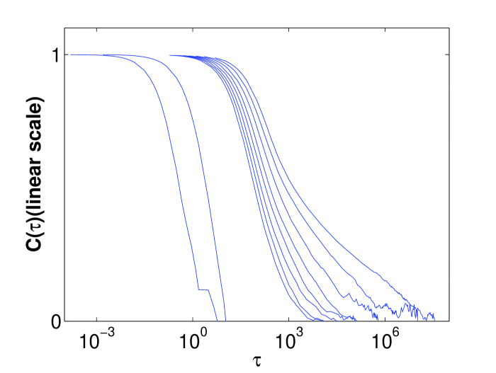
Figure 5: Plot of $C(\tau)$ at $T=\{0.03,0.04,0.05,0.06,0.07,0.08,0.09,0.1,1,10\}$

Kolton et al. Kolton made a similar analysis of the occupation correlation function for the three dimensional random site model. They proposed that one should plot the curves as function of the scaled variable $c_{T}t$ where $c_{T}$ is some temperature dependent relaxation rate. Based on a previous studyGrempel they assumed an activated law $c_{T}=e^{-T_{0}/T}$. We wanted to avoid this assumption, and instead extract the relevant rate from our numerical data using the following reasoning.

We try to model the evolution of the system as a random walk in energy. The probabilities of increasing or decreasing the energy at a particular step of the random walk is given by a combination of the transition rates given in Eq. (4), and the density of states. It can be shown that this is equivalent to the problem of a random walk in a harmonic potential. The details of the derivation are given in appendix B, the main results are that we expect the correlation function to decay exponentially, $C(\tau)=e^{-c_{T}\tau}$, with

$$c_{T}=\frac{\delta_{T}^{2}}{2\sigma_{T}^{2}\tau_{T}},$$ (10)

where $\delta_{T}$ is the mean of the absolute value of the energy change per electron jump at temperature $T$, $\sigma_{T}$ is the standard deviation of the distribution of the system energy at the same temperature, while $\tau_{T}$ is the average time per step. All these parameters are accessible from our simulations. Plots of the relevant $\sigma_{T}$, $\delta_{T}$, $\tau_{T}$ and $c_{T}$ are given in figure 6.

For the $\delta_{T}$, we see that it simply rises as $\delta_{T}=2T$, until the temperature becomes comparable with the spread of the single particle energies. $\sigma_{T}$, $\tau_{T}$ and $c_{T}$ all give fairly straight lines in the log-log plots, but we do not have sufficient data to conclude what functional dependency they follow. However, the previous suggestion of an activated law for $c_{T}$ does not seem to fit our data.

The interpretation of $c_{T}$ is also clear. Since the variance of a random walk grows linearly in time, $1/c_{T}$ is the time needed for the random walk to spread over a range equal to the equilibrium standard deviation, $\sigma_{T}$. In other words, it is the time at which the random walk starts to feel the effect of the constraining potential. While $c_{T}$ includes the size-dependent quantities $\sigma_{T}$ and $\tau_{T}$, it can be assumed that $c_{T}$ itself is size independent, as $\tau_{T}\propto N^{-1}$ while $\sigma\propto N^{1/2}$.

a)	b)
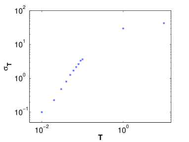
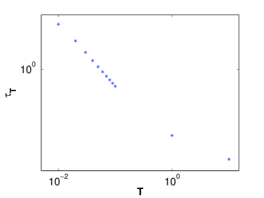
c)	d)

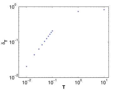
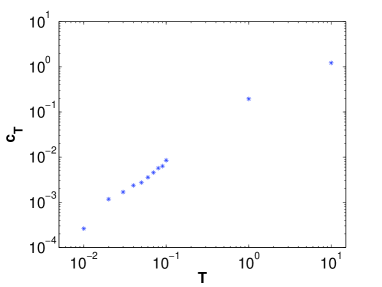
Figure 6: a) $\sigma_{T}$, width of the energy distribution b) $\tau_{T}$, average time per step c) $\delta_{T}$, mean of $|\Delta E_{i\rightarrow j}|$ d) $c_{T}=\frac{\delta_{T}^{2}}{2\sigma_{T}^{2}\tau_{T}}$

Fig. 7a shows the scaled correlation functions $C(c_{T}\tau)$, and as can be seen this gives an excellent collapse for the initial stage of the relaxation, but very poor for longer $\tau$.

a)	b)

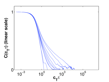
Figure 7: Attempts at collapsing the correlation functions. T={0.03,0.04,0.05,0.06,0.07,0.08,0.09,0.1,1,10} a) Scaling by $1/(2c_{T})$. High temperatures correspond to steep slopes b) $C(n)$, where $n$ is the number of steps, regardless of time spent. $T=\{1,10\}$ lie far away from the others.

Inspired by the apparent success of Kolton et al. Kolton in collapsing the curves, we made several attempts with other rescaling factors. The most successful was using $\tau_{T}$ as scaling factor, simply plotting the correlation as function of number of steps performed, as shown in Fig. 7b. We see that we get a picture resembling the collapse demonstrated by Kolton et al. for the random position model. But the deviations from a collapse are systematic, and by closer inspection of the inset of Kolton’s Fig. 2. we get the suspicion that their choice of zoom hides the fact that they have no true collapse either, as the difference between the curves in their scaled plot is an order of magnitude in time near both $C=1$ and $C=0$.

If we instead use the assumption of the exponential decay and plot $\ln(C(\tau))$ versus time, we expect to see straight lines. Figure 8 shows that this does indeed come close to the truth for $T=1,10$, but for the lower temperatures the lines are far from straight. Only at short times one might think that there can be some exponential decay. This can to some extent be further justified by plotting the scaled graphs $\ln(C(c_{T}\tau))$ (Fig. 8b). We see that the high temperature (T=1,10) graphs are close to straight lines whereas at lower temperature the graphs show a decay slowing with time, as longer and longer time scales come into play. At short times they approach the straight lines defined by the high temperature graphs, indicating short time exponential behavior, with the predicted $c_{T}$.

a)	b)

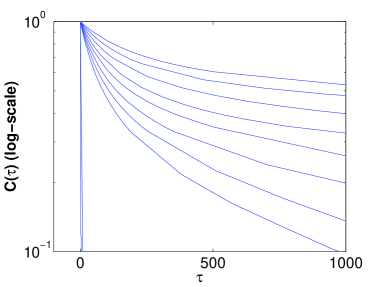
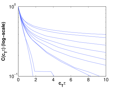
Figure 8: a) $C(\tau)$ b)$C(c_{T}\tau)$, $T=\{0.03-0.1,1,10\}$, we see signs of collapse at very short times, but only the highest temperatures give close to straight lines.

In disordered systems, it has previously been observedJund ; Ogielski that correlation functions can be well fitted by a stretched exponential function $C(\tau)=Ae^{-(\tau/\tau_{0})^{\gamma}}$. If that is true,

$$\ln{\frac{-\tau}{\ln(C(\tau))}}=\ln\frac{-\tau}{\ln A-(\tau/\tau_{0})^{\gamma}}\approx(1-\gamma)\ln\tau+\ln\tau_{0}^{\gamma},$$ (11)

for $\tau\gg\ln(A)$, and plotting $\ln\tau$ vs $\ln(-\tau/\ln C(\tau))$ we should get a straight line for large $\tau$. For a pure exponential, the line is horizontal, as $\gamma=1$ and $1-\gamma=0$. As the correlation function reaches the regime where only noise is left, $C(\tau)$ approaches a constant, $\gamma=0$ and $1-\gamma=1$ giving a line with slope $1$. As shown in Fig. 9, at short times we get a horizontal line for all temperatures, corresponding to the exponential decay that we have seen above. At low temperatures this crosses over to a straight line with some slope. We get straight lines for at least two orders of magnitude for the temperatures $T={0.03-0.1}$ before the correlation function drops below the noise level in our data and the graphs end in a noise dominated line of slope 1. At $T={1,10}$ we find straight horizontal lines that cross directly into the noise within our precision, without any intermediate region of stretched exponential behavior.

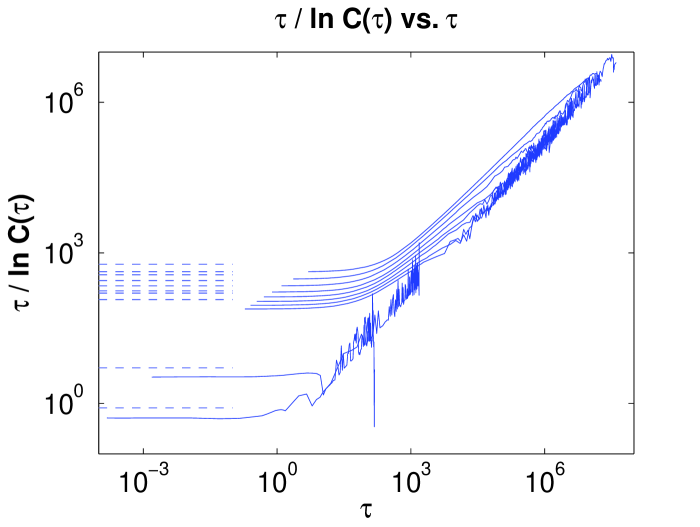
Figure 9: T={0.03,0.04,0.05,0.06,0.07,0.08,0.09,0.1,1,10} Horizontal lines indicate exponential behavior, slope of 1 indicates noise, while straight lines at other slopes indicate stretched exponential behavior. The dotted lines indicate $1/c_{T}$, as calculated using Eq. (10).

From the lines in Fig. 9 we can extract three values: the slope gives us $1-\gamma$, the offset at large $\tau$ allows us to determine $\tau_{0}$, and the initial level at which the behavior is exponential again gives us $c_{T}$. The fact that these initial levels are consistently slightly below our estimates for $c_{T}$ reflect the fact that locally, the width of the energy distribution is slightly smaller than for the full simulation time. Plots of $\gamma$ and $\tau_{0}$ vs temperature are given in Fig. 10.

a)	b)

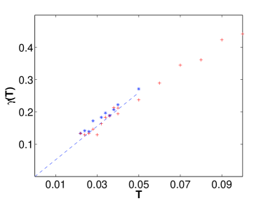
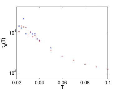
Figure 10: a) $\gamma(T)$ b) $\tau_{0}(T)$ The dashed line indicates a possible extrapolation towards $T=0$. The difference between the symbols denotes use of different cut-off limits when calculating jump rates, as discussed in appendix A. (*) denotes a limiting value $\Gamma_{min}=10^{-10}\Gamma_{tot}$, (+) denotes $\Gamma_{min}=10^{-7}\Gamma_{tot}$. For $\tau_{0}$ this makes no significant difference, but for $\gamma(T)$ we see that the more accurate simulation gives a slightly higher value of $\gamma(T)$. This is the only graph where the choice of limiting rate is noticeable, confirming that our algorithm is sufficiently accurate.

We see that as temperature goes down, $\tau_{0}(T)$ increases faster than exponential, and $\gamma(T)$ decreases almost linearly for small $T$, in both cases with the exception of $T=0.022,0.024$. We have also observed that the uncertainty, determined from the scattering of the points, increases for lower temperatures, as the time before all correlations are lost approaches the length of our time series. For the lowest two data points, we assume that our data are insufficient to give correct estimates for the standard deviation, $\sigma_{T}$, and mean, $\bar{E}$. Especially, if we look at too short time, we expect to measure a too small $\sigma_{T}$, so the correlation functions will therefore systematically underestimate the correlation. This will again give too high values for $\gamma(T)$ and too low for $\tau_{0}(T)$.

Again following OgielskiOgielski we can also define a weighted time

$$\tau_{\gamma}=\frac{\int\tau C(\tau)d\tau}{\int C(\tau)d\tau}$$ (12)

which can be seen as a weighted average time scale for processes in the equilibrium. Plotting $\tau_{\gamma}(T)$, obtained by numerical integration, we see that it increases dramatically as $T$ decreases (Fig. 11). If we assume $C(\tau)=e^{-(\tau/\tau_{0})^{\gamma}}$ we can find a relation between $\tau_{\gamma}$, $\tau_{0}$, and $\gamma$:

$$\tau_{\gamma}=\frac{\int\tau C(\tau)d\tau}{\int C(\tau)d\tau}=\tau_{0}\frac{\Gamma(2/\gamma)}{\Gamma(1/\gamma)}$$ (13)

where $\Gamma$ denotes the $\Gamma$-function. This value is also plotted in Fig. 11. The errors in these plots are huge, especially at low temperatures, due to the following two effects. First, due to the extreme sensitivity of the analytical estimate Eq.(13) to the value of $\gamma$, any uncertainty in $\gamma$ translates into a much larger uncertainty in $\tau_{\gamma}$. Second, the long and noisy tail of $C(\tau)$ makes numerical integration difficult. In cases where $C(\tau)$ does not reach zero within our simulation time, numerical integration becomes impossible. The correlation $C(t_{1},t_{1}+\tau)$, as defined in Eq. (8), can not be considered independent of $C(t_{2},t_{2}+\tau)$ unless $t_{2}-t_{1}>\tau$. When using Eq. (9), the number of independent time intervals we average over can be estimated as the total simulation time divided by $\tau$. Therefore, the noise increases with $\tau$. To improve this, we have averaged over from 3 to 10 independent time series at the lowest temperatures. Still, both estimates for $\tau_{\gamma}$ show an increase that is at least exponential as $T$ decreases. This again justifies disregarding $T=\{0.024,0.026\}$ as our simulation time does not come near these time scales.

If we assume $\gamma(T)\propto T$, which does not seem impossible for small $T$, the gamma functions in Eq.13 can be estimated using Stirling’s formula to give an estimate for $\tau_{\gamma}$ as

$$\tau_{\gamma}\propto\tau_{0}(T)\frac{1}{T}^{\frac{1}{T}}e^{-\frac{1}{T}}2^{\frac{1}{T}}$$ (14)

There is no way we can differentiate between this kind of behavior and a divergence at a specific temperature within our data. Any divergence in $\tau_{\gamma}$ would have to come from either $\gamma$ going to zero, which appears to happen at $T=0$ if we extrapolate linearly, or from a divergence in $\tau_{0}$, which we have not been able to identify.

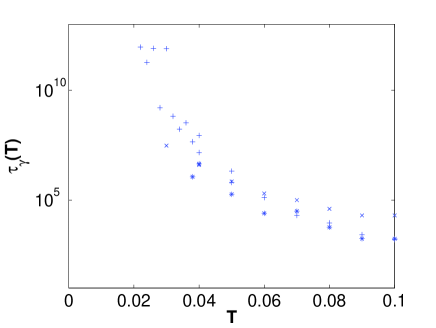
Figure 11: $\tau_{\gamma}(T)$ from numerical integration (*) $\tau_{\gamma}(T)$ from equation (13) (+) and the visual estimate of the relaxation time (x).

IV.2 Global density of states

Originally, the dynamics of the Coulomb Glass were understood mainly from the single electron jump picture, giving rise to the theory of the Coulomb Gap,EfrosShklovskii which is a gap in the single electron density of states. But in order to say something about behavior at higher temperatures, we should also know something about the global density of states far away from the ground state, especially as our results show that all our visited states are likely to be far from the ground state.

The probability $P(E)$ of the system being at an energy $E$ is assumed to be simply the product of the probability of a given state being occupied times the density of states at this energy, $g(E)$, giving

$$P(E)=\frac{1}{Z}g(E)f(E,T),\qquad Z=\sum_{E^{\prime}}f(E^{\prime},T)g(E^{\prime})$$ (15)

where $f(E,T)=e^{-\beta E}$, $\beta=1/T$, as we have chosen to measure temperature in the same units as energy. If we assume that the simulation time suffices for the distribution of energies we observe to be representative for the behavior at infinite times, we can use the observed $P(E)$ to estimate $g(E)$. If we furthermore assume the system to be ergodic, $g(E)$ will be the actual density of states of the full system. If not, $g(E)$ is just the density of states accessible from the set of states we have visited, while the global density of states is a sum of different $g(E)$-s. We have tried relaxing the system from different electron configurations, and seen no trace of variation in the equilibrium distribution. While this does not constitute any proof, we can at least conclude that the system is either ergodic, or that $g(E)$ is the same for multiple separate sets of configurations.

At low temperatures, where we are not able to reach equilibrium we can still consider one step (as defined in Fig. 2b) on a descending graph. Then we get the density of states for the set of states accessible by likely transitions, a set sometimes referred to as a valley in configuration space. This is the case in the plots for $T=0.01$ in Figs. 12 and 13.

Fig. 12 shows $P(E)$ calculated from the number of times a state with energy $E$ is visited, weighted by the time spent in that configuration.

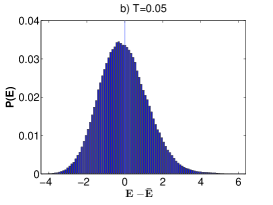
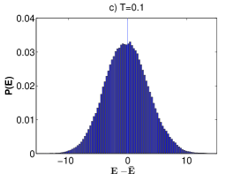
Figure 12: Histograms of $P(E)$ for T={0.01,0.05,0.1}. The histogram is for the last $10^{6}$ jumps of a run of $10^{7}$ jumps, except for $T=0.01$, where only $8\cdot 10^{5}$ where included to stay within one step. It is seen that at high temperature the distribution is symmetric, whereas the lack of symmetry for $T=0.01$ is clear. The vertical lines indicate $\bar{E}$, the mean of the equilibrium distribution.

Solving Eq. (15) for $g(E)$ we write

$$g(E)=P(E)f(E,T)^{-1}\sum_{E^{\prime}}f(E^{\prime},T)g(E^{\prime})$$ (16)

Note that $g(E)$ is written as a vector of values for discrete energies $E$. This is due to our discretization of $P(E)$ in the form of histogram boxes. Defining the matrix $M_{EE^{\prime}}=P(E)f(E,T)\sum_{E^{\prime}}f(E^{\prime},T)$ we can write this as

$$g(E)=\sum_{E^{\prime}}M_{EE^{\prime}}g(E^{\prime})$$ (17)

Thus $g(E)$ must be an eigenvector of the matrix $M_{EE^{\prime}}$, with eigenvalue 1. In this way we can find $g(E)$ except for a constant prefactor $g_{0}$.

The calculated $g(E)/g_{0}$ for our equilibrium distributions are shown in Fig. 13.

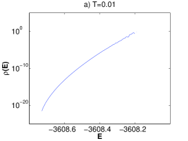
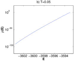
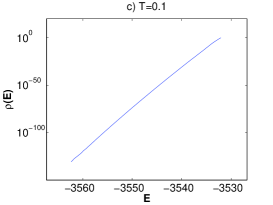
Figure 13: Estimated $g(E)/g(E_{T})$ from the distribution at $T=\{0.01,0.05,0.1\}$. For $T=0.01$ we clearly see that $\rho=\ln(g(E))$ has a strong curvature, for $T=\{0.05,0.1\}$ the curvature is less pronounced, but still present.

Note that the plot shows $\ln(g(E)/g(E_{T}))$, where $E_{T}$ is the highest energy obtained at equilibrium for this temperature. Within the energy region covered by each run, the density of states approaches a straight line, for more than hundred orders of magnitude in $g$ in the case of $T=0.1$.

Based on the obtained results, we choose to write $g(E)=g_{0}e^{\rho(E)}$, where $\rho(E)$ is well defined for energies well above the ground state, $E_{0}$.

$$P(E)=\frac{e^{\rho(E)-\beta E}}{Z}$$ (18)

has a maximum when

$$\frac{dP(E)}{dE}=\frac{1}{Z}\left(\frac{d\rho(E)}{dE}-\beta\right)e^{\rho(E)-\beta E}$$ (19)

equals zero. We can thus expect the maximum of the distribution, $E_{m}$, to be in an area where the rise in DOS is comparable to the inverse temperature, $\rho^{\prime}(E_{m})=\beta$. Lower temperature requires a steep rise in DOS to reach equilibrium, whereas at higher temperature equilibration will occur with slower increases in DOS.

To find the width of the distribution we write $E=E_{m}+\Delta E$, where $E_{m}$ is the previously obtained energy corresponding to the maximum of the distribution, for which we know that $\rho^{\prime}(E_{m})=\beta$. An expansion of $P(E)$ to the second order in $\Delta E$ then gives:

$$P(E)=\frac{1}{Z}e^{\rho(E)-\beta E}=\frac{1}{Z}e^{\rho(E_{m})+\rho^{\prime}(E_{m})\Delta E+\rho^{\prime\prime}(E_{m})\Delta E^{2}/2-\beta(E_{m}+\Delta E)}.$$ (20)

Separating the $E_{m}$ dependence from the $\Delta E$ dependence this gives

$$P(E)=\frac{e^{\rho(E_{m})-\beta E_{m}}}{Z}e^{\rho^{\prime\prime}(E_{m})\Delta E^{2}/2},$$ (21)

which shows that the standard deviation of the distribution is $\sigma=1/\sqrt{|\rho^{\prime\prime}(E_{m})|}$. In this way we can readily find both $\rho^{\prime}(E)$ and $\rho^{\prime\prime}(E)$ at as many energies as the number of temperatures at which we run relaxations.

The most immediate use of this information is probably for algorithms requiring the mapping of all states accessible for the system.Pollak Estimating $P(E)$ gives an upper temperature limit for which one can hope to map all states, for a given system size.

V Discussion

V.1 Validity of the random walk model

We see that for high temperatures, $T=\{1,10\}$ the model of the random walker seems to be a good description of the observed dynamics. Regarding both the density of states and the short time correlations, the same is true for the lowest temperatures still reaching an equilibrium. But for longer times, the correlations persist much longer than our estimates for $c_{T}$ should indicate.

Some general understanding that has been suggestedCampbell is that at high temperatures the network of thermally allowed transitions is sufficiently dense in the space of configurations that the number of possible jumps is a function of the density of states (DOS) only. The system performs a random walk on this network, which when projected on the energy gives the random walk in energy that we have considered above, and exponential decay of the correlation function. Below some temperature $T_{c}$ the network of allowed transitions becomes diluted and has some fractal structure. A random walk on this fractal leads to anomalous diffusion $\left<r^{2}\right>\propto t^{\gamma}$, which is believed to correspond to a stretched exponential $e^{-(\tau/\tau_{0})^{\gamma}}$ for the correlation function of any confined quantity like our energy, both with the same exponent $\gamma$ (As far as we are aware, this has only been numerically confirmed for hypercubesCampbell and hyperspheresJund and not rigorously established). Thus, we expect that as temperature increases, $\gamma$ should also increase, and approach 1 at $T_{c}$. We see from Fig. 10 that this seems to be the case, but our data are not sufficient to determine $T_{c}$. In this temperature regime a standard Metropolis algorithm would be more suitable than our low temperature algorithm. It has also been suggestedCampbell that because the configuration space has a large dimension, $\gamma$ should approach the mean field value of percolation, $\frac{1}{3}$, at the glass transition. This was indeed the case in the work of Ogielski,Ogielski but is clearly not the case in our simulations. $\gamma$ reaches a value of approximately 0.15 at $T=0.03$, but can possibly be estimated to even lower values with better data sets.

V.2 Possible model system

To give a picture of what kind of model could adequately describe this picture, we start from a landscape of local minima, defined by the fact that there exist no single electron transitions taking the system down in energy. We have previously shown that there exist a huge number of such minima.Glatz

From each local minimum, we can find all states that can be reached by one single electron jump, by definition taking the system up in energy. From each of these states, we can again add states accessible by another jump, and so on, but keeping only those that increase the energy. In this way we create a tree growing up from each local minimum. It is easy to imagine these single trees having an initial exponential growth in the density of states. As the states of one tree become identified with states of other trees, the exponential growth slows because the number of identified states increases drastically. We have attempted to illustrate this in Fig. 14

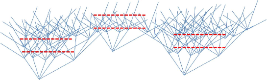
Figure 14: Simplified picture of the configuration space. The dotted lines indicate regions with similar increase in density of states, but at different energies, due to different starting points.

The branch thickness is described by the wave function overlap of the two states involved in that specific transition, and is temperature independent. In addition, at each temperature, there is a likelihood of passing up the branch different from that of passing down the branch, given by energy difference, temperature, and branch thickness. If we define a minimum jump probability given by the time scale of our experiment, we can cut away all branches with lower probabilities than the limiting value, like in a random resistor network. As temperature goes down, more and more branches will be cut or made one-way streets for the purpose of system development. The resulting network will resemble a fractal network with a temperature dependent dimension.

A random walker on such a network will show dynamics on many competing time scales. First, within the branches of one ’tree’, there is the time scale to make single jumps, corresponding to our $\tau_{T}$. Then comes the time scale for getting from the bottom of a ’tree’ to the top, or opposite, which is approximately $1/c_{T}$. Then there is the probability of jumping from one ’tree’ to another, from one cluster of ’trees’ to another, between clusters of clusters and so on. The average energy of the clusters can vary, giving correlations over long time scales as we slowly climb from one cluster to the next. This process is described by the slow decay of the correlation function $C(\tau)$. When temperature is lowered, the probability of reaching the top branches will be reduced, and there will be fewer or less likely connections between the different ’trees’ and clusters. The probability of jumping to lower clusters will decrease, but that of jumping to higher energy clusters will decrease even more. Such a random walk should behave much like our simulation.

While we believe that such a model will lead to the observed behavior, we have no independent verification that this model actually corresponds to our system.

V.3 Temperature and time scales

As mentioned in the introduction, one of our objectives in undertaking this project was to identify a glass transition temperature and a dynamic phase diagram for the lattice model. While we have not been able to identify a transition temperature, or determine whether such a finite temperature exists, we have identified timescales where the system will equilibrate as function of temperature. If we wish to study the time evolution of some quantity, we have to average over time intervals shorter than this equilibration time.

Tsigankov et al.Tsigankov studied the lattice model that we have used and compared it with the random site model. They were interested in the long time relaxation of the conductance observed in experiments,Ovadyahu but since the direct simulation of this process would take too long time, they calculated the conductance and the shape of the Coulomb gap for various initial states, arguing that if one is to observe slow relaxation one would need to find metastable states with sufficient spread in conductance. Their simulations were performed at $T=0.04$ as this was the lowest temperature they were able to use for their algorithm to be efficient. They observed that the variation in the conductance for the lattice model was too small to explain the observed change in the conductance during slow relaxation and concluded that the lattice model can not be used to explain the experiments. With our optimized algorithm we are able to go below this and we have shown that we are able to reach equilibrium for temperatures at least down to $T=0.03$, possibly as low as $T=0.02$. Therefore we believe that the results of Tsigankov et al.Tsigankov are probably a result of using a temperature where the system equilibrates, and that their conclusion could be different if they could repeat their simulation at lower temperature, below some glass transition temperature $T_{g}$, or at least in a region where $\tau_{\gamma}$ is greater than the simulation time span. It should be noted that Tsigankov et. al. use localization length $a_{l}=1$ rather than our $a_{l}=2/3$. We believe that increasing $a_{l}$ allows more connections between the different regions of the configuration space, in the same way as an increase of temperature. Thus, Tsigankov’s temperature $T=0.04$ would be equivalent to a higher temperature in our simulations. This argument agrees well with the relation between temperature and localization length in the expression for conductance, which is a function of the product $a_{l}T$.EfrosShklovskii ; Tsigankov2

VI Conclusions

Based on the above analysis, we have reached the following conclusions:

• For temperatures down to a limiting $T_{min}\approx 0.02$ we have demonstrated that the system equilibrates within our simulation time. This equilibration occurs at a total system energy for which the total number of accessible states is so high that a full mapping of the states is only possible for very small systems.

• At temperatures close to, but above $T_{min}$ we observe energy correlations following a stretched exponential law. The exponent of this stretched exponential, $\gamma$, decreases with temperature, seemingly with a linear dependence for low temperatures. At temperatures $T\gtrsim 1$, $\gamma$ approaches unity, but determining the exact behavior requires further study.

• $\tau_{\gamma}$, the average relaxation time weighted by the correlation function, increases rapidly with decreasing temperature. It seems to roughly follow the time needed to establish equilibrium.

• The rapid increase of $\tau_{\gamma}$ with decreasing temperature, means that the low temperature limit for when equilibrium can be established is only weakly dependent on the total simulation time. From our data we cannot conclude whether $\tau_{\gamma}$ actually diverges at any finite temperature, or whether it can be used to define a glass transition.

• The observed behavior is compatible with a model of the system as a random walk on a fractal configuration space.

• There exists a temperature range for which the lattice model with single electron hops only, can probably be used to study slow dynamics.

It is important to stress that we have shown the time scales of the single jump dynamics only. As the correlation times become longer, processes that are unlikely when looking at single changes of state may still be important for the long term dynamics of the system. We have only shown that single jumps can give long time scales, not that these time scales will actually be present in the model if other dynamics are also allowed. Specifically, multi-electron jumps are likely to hasten the transitions between state clusters at low temperatures, giving shorter correlation times and larger values for $\gamma(T)$.

Appendix A Details of relaxation algorithm and parameter choices

We use Monte Carlo simulation, first calculating the probabilities of all those jumps that are likely to occur from a given configuration, and choosing one of them to actually happen. The physical time spent on one such step is calculated as the inverse of the sum of all the rates for individual jumps. The limitation of the basic model is therefore that it allows single particle jumps only.

The rate for a single jump is given in Eq. (4). This expression is only strictly valid when there is a constant barrier height. In our system this is not the case, as the charge distribution gives valleys and peaks in the barrier over the volume the electron wave function covers. A proper treatment would have to include an integral over all possible paths. We still follow the tradition in the field and use the expression above, as the exact alternative would be impossible to implement.

Calculating all possible jumps is still a very time-consuming process. Following Ortuño et al. Ortuno we therefore limit ourselves to calculating those jumps that are probable to occur. We see that eq (4) decays exponentially both with distance and energy difference. Therefore, a very few rates will be big, while the majority of rates will be neglectably small. It is therefore possible to write

$$\Gamma_{tot}=\sum_{i,j}\Gamma_{i\rightarrow j}=\sum_{prob}\Gamma_{i\rightarrow j}+\sum_{improb}\Gamma_{i\rightarrow j}\approx\sum_{prob}\Gamma_{i\rightarrow j}$$ (22)

assuming the latter sum, over improbable jumps, to be negligibly small. The first sum, the probable jumps, can be shown to include only a relatively small number of jumps, depending on the configuration. A similar thought is used in the algorithm presented by Matulewski et. al.Matulewski2 , even though their implementation is more static than ours.

We define a limiting rate $\Gamma_{min}$ so that only jumps where $\Gamma_{i\rightarrow j}>\Gamma_{min}$ are included in the first sum.

$$\Gamma_{min}=\Gamma_{0}e^{-M}$$ (23)

where $M$ is the maximal allowable exponent to give rates higher than $\Gamma_{min}$. For the simulations presented we have chosen to set $\Gamma_{min}$ to $10^{-7}\Gamma_{tot}$ for the higher temperatures, where our algorithm is slow, and $10^{-10}\Gamma_{tot}$ for low temperatures. Since $\Gamma_{tot}$ is only known after all the rates are calculated, we use the $\Gamma_{tot}$ from the previous step in calculating $\Gamma_{min}$. The validity of our approach can be tested by varying the ratio $\Gamma_{min}/\Gamma_{tot}$, and see whether it influences the dynamics, as shown in Fig. 9. A simple estimate on the error made can be obtained as illustrated in Fig. 15. Here we have calculated the rates of all jumps, and sorted them by magnitude. We define $\Gamma_{n}$ as the $n$’th largest rate. Plotting the individual and cumulative probabilities together, we can immediately read off the error we make if we cut off all rates with a value less than a certain fraction of the total rate. Our cut-off at $10^{-7}\Gamma_{tot}$ means that in this randomly chosen instance at $T=0.02$, we would need to include 1200 jumps, and make an error in the total rate of less than $2\cdot 10^{-5}\Gamma_{tot}$. This means that approximately 10 jumps are erroneously cut off in $10^{6}$ steps.

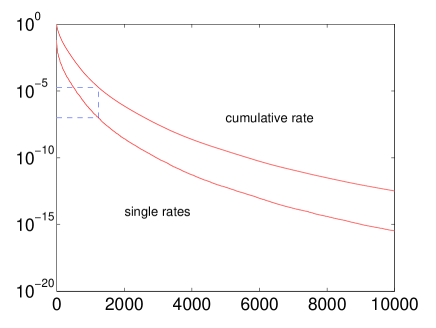
Figure 15: $\Gamma_{n}/\Gamma_{tot}$ and $(\sum_{n^{\prime}<n}\Gamma_{n^{\prime}})/\Gamma_{tot}$ vs $n$. Dotted lines indicate the cut-off limit and corresponding error.

The selection of which rates to calculate is optimized using the $M$ defined above. We wish to cut off improbable rates, that is rates where the increase in energy is much larger than temperature, or where distances are very long. From the expression given for the tunneling rate in Eq. 4, using the expression for phonon absorption, we can take the $1$ in the denominator to be small, which simplifies our requirement for the limiting tunneling rate to the expression

$$|\Delta E_{i\rightarrow j}|/T+2r_{i,j}/a_{l}<M,$$ (24)

disregarding the preexponential factor which further reduces the rate for low temperatures. We also know that the energy difference is given as

$$\Delta E_{i\rightarrow j}=\epsilon_{j}-\epsilon_{i}-1/r_{i,j}$$ (25)

and the minimum value for $\epsilon_{j}$, $\epsilon_{j,min}$ can easily be found from the list of single particle energies. So

$$\epsilon_{j,min}-\epsilon_{i}-\frac{1}{r_{i,j}}\leq\epsilon_{j}-\epsilon_{i}-\frac{1}{r_{i,j}}=\Delta E_{i\rightarrow j}\leq T\left(M-\frac{2r_{i,j}}{a_{l}}\right)$$ (26)

Thus for each $\epsilon_{i}$ there is a given maximal radius that can potentially give probable jumps. Conversely, for each radius, there is a lowest allowable $\epsilon_{i}(r)$. If $\epsilon_{i}(r)$ is below this limit, there is no point in looking for empty sites further away than the given radius.

In the initial stages, many jumps are very likely, so $\Gamma_{tot}$ and therefore also $\Gamma_{min}$ is very large. This gives a small maximal radius for all sites, regardless of $\epsilon_{i}$. While long jumps could possibly happen, it is much more likely that a short jump happens first.

As soon as the Coulomb Gap has formed, there will be very few sites where the $\epsilon_{i}$ is sufficiently high to allow long jumps to be probable. Only for these occupied sites do we have to check many possible destinations, and many sites will have no likely jumps at all. Thus for both situations, with and without gap, the number of calculated rates scale roughly as $N$ rather than $N^{2}$.

As observed by Ortuño et al.,Ortuno there is often a limited number of jumps that are repeated a very large number of times. Ortuño et al.Ortuno solve this by calculating the rate to escape from an ensemble of configurations. We have used a faster and easier approach, where we simply save the state and jump rates for each configuration, until a jump occurs that is unlikely to be reversed. Every time a state is revisited, we only have to switch some pointers. The disadvantage of this approach is that we record a huge number of jumps that are simply repetitions, but it does not cost us much computation time. The advantage is that we record the time spent at all configurations explicitly, making it possible to easily extract information on thermal properties, noise etc. Also, our algorithm is faster in those cases where a configuration is not revisited. For very low temperatures, $T\lesssim 0.001$, the number of repeated jumps becomes impracticable large. In this case Ortuño’s algorithm will probably work better than ours.

The algorithm used is optimized to work best for temperatures where the Coulomb Gap has formed properly, so both the energy and the distance terms give fast convergence for the sums. Thus the initial phase of relaxation will be computationally slower per step. Also, higher temperatures give a slower convergence in the energy term, and thus longer processing times. At some temperature, the optimized Metropolis algorithm of Ref. Tsigankov, becomes significantly more efficient. Preliminary tests indicate that this happens around $T=0.05$.

In order to have a constant ground state and density of states, all simulations presented in this article are based on the same realization of disorder of the lattice. Some preliminary results for conductance simulations indicate that a system of $100^{2}$ sites may still be too small to avoid size effects for diffusive processes. On the other hand, we expect a requirement for longer time series for bigger systems, and the combined increase in computational effort of the bigger system and longer time makes it impractical to simulate. For most of the simulations we have been limited to using desktop computers, reducing our capacity for obtaining optimal statistics, but we still consider the results to be sufficient to give trustworthy conclusions.

The localization length is somewhat arbitrarily set to $2/3a$, where $a$ is the lattice constant. If we use localization lengths larger than $a$, mixing of the states would give significant changes in the wave functions. If we use a very short localization length, jumps longer than to the nearest neighbor will become highly improbable at all but the very lowest temperatures, enhancing the importance of the quadratic lattice. $a_{l}=2/3a$ gives a significant number of jumps at distances up to three sites away, but rarely longer, for the most relevant temperature range.

Appendix B Theory of a Random Walker in a potential

Let $u(x,t)$ be the probability of finding the random walker with position $x$ at time $t$. Let it take steps of length $\delta$ either increasing or decreasing its energy and let $\tau$ be the time of each step. Then the master equation for $u(x,t)$ is

$$u(x,t+\tau)=p(x-\delta)u(x-\delta,t)+q(x+\delta)u(x+\delta,t)$$

where $p(x)$ is the probability of making a step in the direction of increasing $x$ when the walker is at energy $x$ and $q(x)$ the probability of making a decreasing step. Expanding to first order in $\tau$ and second order in $\delta$ we get

$$\frac{\partial u}{\partial t}=(q-p)\frac{\delta}{\tau}\frac{\partial u}{\partial x}+\frac{\partial}{\partial x}(q-p)\frac{\delta}{\tau}u+\frac{\delta^{2}}{2\tau}\frac{\partial^{2}u}{\partial x^{2}}$$ (27)

where we have used that

$$\frac{\partial}{\partial x}(p+q)=\frac{\partial^{2}}{\partial x^{2}}(p+q)=0.$$ (28)

We need to find expressions for $p(x)$ and $q(x)$. The requirement of microscopic balance (and one can check that our Monte Carlo algorithm satisfies this) is

$$p(x)P(x)=q(x+\delta)P(x+\delta)$$ (29)

where $P(x)$ is the probability of finding the system at position $x$. As discussed in Sec. IV.2 this can be written $P(x)=Ae^{\frac{\rho^{\prime\prime}}{2}x^{2}}$ close to the equilibrium position. We will assume that the probability $q(x)$ changes slowly on the scale of a single step $\delta$. This allows us to replace $q(x+\delta)$ with $q(x)$ on the right hand side of Eq. (29) and using $p(x)+q(x)=1$ we get

$$p(x)=\frac{e^{\rho^{\prime\prime}\delta x}}{1+e^{\rho^{\prime\prime}\delta x}},\quad q(x)=\frac{1}{1+e^{\rho^{\prime\prime}\delta x}},$$

where we have omitted the $\delta^{2}$-term in the exponent. Expanding to lowest order in $\delta$ we find

$$q(x)-p(x)=-\frac{1}{2}\rho^{\prime\prime}\delta x$$

Inserting this in Eq. (27) we get

$$\frac{\partial u(x,t)}{\partial t}=D\frac{\partial^{2}u(x,t)}{\partial x^{2}}+c\frac{\partial}{\partial x}(xu(x,T))$$ (30)

where $D=\frac{\delta^{2}}{2\tau}$ and $c=\frac{\delta^{2}}{2\sigma^{2}\tau}$. Eq. (30) is the diffusion equation in the presence of a harmonic potential. This is identical to the problem of momentum distribution of a particle under Brownian motion, and an exact solution has been provided by ChandrasekarChandrasekar :

$$u(x,x_{0},t)=\frac{1}{\sqrt{2\pi}}\sqrt{\frac{c}{D(1-e^{-2ct})}}e^{-\frac{(x-x_{0}e^{-ct})^{2}c}{2D(1-e^{-2ct})}}.$$ (31)

where $x_{0}$ is the starting position. We see that this solution has the properties we expect, becoming a delta function for $t\rightarrow 0$, it always has a Gaussian shape, and as $t\rightarrow\infty$ we get standard deviation $\sigma=\sqrt{D/c}$ and mean $0$ as expected.

Looking at the expectation value of the position as function of time, we find

$$\left<x(t)\right>=x_{0}e^{-ct}.$$ (32)

Thus if we initiate the system at at position $x_{0}$, we expect it to relax exponentially towards the equilibrium value as $e^{-ct}$.

We can now define the probabilities $P(E_{0})$, the probability of starting at a given energy $E_{0}$, and $P(E,t|E_{0},0)$, the probability of being at $E$ at time $t$ given that the system was at $E_{0}$ at time $0$. From the two-time energy correlation function we can identify $P(E_{0})=u(t=\infty)$, while $P(E,t|E_{0},0)=u(E,E_{0},t)$, giving

$$C(t)=\frac{1}{\sigma^{2}}\int\int dE_{0}dE\,E_{0}Eu(\infty)u(E,E_{0},t)$$ (33)

$$=\frac{1}{2\pi\sigma^{2}}\frac{c}{D}\frac{1}{\sqrt{1-e^{-2ct}}}\int\int dE_{0}dEE_{0}Ee^{-\left[\frac{cE_{0}^{2}}{2D}+\frac{(E-E_{0}e^{-ct})^{2}c}{(1-e^{-2ct})2D}\right]}$$ (34)

which integrates out surprisingly beautifully to give simply

$$C(t)=e^{-ct},\qquad c=\frac{\delta_{E}^{2}}{2\sigma^{2}\tau}.$$ (35)

We see that all information on the diffusion rate $D$ has been removed from the correlation function, only the relation between step length and the standard deviation remains.

Appendix C Statistics of steps at low temperatures

We made a simple analysis to see whether any information could be extracted from the distribution of the steps observed. We define a ’step’ by the setting of a new record low energy. We define $t_{w}$ to be the waiting time from one record energy to the next, while the energy difference between the two records is defined as the step size $\delta_{s}$. If multiple consecutive jumps take the system down in energy, only the state after the last one is accepted as a ’step’. This still gives some artificial small $\delta_{s}$ whenever it takes several steps before a local minimum is reached, so we can ignore those steps that correspond to very small $\delta_{s}$. In this region there is also a rounding error in the saved files, giving an artificial discretization of measured $\delta_{s}$.

There is also evidence of steps going up in energy. These will not be found by our algorithm, but for sufficiently low temperatures they do not seem to play an important role.

Plots of $t_{w}$ and $\delta_{s}$ as functions of time are given in Fig. 16. The data are for four different relaxations at $T=0.001$. We see that while there is a tendency that the step size $|\delta_{s}|$ decreases with time, the $t_{w}$ shows a much more pronounced behavior. The maximum waiting time increases close to linearly with $t$. Thus the slowing down of the relaxation seems to be due to longer waiting times than due to smaller records being set. We have not attempted any theoretical explanation of these results.

a)	b)

Figure 16: a) $t_{w}$ vs $t$ b)$\delta_{s}$ vs $t$, four separate runs (o,+,*,x) at $T=0.001$.

References

- (1) N. F. Mott, J. Non-Cryst. Solids 1, 1 (1968).
- (2) J. H. Davies, P. A. Lee and T. M. Rice, Phys. Rev. Letters, 49, 758 (1982).
-
(3)
B. I. Shklovskii and A. L. Efros, Electron Properties of Doped Semiconductors, Springer Series in Solid-State Sciences 45 (Springer, Berlin, 1984)
A. L. Efros and B. I. Shklovskii, J. Phys. C 8, 49 (1975). - (4) Z. Ovadyahu, Phys. Rev. B. 73, 214208 (2006).
- (5) S. Kar, A. K. Raychaudhuri, A. Ghosh, H. v. Löhneysen and G. Weiss, Phys. Rev. Letters91 216603 (2003).
- (6) T. Kurosawa and H. Sugimoto, Progr. Theor. Pys. Suppl. 57 217 (1975).
- (7) J. Matulewski, S. D. Baranovskii and P. Thomas, Physica status solidi. B. 245 3 pp. 481-484 (2008).
- (8) A. Díaz-Sánchez, A. Möbius, M. Ortuño, A. Neklioudov and M. Schreiber, Phys. Rev. B 62 8030 (2000)
- (9) A. M. Somoza, M. Ortuño, M. Pollak, Phys. Rev. B 73, 045123 (2006)
- (10) N. Metropolis, A. W. Rosenbluth, M. N. Rosenbluth, A. H. Teller, E. Teller, J. Chem. Phys. 21 1087 (1953)
- (11) D. N. Tsigankov, E. Pazy, B. D. Laikhtman, and A. L. Efros, Phys. Rev. B, 68 184205 (2003)
- (12) A. B. Kolton, D. R. Grempel, D. Domínguez, Phys. Rev. B 71 024206 (2005)
- (13) E. R. Grannan and C. C. Yu, Phys. Rev. Letters, 71 3335 (1993)
-
(14)
A. Möbius, P. Thomas, Phys. Rev. B 55 7460 (1997)
A. Möbius, P. Thomas, J. Talamantes and C. J. Adkins, Phil. Mag. B 81, 1105 (2001) - (15) M. Ortuño, M. Caravaca, A. M. Somoza, Phys. Stat. Sol. (c) 5, 3 647-679 (2008)
- (16) A. M. Somoza, M. Ortuño, M. Caravaca and M. Pollak, Phys. Rev. Letters 101 056601 (2008)
- (17) A. T. Ogielski, Phys. Rev. B, 32 7384 (1985)
- (18) A. Möbius, M. Richter and B. Drittler, Phys. Rev. B 45 11568 (1992)
- (19) A. Glatz, V. M. Vinokur, J. Bergli, M. Kirkengen, Y. M. Galperin, Journ. Stat. Mech. (2008) P06006
- (20) F. G. Pikus and A. L. Efros, Phys. Rev. Lett. 73, 3014 - 3017 (1994)
- (21) D. R. Grempel, Europhys. Letters, 66 6 845-860 (2004)
- (22) P. Jund, R. Jullien, I. Campbell, Phys. Rev. E 63, 036131 (2001)
-
(23)
I. A. Campbell, J. Phys. (France) Lett. 46, L1159 (1985)
I. A. Campbell, Phys. Rev. B 33 3587 (1986)
I. A. Campbell, J. M. Flesselles, R. Jullien and R. Botet, J. Phys. C 20, L47 (1987)
N. Lemke and I. A. Campbell, Physica A 230, 554 (1996) - (24) D. N. Tsigankov and A. L. Efros, Phys. Rev. Letters, 88 176602 (2002)
- (25) J. Matulewski, S. D. Baranovskii and P. Thomas, Phys. Stat. Sol. (c), Volume 5, Issue 3 (p 694-698) (2008)
- (26) S. Chandrasekar, Reviews of Modern Physics 15 1 (1943)