Discovery of molecular shells associated with supernova remnants. (II) Kesteven 75

Abstract

The young composite supernova remnant (SNR) Kesteven 75, with a pulsar wind nebula at its center, has an unusual morphology with a bright southern half-shell structure in multiwavelengths. The distance to Kes 75 has long been uncertain. Aiming to address these issues, we have made millimeter spectroscopic observations of the molecular gas toward the remnant. The $V_{\rm LSR}\sim$ 83–96 km s^-1 molecular clouds (MCs) are found to overlap a large north-western region of the remnant and are suggested to be located in front of the SNR along the line of sight. Also in the remnant area, the $V_{\rm LSR}$= 45–58 km s^-1 MC shows a blue-shifted broadening in the ¹²CO (J=1-0) line profile and a perturbed position-velocity structure near the edge of the remnant, with the intensity centroid sitting in the northern area of the remnant. In particular, a cavity surrounded by a molecular shell is unveiled in the intensity map in the broadened blue wing (45–51 km s^-1), and the southern molecular shell follows the bright partial SNR shell seen in X-rays, mid-infrared, and radio continuum. These observational features provide effective evidences for the association of Kes 75 with the adjacent 54 km s^-1 MC. This association leads to a determination of the kinematic distance at $\sim 10.6\,{\rm kpc}$ to the remnant, which agrees with a location at the far side of the Sagittarius arm. The morphological coincidence of the shell seen in multiwavelengths is consistent with a scenario in which the SNR shock hits a pre-existing dense shell. This dense molecular shell is suggested to likely represent the debris of the cooled, clumpy shell of the progenitor’s wind bubble proximately behind the 54 km s^-1 cloud. The discovery of the association with MC provides a possible explanation for the $\gamma$-ray excess of the remnant.

1. INTRODUCTION

Massive stars have often not moved far from their matrices in molecular clouds (MCs) by the time they explode as core-collapse supernovae because of their short lifetime, and therefore their remnants are often observed to be associated with MCs. The CO observations have demonstrated a good positional correlation between MC complexes and supernova remnants (SNRs) (Huang & Thaddeus 1986). About 20 SNRs are known to physically interact with ambient MCs with convincing evidences (e.g. Frail et al. 1996). The interaction of either the progenitors’ stellar winds or the SNR shocks with the MCs can play an important role in the SNRs’ evolution and morphologies. The obscuration by the MCs can also heavily affect the X-ray morphologies. Some of SNRs have been known to have a peculiarly asymmetric morphology in multiwavelengths because of the association with MCs. For example, the western blast wave of SNR CTB 109 is thought to have been significantly decelerated by a dense MC, resulting in an eastern semicircular shape of the remnant (Tatematsu et al. 1987; Wang et al. 1992; Rho & Petre 1997; Sasaki et al. 2004). The soft X-rays of the northwestern part of SNR 3C 391 are substantially extincted by the MC in which the SNR is embedded (Rho & Peter 1996; Wilner et al. 1998; Chen & Slane 2001; Chen et al. 2004). Following this notion, other SNRs with highly asymmetric (especially, half-brightened) morphologies, such as Kesteven 75 and Kesteven 69 (Zhou et al. 2008; hereafter Paper I), are thus of particular interests.

Kesteven 75 (G29.7$-$0.3) is one of the composite SNRs, exhibiting both the Crab-like and shell-type properties (Becker & Helfand 1984; Blanton & Helfand 1996). A young energetic X-ray pulsar, PSR J1846-0258, discovered using the Rossi X-ray Timing Explorer (RXTE), was localized to within an arcminute of the remnant center using an ASCA observation (Gotthelf et al. 2000). The bright point-like source at the core of the remnant was later resolved with the high resolution Chandra observation (Helfand et al. 2003). Notably, both the Very Large Array (VLA) 1.4 GHz radio and Spitzer 24$\mu$m mid-infrared (IR) observations show a semicircular partial shell (3.5$\arcmin$ in diameter) in the south (Becker & Helfand 1984; Morton et al. 2007). The Chandra X-ray image of Kes 75 clearly exhibits a synchrotron-emitting pulsar wind nebula (PWN) in the center, two bright elongated patches (in the southeast and southwest, respectively) along the radio and IR partial shell, and very faint diffuse emission in the northern part (Helfand et al. 2003). Recently, by deep Chandra X-ray observations, the X-ray softening and temporal flux enhancement of the central pulsar were revealed (Kumar & Safi-Harb 2008), and a detailed spatial and spectral analysis of the PWN was made (Ng et al. 2008); in both works, a distance 6 kpc was used.

On the other hand, the distance to Kes 75 is under controversy. By HI absorption observations, Caswell et al. (1975) gave a range $\sim 6.6$–19$\,{\rm kpc}$ for the kinematic distance, covering the value $\sim 19\,{\rm kpc}$ derived by Milne (1979) from the $\Sigma$–$D$ relationship, while Becker & Helfand (1984) suggested $\sim 21$ kpc. With a higher-sensitivity HI observation, Leahy & Tian (2008, hereafter LT08) provided a small estimate of $\sim 5.1$–7.5 kpc. McBride et al. (2008) favor a distance as small as $\sim 3\,{\rm kpc}$, so as to reconcile the problem of the otherwise very large efficiency in converting the central pulsar’s spin-down power into X- and $\gamma$-ray luminosity.

Investigating the physical relation between Kes 75 and its ambient MCs may be very helpful to understanding its evolution and irregular morphology as well as clarifying its distance. In this paper, we present our millimeter CO observations toward this remnant. In § 2, we describe the observations and the data reduction. The main observational results are presented in § 3, and discussion and conclusions are in § 4 and § 5, respectively.

2. OBSERVATIONS AND DATA REDUCTION

The observation was first made in the ¹²CO ($J$=1-0) line (at 115.271 GHz) in 2006 April using the 6-meter millimeter-wavelength telescope of the Seoul Radio Astronomy Observatory (SRAO) with single-side band filter and the 1024-channel autocorrelator with 50-MHz bandwidth. The half-power beam size at 115 GHz is $2^{\prime}$ and the typical rms noise level was about 0.2 K at the 0.5 km s^-1 velocity resolution. The radiation temperature is determined by $T_{\rm R}=T_{\rm A}/(f_{b}\times\eta_{\rm mb})$, where $T_{A}$ is the antenna temperature, $f_{b}$ the beam filling factor (assuming $f_{b}\sim$ 1), and $\eta_{\rm mb}$ the main beam efficiency ($\sim$ 75$\%$). We mapped the $10^{\prime}\times 10^{\prime}$ area covering Kes 75 centered at $({18}^{{\rm h}}{46}^{{\rm m}}{25}^{{\rm s}}.0,{-02}^{\circ}{59}^{\prime}{00}^{\prime\prime})$ with grid spacing $\sim 1^{\prime}$.

The follow-up observations were made in the ¹²CO ($J$=1-0) line (at 115.271 GHz), ¹³CO ($J$=1-0) line (110.201 GHz), and C¹⁸O ($J$=1-0) line (109.782 GHz) during 2006 November-December and 2007 October-November using the 13.7-meter millimeter-wavelength telescope of the Purple Mountain Observatory at Delingha (hereafter PMOD). The spectrometer has 1024 channels, with a total bandwidth of 145 MHz (43 MHz) and the velocity resolution of 0.5 km s^-1 (0.2 km s^-1) for ¹²CO (¹³CO and C¹⁸O). The half-power beamwidth of the telescope is 54$\arcsec$ and the main beam efficiency $\eta_{\rm mb}$ is 67$\%$. We mapped the source centered at $({18}^{{\rm h}}{46}^{{\rm m}}{25}^{{\rm s}}.0,{-02}^{\circ}{59}^{\prime}{18}^{\prime\prime})$ with grid spacing $0.5\arcmin$ in the inner ($4.5^{\prime}\times 5^{\prime}$) region (rms noise $<0.1$ K) and $1\arcmin$ in the outer region (out to $10^{\prime}\times 10^{\prime}$, rms noise $\sim 0.3$ K). All the CO observation data were reduced using the GILDAS/CLASS package developed by IRAM.

The Chandra X-ray and Spitzer 24 $\mu$m mid-IR observations are also used. We revisited the Chandra ACIS observational data of SNR Kes 75 [ObsIDs 748 (PI: D.J. Helfand), 6686, 7337, 7338, & 7339 (PI: P. Slane) with total exposure time of 196 ks]. We reprocessed the event files (from Level 1 to Level 2) using the CIAO3.4 data processing software to remove pixel randomization and to correct for CCD charge-transfer inefficiencies. The overall light curve was examined for possible contamination from a time-variable background. The reduced data, with a net exposure of 183 ks, were used for our analysis. The mid-IR 24 $\mu$m observation used here was carried out as the program of the Breaking Down the Spectra of Pulsar Wind Nebulae (PID: 3647, PI: P. Slane) with the Multiband Imaging Photometer (MIPS) (Rieke et al. 2004). The Post Basic Calibrated Data (PBCD) of the 24 $\mu$m mid-IR are obtained from Spitzer archive. The 1420 MHz continuum and HI-line data come from the archival VLA Galactic Plane Survey (VGPS) (Stil et al. 2006).

3. RESULTS

3.1. Velocity Structure of Molecular Gas Components

Figure 1.— ¹²CO($J$=1-0) spectrum from the SRAO observation ($0\leq V\leq 120$ km s^-1) toward SNR Kes 75 in a $10^{\prime}\times 10^{\prime}$ area centered at $({18}^{{\rm h}}{46}^{{\rm m}}{25}^{{\rm s}}.0,{-02}^{\circ}{59}^{\prime}{00}^{\prime\prime})$. In the little box is the ¹³CO($J$=1-0) spectrum from the PMOD observation ($20\leq V\leq 120$ km s^-1) toward SNR Kes 75 in a $4.5^{\prime}\times 5^{\prime}$ area centered at $({18}^{{\rm h}}{46}^{{\rm m}}{25}^{{\rm s}}.0,{-02}^{\circ}{59}^{\prime}{18}^{\prime\prime})$.

We show in Figure 1 the ¹²CO ($J$=1-0) spectrum from the SRAO observation in the velocity range 0–120 km s^-1 toward Kes 75 in a $10^{\prime}\times 10^{\prime}$ area. Beyond this range, virtually no ¹²CO emission is detected at $-$110 km s^-1$\leq$ $V_{\rm LSR}\leq$ 0 km s^-1 and $V_{\rm LSR}\geq$ 115 km s^-1 in the PMOD observation. The CO emission in the direction of SNR Kes 75 is present in a broad velocity range between 3 and 110 km s^-1, characterized by several prominent peaks. The first ¹²CO component is represented by the primary emission peak in the interval $V_{\rm LSR}$=3–17 km s^-1. We call the molecular gas at 40–60 km s^-1 as the second component and will show its association with the SNR. The other ¹²CO emission peaks in the interval 60–110 km s^-1 are referred to as the third component of MC complex, although the peaks in this interval are not necessarily related to each other. The first and the third velocity components are probably corresponding to the Aquila Rift (Dame et al. 2001) and the MCs in the Scutum and 4-kpc arms (Dame et al. 1986), respectively. The second velocity component displays a narrow Gaussian profile interval of 49–58 km s^-1 around $\sim$54 km s^-1 and an additional broad line emission structure interval of 45–51 km s^-1 (with an average 6 km s^-1 blueshift). In the ¹³CO ($J$=1-0) observation ($20\leq V\leq 120$ km s^-1), there are the counterparts of the second and third molecular components. No signal is detected in the range 20–120 km s^-1 in the PMOD C¹⁸O ($J$=1-0) observation.

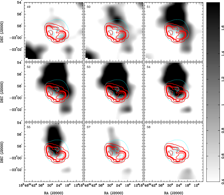
Figure 2.— The SRAO ¹²CO ($J$=1-0) intensity channel maps between 49 km s^-1 and 58 km s^-1 (smoothed to a resolution of $0.2^{\prime}$ by interpolation), overlaid with the 1.0–7.0 keV X-ray (cyan, thin) and 1.4 GHz radio (red, thick) continuum emission contours (from the NRAO VLA Sky Survey).

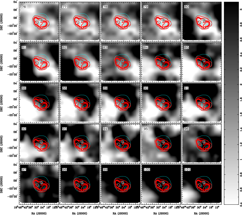
Figure 3.— The SRAO ¹²CO($J$=1-0) intensity channel maps between 76 km s^-1 and 101 km s^-1 (smoothed to a resolution of $0.2^{\prime}$ by interpolation), overlaid with the 1.0–7.0 keV X-ray (cyan, thin) and 1.4 GHz radio (red, thick) continuum emission contours (from the NRAO VLA Sky Survey).

We made the ¹²CO-emission intensity channel maps with $\sim 1$ km s^-1 velocity intervals. No evidence is found for the positional correlation between the first CO component and SNR Kes 75. However, the second and third components seem to have positional correlations with the remnant. Figures 2 and  3 show the ¹²CO channel maps in the intervals 49–58 km s^-1 and 76–101 km s^-1 (the main bodies of the second and third velocity components), respectively, with 1$\arcmin$ grid pointing. The channel maps are overlaid with the contours of the Chandra 1.0–7.0 keV X-ray and VLA 1.4 GHz radio continuum emission, respectively. In morphology, both the X-ray and radio emissions show bright half in the south and faint half in the north. It is interesting that the 49–58 km s^-1 cloud (as a part of the second component) is projectionally situated north to the radio- and X-ray-bright southern half of the SNR, seeming to cover the faint northern half. The CO emission around 51 km s^-1 also appears to surround the SNR from the north to the west. As parts of the third component of MC complex, the $V_{\rm LSR}\sim$ 83–96 km s^-1 MCs overlap a large north-western region of Kes 75, and the $\sim 97$–101 km s^-1 MCs completely overlap the remnant region (Fig. 3). The brightness anti-correlation between the two ¹²CO line components and the X-ray and radio (as well as mid-IR 24$\mu$m, §3.2) emissions is clear in a large scale.

3.2. The $V_{\rm LSR}\sim 54$ km s^-1 Molecular Cloud Component

Table 1Parameters of the Gaussian profile at $V_{\rm LSR}$=49-58 km s^-1 derived from the PMOD observation.

Line	Central velocity	Width of line	Mean Intensity
	(km s-1 )	(km s-1 )	(K)
12CO	53.7	3.7	3.16
13CO	53.6	3.3	0.44

In order to obtain detailed clues to the possible association of the cloud components with the SNR, we have analyzed the second and third velocity components in the inner $4.5^{\prime}\times 5^{\prime}$ area [centered at (${18}^{{\rm h}}{46}^{{\rm m}}{25}^{{\rm s}}.0,{-02}^{\circ}{59}^{\prime}{18}^{\prime\prime}$)] based on the PMOD observation.

Table 2Parameters for the MC derived from the PMOD observation.

Region	$V_{\rm LSR}$ interval	H2 column density	Virial mass	Molecular mass
	(km s-1 )	$N$(H2) (1020cm-2)	$M_{\rm vir}$ ($10^{3}M_{\odot}$)	$M$ ($10^{3}M_{\odot}$)
Main body	49–58	22.4 / 21.5	$26.6d_{10.6}$	$12.6d_{10.6}^{2}$ / $12.1d_{10.6}^{2}$
Southern region	45–58	14.8		$2.7d_{10.6}^{2}$
Gaussian around 54 km s-1		9.6		$1.8d_{10.6}^{2}$
Gaussian subtracted		5.2		$0.9d_{10.6}^{2}$

The observed parameters of the CO lines and the derived column density and cloud mass for the second velocity component (in interval 49–58 km s^-1) are summarized in Table 1 and Table 2, respectively. Two methods have been used in the derivation of the molecular column density and similar results are yielded. In the first method, the H₂ column density is calculated by adopting the mean CO-to-H₂ mass conversion factor $1.8\times 10^{20}$ cm^-2K^-1km^-1s (Dame et al. 2001; similar values also derived by Strong & Mattox 1996 and Hunter et al. 1997). In the second method, on the assumption of local thermodynamic equilibrium (LTE) and ¹²CO ($J$=1-0) line being optically thick, the ¹³CO column density is converted to the H₂ column density using $N$(H₂)/$N(^{13}$CO) $\approx 7\times 10^{5}$ (Frerking et al. 1982). In the estimate of the LTE mass of the molecular gas, a mean molecular weight per H₂ molecule $2.76m_{\rm H}$ has been adopted. Assuming the line of sight (LOS) size of the cloud similar to its apparent size $\sim 4^{\prime}$, we estimate the molecular density as $n({\rm H}_{2})\sim 60d_{10.6}^{-1}\,{\rm cm}^{-3}$, where $d_{10.6}=d/(10.6$ kpc) is the distance to the MC/SNR in units of the reference value (see §4.1 for the distance determination).

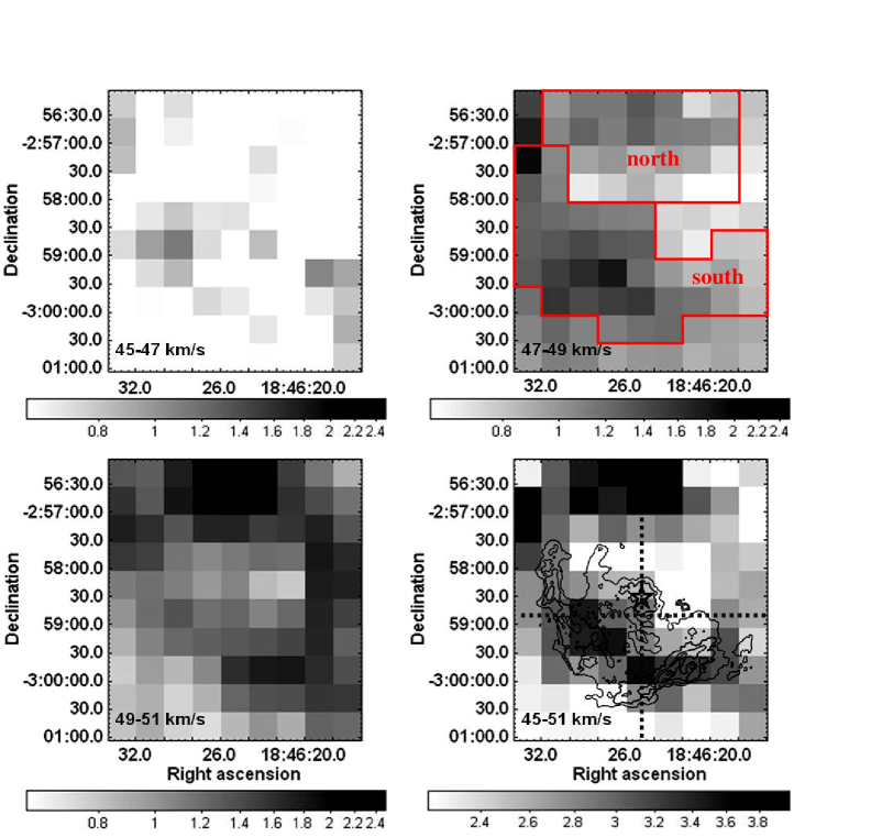
Figure 4.— The PMOD ¹²CO (J=1-0) intensity maps in the intervals 45–47, 47–49, 49–51, & 45–51 km s^-1. The two regions (6.5 arcmin² upper and 9 arcmin² lower) in the upper-right panel are defined for the CO-spectrum extraction. In the lower-right panel, the ¹²CO intensity map is overlaid with the 6 cm radio continuum contours (Becker & Helfand 1984), the star stands for the position of the pulsar, and the dotted lines indicate the E-W and N-S cuts for the PV diagrams (Fig. 6).

We extracted the ¹²CO and ¹³CO spectra in the velocity range 40–60 km s^-1 from two selected regions (as defined in Fig. 4), which basically correspond to the X-ray/IR/radio–bright southern half and faint northern half, respectively. The ¹²CO and ¹³CO spectra (shown in Fig. 5) in the both regions display a Gaussian profile around $V_{\rm LSR}\sim$54 km s^-1. There is a broad left wing (45–51 km s^-1) in the ¹²CO line profiles for both the northern and southern regions (as already seen in the spectrum for the entire remnant field, Fig. 1). Similar wing broadening is not seen in the ¹³CO lines. The $\sim 49$–58 km s^{-1 12}CO and ¹³CO Gaussian lines of the northern region are stronger than those of the southern region, indicating that the CO emission come majorly from the northern region, consistent with the ¹²CO channel maps (Fig. 2). However, the broadened left wing is not as strong in the northern region as in the southern one except in the interval 49–51 km s^-1. For the defined southern region, we obtain the mean integrated intensity spanning the line profile (45–58 km s^-1) $\sim$8.2 K km s^-1 and the corresponding molecular column density and gas mass as listed in Table 2. The contribution of the Gaussian component centered at 54 km s^-1 and the broadened part (with the Gaussian component subtracted) are also estimated, respectively, as given in Table 2.

Figure 5.— The 40–60 km s^-1 CO spectra from northern (6.5 arcmin², left) and southern (9 arcmin², right ) regions of SNR Kes 75 based on the PMOD observation. The thick and thin lines are for the ¹²CO($J$=1-0) and ¹³CO($J$=1-0) emission, respectively.

To better understand the velocity structure of the second ¹²CO component, we made the position-velocity (PV) diagrams (Fig. 6) along the east-west (E-W) and north-south (N-S) cuts centered at (${18}^{{\rm h}}{46}^{{\rm m}}{25}^{{\rm s}}.0,{-02}^{\circ}{58}^{\prime}{48}^{\prime\prime}$) (as labeled in Fig. 4). In Figure 6, it is clearly shown that the main body of the MC is located in the north of the Kes 75 area and the maximums of the ¹²CO line broadening appear near the edge (at radius about 1.7–$2^{\prime}$ from the pulsar) of the remnant.

The close-up ¹²CO channel maps and the integrated map in the blue-wing interval 45–51 km s^-1 are presented in Figure 4, in which the 6-cm radio continuum contours are superposed on the integrated map. In Figure 7 is shown a tri-color image of the Kes 75 area, with the ¹²CO intensity in the interval 45–51 km s^-1 in red, the Spitzer 24$\mu$m mid-IR intensity (together with the contours) in green, and the Chandra X-ray emission in blue. A cavity is revealed to be surrounded by a molecular shell in the line wing (45–51 km s^-1) intensity map, and, surprisingly, the shell in the south is coincident with the bright rim seen in the X-ray, mid-IR, and radio emissions. This shell is responsible for the maximums of the line broadening in the PV diagrams. The bright ¹²CO patch on the northern edge of the SNR may contain the contamination from the contribution of the main body of the $\sim 54$ km s^-1 MC at its Gaussian wing 49–$51$ km s^-1 (left panel of Fig.5), which has been seen to be located in the north (Fig.2 and Fig.6).

Figure 6.— Position-velocity diagrams along E-W cut (upper panel) and N-S cut (lower panel) [centered at (${18}^{{\rm h}}{46}^{{\rm m}}{25}^{{\rm s}}.0,{-02}^{\circ}{58}^{\prime}{48}^{\prime\prime}$)] based on the PMOD observation. Contour levels start from 1.0 K with in steps of 0.4 K. The dashed lines mark spatial the region of radius $1.7^{\prime}$ from the pulsar and the thick line marks 2.0^′ (see §4.2).

                      

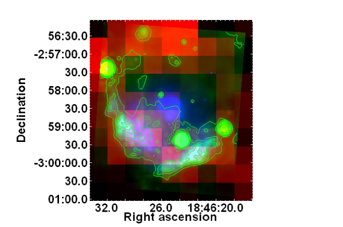
Figure 7.— Tri-color image of SNR Kes 75. The PMOD ¹²CO intensity map ($>2.2$ K km s^-1 or $11\sigma$) in the interval 45–51 km s^-1 is in red, the Spitzer 24$\mu$m mid-IR emission in green (including green contours), and the Chandra 1.0–7.0 keV X-rays (adaptively smoothed with the CIAO program csmooth to achieve a S/N ratio of 3) in blue. Each of the intensity maps is in logarithmic scales.

We did not find any CO feature between 60 km s^-1 and 110 km s^-1 (i.e. for the third molecular component) positionally coincident with the southern X-ray/mid-IR/radio–bright rim. The clouds in this velocity range are estimated to have a column density $N({\rm H}_{2})\sim 2.4\times 10^{22}$ cm^-2 in the northern region (as defined in Fig.4) and $\sim 1.9\times 10^{22}$ cm^-2 in the southern region (Fig.4).

Table 3Chandra X-ray Spectral Fits with 90% Confidence Ranges

Parameter	SE Clump	SW Clump	Northern Diffuse
$N_{H}$(1022cm-2)	$3.03^{+0.05}_{-0.13}$	$2.72^{+0.20}_{-0.17}$	$3.81^{+0.47}_{-0.32}$
$kT_{x}$(keV)	$0.65^{+0.03}_{-0.02}$	$0.88^{+0.30}_{-0.21}$
$Mg$	$1.26^{+0.18}_{-0.14}$	$1.04^{+0.24}_{-0.16}$
$Si$	$1.79^{+0.28}_{-0.26}$	$2.88^{+1.22}_{-0.83}$
$S$	$2.75^{+0.37}_{-0.40}$	$7.16^{+4.57}_{-2.36}$
$\tau$(1011s cm-3)	$4.12^{+1.23}_{-1.10}$	$0.35^{+0.10}_{-0.07}$
$norm$(10-2)	$1.36^{+0.35}_{-0.44}$	$0.18^{+0.19}_{-0.05}$
$PhoIndex$	$2.76^{+0.29}_{-0.14}$	$2.80^{+0.07}_{-0.07}$	$2.75^{+0.29}_{-0.20}$
$norm$ (10${}^{-3})$	$1.92^{+0.78}_{-0.51}$	$1.54^{+0.18}_{-0.14}$	$0.56^{+0.28}_{-0.14}$
$\chi_{r}^{2}$/dof	1.19/277	1.14/244	0.86/81
$N_{H}$(1022cm-2)	$3.23^{+0.02}_{-0.05}$	$3.55^{+0.08}_{-0.11}$
$kT_{x}$(keV)	$0.60^{+0.04}_{-0.03}$	$0.32^{+0.21}_{-0.06}$
$\tau$(1012s cm-3)	$>2.8$	$>1.0$
$norm$(10-2)	$1.84^{+0.28}_{-0.27}$	$3.97^{+2.81}_{-2.73}$
$kT_{x}$(keV)	$2.82^{+0.33}_{-0.27}$	$2.21^{+0.20}_{-0.20}$
$Mg$	$1.36^{+0.27}_{-0.26}$	$<0.42$
$Si$	$1.67^{+0.128}_{-0.16}$	$1.11^{+0.18}_{-0.16}$
$S$	$2.39^{+0.23}_{-0.34}$	$1.72^{+0.23}_{-0.25}$
$\tau$(1010s cm-3)	$3.53^{+0.36}_{-0.44}$	$3.41^{+0.56}_{-0.37}$
$norm$(10-3)	$2.78^{+0.47}_{-0.46}$	$3.35^{+0.57}_{-0.58}$
$\chi_{r}^{2}$/dof	1.15/277	1.26/244

3.3. X-ray Spectral Properties of Kes 75

To investigate the positional relation of the X-ray properties of SNR Kes 75 with the CO intensity distribution, we extracted three X-ray spectra of the southern clumpy shell and the faint northern diffuse emission (Fig. 8) from the reduced Chandra data using the CIAO3.4 script specextract. The background spectrum was extracted from a southeastern region outside the shell. The three on-source spectra are adaptively regrouped to achieve a background-subtracted signal-to-noise ratio (S/N) of 5 per bin. The previous Chandra X-ray studies by Helfand et al. (2003) and Morton et al. (2007) both used a uniform absorbing hydrogen column density $N_{H}$, fixed to that for the central PWN, for the entire remnant. Here we will allow $N_{H}$ to vary for each region in our spectral fit, in which the XSPEC11.3.2 software package with the Morrison & McCammon (1983) interstellar absorption is used.

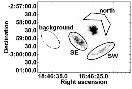
Figure 8.— The Chandra X-ray raw image of SNR Kes 75, labeled with the defined regions for the X-ray spectrum extraction. The point sources (except the central pulsar) detected with a wavelet source-detection algorithm have been removed.

Figure 9.— The Chandra-ACIS X-ray spectrum of the southeastern clump of Kes 75 (taken from a 183 ks data), fitted with the vnei (dashed line) plus power-law (dashed-dotted line) model. The dotted line around 3.12 keV is a Gaussian accounting for the Ar XVII line.

Figure 10.— The Chandra-ACIS X-ray spectrum of the northern region of Kes 75 (taken from a 183 ks data), fitted with a non-thermal power-law model.

The spectra of the two clumps along the southern shell contain distinct He$\alpha$ lines of Mg, Si, S, and Ar (see Fig.9 for the southeastern clump), as have been seen in the previous studies. However, the spectrum of the northern region appears to be featureless (Fig.10). The northern diffuse emission may be the dust-scattered light from the PWN; actually, Helfand et al. (2003) have pointed out that the effect of the dust-scattering halo of the Kes 75 PWN should be taken into account. Recently, Seward et al. (2006) clearly detected a dust-scattered X-ray halo around the Crab comprising 5% of the total strength, with surface brightness measured out to a radial distance of $18^{\prime}$. Therefore we fit the featureless spectrum of the northern region with a power-law model and, following Helfand et al. (2003), fit the spectra of the southern clumpy shell with a vnei + power-law model. As an alternative, we also fit the two spectra of the southern shell with a double-thermal-component model (accounting for the forward- and reverse-shocked gas), as Morton et al. (2007) did. The parameters of the fitting (with the 90% confidence ranges) are listed in Table 3.

The both models of our spectral fit generate a lower intervening hydrogen column density for the southern regions ($\leq 3.6\times 10^{22}$ cm^-2) than that used in the previous studies (fixed to the value for the PWN $\sim 4.0\times 10^{22}$ cm^-2). The northern diffuse emission has an intervening hydrogen column $N_{\rm H}\sim 3.5$–$4.3\times 10^{22}$ cm^-2, which seems higher than that for the southern regions. The column estimate for the southern regions from the vnei+powerlaw model, 2.6–$3.1\times 10^{22}$ cm^-2, is clearly lower than the column for the northern region. It is notable that the difference of $N_{H}$ between the northern region of the remnant (including the central PWN) and the southern regions in the case of using the vnei+powerlaw model is around $\sim 1\times 10^{22}$ cm^-2 (the differnce between the northern and southwestern regions is $1.1^{+0.5}_{-0.4}\times 10^{22}$ cm^-2 and that between the northern and southeastern regions is $0.8^{+0.5}_{-0.4}\times 10^{22}$ cm^-2). The both models produce elevated Si and S abundances. Using the volume emission measure, $fn_{e}n_{H}V$, derived from the normalization of the XSPEC model, we obtain an estimate for the hot-gas hydrogen-atom density $n_{H}\sim 5.4/1.4f^{-1/2}d_{10.6}^{-1/2}$ cm^-3 for the southeastern/southwestern regions, where $n_{e}$ is the electron density, $V$ is the volume of the emitting region, and $f$ is the volume filling factor of the hot gas ($0<f<1$). Here we have assumed $n_{e}\approx 1.2n_{H}$ and oblate spheroids ($24^{\prime\prime}\times 42^{\prime\prime}\times 42^{\prime\prime}$ and $19^{\prime\prime}\times 57^{\prime\prime}\times 57^{\prime\prime}$, respectively) for the defined southeastern and southwestern elliptical regions (Fig. 8). The mass of the southeastern/southwestern X-ray bright region is $\sim 3.4/1.7f^{1/2}d_{10.6}^{5/2}M_{\odot}$. The ionization timescales of the southeastern/southwestern X-ray–brighten regions in the vnei+powerlaw model thus imply ages of $\sim 2.0/0.6f^{1/2}d_{10.6}^{1/2}$ kyr, which are comparable with the spin-down timescale 723 yr (Gotthelf et al. 2000), considering factor $f$ is uncertain.

4. DISCUSSION

4.1. Association of SNR Kes 75 with the $V_{\rm LSR}\sim$54 km s^-1 MC and the Distance

From the above results of CO observations, we have obtained evidences for the association between SNR Kes 75 and the $V_{\rm LSR}\sim$54 km s^-1 MC. First, as seen in the ¹²CO spectra (Figs. 1 & 5), the broadened blue wing of the second (54 km s^-1) MC component indicates that the MC contains a part of gas that suffers a perturbation toward the observer. Similar one-sided broadened velocity-profiles are seen from a piece of MC in SNR CTB 109 (Fig. 2 in Sasaki et al. 2006) and the molecular arcs in SNR Kes 69 (Paper I). Secondly, the PV diagrams (Fig. 6) suggest that this blue-wing broadening takes place chiefly near the edge of the Kes 75 remnant. These characteristics hint that the 54 km s^-1 MC component may be perturbed by some interaction related with SNR Kes 75. Thirdly, the image of this broadening part is characterized by a shell-like structure surrounding a cavity, the southern part of which is coincident with the partial SNR shell seen in X-ray, mid-IR, and radio continuum (Figs. 4 and 7). This coincidence not only, again, demonstrates a consistent spatial position with that of the SNR, but also implies a shock interaction between the SNR and the molecular material (detailed in §4.2).

The establishment of the association of the $V_{\rm LSR}\sim$54 km s^-1 MC with SNR Kes 75 can provide an independent estimate for the kinematic distance to the SNR. Corresponding to the line center $V_{\rm LSR}\approx$54 km s^-1 of the unperturbed Gaussian profile (§3.2), there are two candidate kinematic distances to the MC along the LOS in the direction of Galactic longitude $l=29.7^{\circ}$. Using the rotation curve in Clements (1985), the two candidate distances are 3.3 and 10.6 kpc, which fall in the near and far side of the Sagittarius arm, respectively. Here we refer to the spiral model in Taylor & Cordes (1993; Fig. 1 therein) and adopt the circular rotation model with $R_{0}=8.0$ kpc (Reid 1993) and the constant circular velocity $V_{0}=220$ km s^-1. The tangent point in this direction is at $\sim 7.0$ kpc at the LSR velocity $\sim 103$ km s^-1. The HI observation reveals prominent absorption features at 68, 81, and 95 km s^-1 (e.g., LT08). Because these absorption features are seen at velocities greater than the systemic velocity, 54 km s^-1, of the MC associated with Kes 75, the SNR is located at the far side of the Sagittarius arm. This location is consistent with the lower limit, $\sim 5.1$ kpc, placed on the distance to this remnant by LT08 based on HI absorption. Thus, we determine the distance to be 10.6 kpc. As a consequence, the 60–110 km s^-1 MCs are all located in front of the 54 km s^-1 MC/Kes 75 association.

Our distance estimate is larger than the previous estimate of the upper limit, $\sim 7.5$ kpc, set by LT08, which suggests no HI absorption by the CO-line emitting cloud around 102 km s^-1 in the direction of Kes 75. The HI spectra in LT08 were extracted from two small regions which are bright in the radio continuum. To inspect the absorption in the larger radio-bright field, we made two-dimensional analysis of HI spectra along the Galactic latitude and longitude cuts near Kes 75, which are 3-pixels wide and cover most part of the radio-bright region (as shown in Fig. 11). We see in the produced HI PV diagrams that, above 95 km s^-1 at which the prominent HI absorption appears, there is a clear absorption feature at 100–103 km s^-1. Because of this feature, the HI absorption at $\sim 102$ km s^-1, although not strong, cannot be ignored, and this gas (at a distance of either 6.4 kpc or 7.5 kpc) is thus allowed to be located in the foreground of the SNR.

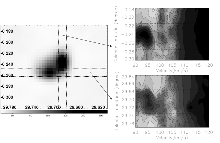
Figure 11.— The 1420 MHz continuum image (left) and the position-velocity diagrams of HI emission along the Galactic latitude (upper-right) and longitude (lower-right) cuts. In the two PV dragrams, HI emission is shown with contours at 20, 50, 70, 75, 82, 85, 88, 92, 98, 100, 110, and 120 and 10, 20, 30, 50, 70, 80, 84, 87, 90, 93, 96, 106, and 116 K, respectively, with the dark greyscale levels representing low brightness temperature. The dashed lines mark the spatial extent of the SNR. The rms noise of the PV diagrams is 1.15 K.

4.2. SNR physics of Kes 75

The discovery of the MC-SNR association and the updated distance to Kes 75 are helpful in understanding the remnant’s physical properties.

The SNR has a semicircular morphology in Chandra X-ray, 24$\mu$m mid-IR, and 1.4 GHz radio wavelengths. It might naturally have been suspected that the SNR interacts from the southern side, and slowed by, the huge MC. A similar scenario was suggested for SNR CTB 109, in which the SNR interacts with the western massive MC (Tatematsu et al. 1987; Wang et al. 1992; Rho & Petre 1997; Sasaki et al. 2004). In this case, for the young (§3.3) SNR Kes75, because of the drastic shock deceleration and hence the magnetic field compression and amplification, the radio emission might have been expected to be strong along the interface between the SNR and the MC. Also, because of the conversion of kinetic energy to the thermal energy, the X-rays might have been expected to be bright near the interface. In the CTB 109, the SNR is so evolved ($\sim 1\times 10^{4}$ yr) that the X-ray and radio emission have become faint along the border. The enhanced emissions are actually seen along the western rim of the middle age ($\sim 4$ kyr) SNR 3C391, where the blast wave has been suggested to hit a dense cloud plane (Chen et al. 2004). In Kes 75, however, the enhancement in either the radio or the X-ray emission does not appear along the northern edge of the apparent semicircle (if this edge were supposed as the interface).

An alternative possibility is that the SNR is located behind the MC and the X-ray of the northern half suffers severe extinction. In the latter case, however, since the effect of extinction by the cloud is negligible at the 1.4 GHz, the northern radio emission should be intrinsically faint. Therefore the SNR might propagate into a northern low-density region behind the MC, and this scenario thus explain why the remnant is also faint in the north in X-ray and mid-IR. It appears that faint 24$\mu$m mid-IR diffuse emission can marginally be discerned in the northern region (see Fig.12), but of course there may be confusion between the 24$\mu$m emission from the SNR itself and that from the larger molecular cloud region. In addition, a short, broken structure seems to be present in the 89 GHz radio image (Fig.3 in Bock & Gaensler 2005), coincident with the northern patch of the bright ¹²CO blue-wing emission (i.e., a weak CO-arc emission probably there, §3.2), namely, related to the northern maximum broadening in the CO PV maps (along the thick dashed line in Fig.6; §3.2). If this radio structure is a part of broken shell on the northern rim of the SNR, then this part of shell and the southern partial shell (in X-ray, IR, and radio) delineate a roughly circular morphology of the SNR.

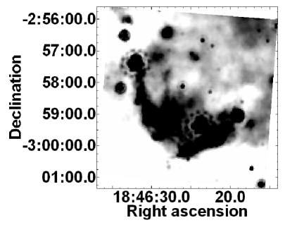
Figure 12.— The grey-scale Spitzer 24$\mu$m mid-IR image in logarithmic scales.

In the south, on the other hand, the partial SNR shell seen in these wavelengths has been shown to be coincident with the molecular shell in the blue wing of the 54 km s^-1 CO emission (Fig.7). The strong radio continuum emission may be generated from the SNR shock that is slowed by dense clouds (Frail & Mitchell 1998) or the blast wave that propagates in the intercloud material (Blandford & Cowie 1982). The molecular arc moving at a velocity $v_{m}$ of order 10 km s^-1 (implied by the blue-shifted line broadening which reflects the velocity component along the LOS), as a possibility, may represent the molecular gas that is perturbed by the slow transmitted cloud shock after it is struck by the blast wave. The position of the southern molecular shell may also indicate that some dense molecular gas may have been engulfed by the blast wave. The thermal X-ray emission may arise from the heated and evaporated gas (together with the ejecta) behind the shocked molecular gas, surrounding the engulfed clumps, or just behind the blast wave. In this scenario, there can be a crude pressure balance between the cloud shock and the X-ray emitting hot gas (Zel’dovich & Raizer 1967; McKee & Cowie 1975): $1.4n_{m}m_{H}v_{m}^{2}\sim 2.3n_{H}kT_{x}$, where $n_{m}$ is the number density of the hydrogen atoms ahead of the cloud shock, and $kT_{x}$ the temperature of the X-ray emitting gas (see Table 3; here the vnei+powerlaw model is used). Thereby $n_{m}\sim 4\times 10^{3}(n_{H}/3\,\mbox{cm}^{-3})(kT_{x}/0.8\,\mbox{keV})(v_{m}/10\,\mbox{km}\,\mbox{s}^{-1})^{-2}\,\mbox{cm}^{-3}$. This is over an order of magnitude higher than the mean density of the 54 km s^-1 main-body MC [$n({\rm H}_{2})\sim 60d_{10.6}^{-1}\,\mbox{cm}^{-3}$, §3.2]. The 24$\mu$m IR emission may come from the dust grains heated by the hot gas and even possibly from the shocked molecular gas (e.g., OH and H₂O).

In the above scenario, the dense molecular shell is pre-existing before the SNR shock arrives. The molecular shell could not be the material swept up by the supernova blast wave all the way to this radius ($r\sim 1.8^{\prime}\sim 6d_{10.6}$ pc). We adopt the observed total mass $\sim 2.7\times 10^{3}d_{10.6}^{2}M_{\odot}$ and the Gaussian-subtracted mass $\sim 0.9\times 10^{3}d_{10.6}^{2}M_{\odot}$ (Table 2) as the upper and lower limits of the mass of the southern molecular shell, respectively. If it were swept up by the blast wave, the original mean density of the molecular gas (counting a quarter of sphere of radius $1.8^{\prime}$) before it is swept up is $n_{0}({\rm H}_{2})\sim 60$–$180d_{10.6}^{-1}\,{\rm cm}^{-3}$ (the lower limit of the density is similar to the mean cloud density, §3.2). Based on the Sedov (1959) evolutionary law, if the blast-wave expansion velocity $v\sim 3.7\times 10^{3}\,{\rm km~{}s}^{-1}$ is adopted from the FWHM of the Si line (Helfand et al. 2003), the age of the remnant would be $\sim 0.4r/v\sim 640$ yr, seemingly close to the pulsar’s spin-down time scale 723 yr (Gotthelf et al. 2000). However, the explosion energy $E=(25/4\xi)\,2.8n_{0}(\mbox{H}_{2})m_{H}v^{2}r^{3}\sim 1.3\times 10^{54}[n_{0}(\mbox{H}_{2})/100\,\mbox{cm}^{-3}](v/3.7\times 10^{3}\,\mbox{km}\,\mbox{s}^{-1})^{2}(r/6\,\mbox{pc})^{3}$ ergs (where $\xi=2.026$), unreasonably higher than the canonical number $10^{51}$ ergs. On the other hand, the amount of hot gas in the southern clumps (contributing most to the thermal X-ray emission from the remnant), $\sim 5M_{\odot}$ (§3.3), is over two order of magnitudes smaller than that of the southern molecular shell. This would imply that massive swept-up molecular gas has quickly reformed after they were dissociated and ionized by the blast shock (at a velocity higher than $\sim 50$ km s^-1, Draine & McKee 1993). It seems impossible, however, because the timescale of H₂ gas formation, $\geq 10^{5.4}$ yr (Koyama & Inutsuka 2000), is much higher than the spin-down time (i.e., the remnant’s age).

We suggest that the pre-existing molecular shell may be the cooled, condensed, and clumpy material swept up by the stellar wind of the progenitor, which was in the vicinity of the large MC, in supplement to the above scenario of shock hitting the dense molecular gas. The presence of the central pulsar evidences that the Kes 75 SNR is the offspring of a core-collapse supernova explosion of a massive star. Massive stars may create a cavity with their energetic stellar winds and ionizing radiation before they explode, and the cavity wall may be an imprint of the wind modification left on the nearby environment. An excellent existing example of the molecular wind-bubble shells may be that recently discovered coincident with the ring nebula G79.29+0.46, which surrounds a luminous blue variable star (Rizzo et al. 2008), although it has a smaller radius ($\sim 1$ pc) and is at a higher kinetic temperature. As a matter of fact, in the case of Kes 75, a cavity is indeed seen surrounded by a molecular shell (§3.2; Fig.7). The scenario of the molecular shell of wind bubble also agrees with the suggestion of a strong Wolf-Rayet wind prior to the type Ib/c supernova event of Kes 75 (Chevalier 2005). In Kes 75, there seems not to be a red-shifted part of shell that expands backward and thus the wind-bubble may deviate from the spherical symmetry in the back side. To catch the essence, some parameters are estimated according to canonical bubble relation (Castor et al. 1975; Weaver et al. 1977), as a crude approximation, as below. The stellar wind bubble of the Kes 75 SNR progenitor has an age $\sim 5\times 10^{5}(r/6\,{\rm pc})^{5/3}L_{36}^{-1/3}[n({\rm H}_{2})/100\,{\rm cm}^{-3}]^{1/3}$ yr, where $L_{36}$ is the mechanical luminosity of the stellar wind in units of $10^{36}\,{\rm ergs}\,{\rm s}^{-1}$. The bubble shell expands at a velocity of $\sim 7(r/6\,{\rm pc})^{-2/3}L_{36}^{1/3}[n({\rm H}_{2})/100\,{\rm cm}^{-3}]^{-1/3}\,{\rm km~{}s}^{-1}$, a component of which projected to the LOS may be similar to the blueshift in the broadened line profile of the disturbed molecular gas. In addition, the wind-cavity wall scenario could not only naturally explain why the pre-shock molecular gas hitted by the SNR shock is over an order of magnitude denser than the main-body MC, but also avoid the above very high explosion energy by virtue of the low density (e.g., of order 0.1 cm^-3 for hydrogen atoms) in the cavity.

Similar scenario has been suggested to explain the physical properties of SNR Kes69, which bears resemblance with Kes 75 in that the molecular arcs are well coincident with the SNR shells and move at a velocity of order 10 km s^-1 (Paper I). In addition to Kes 69, a series of other SNRs have been suggested to be born in pre-existing stellar-wind cavities, with the shocks hitting the cavity walls, such as N132D (Hughes 1987; Chen et al. 2003), W49B (Keohane et al. 2007), and Kes 27 (Chen et al. 2008).

In combination of the blue-shifted broadening of the CO line profile, the SNR is suggested to be located proximately behind the 54 km s^-1 MC, and the molecular shell (in the broadened blue wing) was formed mainly on the near side close to the MC (i.e. toward the observer), as schetched in Figure 13. In the north, the remnant material expands into a tenuous region except for the side close to the MC, and the northern part of the SNR, together with the central PWN, is obscured by the MC complexes.

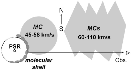
Figure 13.— Diagram showing the positional relation of SNR Kes 75 with the second and third MC complex components.

The extra obscuration in the northern area by the MCs could essentially account for the difference of $N_{H}$ ($\sim 1\times 10^{22}$ cm^-2) between the northern half of the remnant (including the central PWN) and the southern half (in the case in which vnei+powerlaw model is applied), as derived from the X-ray spectral analysis (§3.3). This explanation is fairly consistent with the difference of the molecular column density $\sim 1\times 10^{21}$ cm^-2 between the northern and southern areas for the second (40–60 km s^-1) molecular component and $\sim 5\times 10^{21}$ cm^-2 for the third (60–110 km s^-1) component (which is located in the foreground, see §4.1).

4.3. The High-energy Emission of PSR J1846-0258

McBride et al. (2008) find that the most unusual feature of PSR J1846-0258 is its large efficiency in converting spin-down power ($\dot{E}$) into X- and $\gamma$-ray luminosity ($L_{\rm 0.5-10keV}$ and $L_{\rm 20-100keV}$, respectively) of the PWN. In their work, the SNR distance of 19 kpc was used. If 10.6 kpc is adopted as the distance to the PSR, the 0.5–10 keV flux of the Kes 75 PWN $4.0\times 10^{-11}\,{\rm ergs~{}cm}^{-2}\,{\rm s}^{-1}$ (Helfand et al. 2003) corresponds to a luminosity $L_{\rm 0.5-10keV}\sim 5.4\times 10^{35}\,{\rm ergs~{}s}^{-1}$ and the X-ray efficiency is $L_{\rm 0.5-10keV}/\dot{E}\approx 6.4\%$. (The $\gamma$-ray efficiency is corrected to $L_{\rm 20-100keV}/\dot{E}\approx 4.8\%$.) The X-ray efficiency is lower than that ($9.1\%$) of PSR B0540$-$69 (Kaaret et al. 2001) and similar to that ($5.1\%$) of the Crab [here $L_{\rm 0.2-10keV}\sim 3.3\times 10^{37}\,{\rm ergs~{}s}^{-1}$ (Kaaret et al. 2001) is converted to $L_{\rm 0.5-10keV}\sim 2.4\times 10^{37}\,{\rm ergs~{}s}^{-1}$ for the Crab Nebula with the X-ray photon index 2.1 (Willingale et al. 2001)], and thus the efficiency seems to be not peculiar among the young pulsars.

The High Energy Stereoscopic System (H.E.S.S.) collaboration (Djannati-Atai et al. 2007) discovers the very high energy (VHE) emission from the sky region of SNR Kes 75 and regards it as a point-like source with the point spread function (PSF) $5^{\prime}$, which is in a quite good agreement with the position of the PSR J1846-0258. It is noted that $L_{x}/L{\gamma}\sim$ 10 for the case of Kes 75, only one-third of SNR G21.5$-$0.9 and one-twelfth of the Crab Nebula. This seems to imply a $\gamma$-ray excess in Kes 75 comparing to other plerions. Since the H.E.S.S. VHE observation cannot resolved the PWN from other structures of Kes 75, whose apparent size $4^{\prime}$ is smaller than the PSF, the $\gamma$ excess cannot be excluded to arise from other sites than the PWN. The discovery of the association of Kes 75 with the MC provides a possible interpretation for this excess, because a part of the $\gamma$-rays may come from the decay of neutral pions produced by proton interactions between the SNR shock and the MC.

5. CONCLUSIONS

Millimeter observations of the molecular gas toward SNR Kes 75 have been made in SRAO and PMOD. By the spectroscopic analysis of the ¹²CO (J=1-0) emission, in combination with the X-ray, 24$\mu$m mid-IR, and radio continuum data, we conclude the main results as follows.

1. There are several CO emission peaks in a broad LSR velocity range from 3 to 110 km s^-1. The $\sim 83$–96 km s^-1 MCs overlap a large north-western region of the remnant and is inferred to be located in the foreground of the SNR. The 45–58 km s^-1 molecular gas shows a blue-shifted broadening in the ¹²CO line profile and the intensity centroid of the gas sits in the northern area of the SNR. The position-velocity map displays maximums of line broadening near the edge of the remnant.

2. In the integrated intensity map of the broadened blue wing at 45–51 km s^-1, a cavity surrounded by a molecular shell is unveiled, which is coincident with the SNR, and the shell in the south follows the bright partial shell seen in X-rays, mid-IR, and radio continuum.

3. All the observational features of the broadened blue wing provide effective evidences that Kes 75 is associated with the adjacent 10${}^{4}M_{\odot}$ 54 km s^-1 MC.

4. The establishment of the association between Kes 75 and the 54 km s^-1 MC results in a determination of the kinematic distance at $\sim 10.6\,{\rm kpc}$ to the remnant, which agrees with a location at the far side of the Sagittarius arm.

5. The X-ray, mid-IR, and radio shell-like morphology in the south can be accounted for by the SNR shock striking a pre-existing molecular shell. This shell may represent the debris of the cooled, condensed, clumpy shell of the progenitor’s wind-bubble proximately behind the 54 km s^-1 cloud.

6. The discovery of the association of Kes 75 with MC can provide a qualitative explanation for the $\gamma$-ray excess of the remnant.

References

- Becker & Helfand (1984) Becker, R. H., & Helfand, D. J. 1984, ApJ, 283, 154
- Blandford et al. (1982) Blandford, R. D., & Cowie, L. L. 1982, ApJ, 260, 625
- Blanton & Helfand (1996) Blanton, E. L., & Helfand, D. J. 1996, ApJ, 470, 961
- Bock & Gaensler (2005) Bock, D. C.-J., & Gaensler, B. M. 2005, ApJ, 626, 343
- Caselli (2002) Caselli, P, Benson, P. J., Myers, P. C., & Tafalla, M. 2002, ApJ, 572, 238
- Castor (75) Castor, J., McCray, R., & Weaver, R. 1975, ApJ, 200, L107
- Caswell (1975) Caswell, J. L., Murray, J. D., Roger, R. S., Cole, D. J., & Cooke, D. J. 1975, A&A, 45, 239
- Chen et al. (2008) Chen, Y., Seward, F. D., Sun, M., & Li, J.-T. 2008, ApJ, 676, 1040
- Chen (2001) Chen, Y, & Slane, P. O. 2001, ApJ, 563, 202
- Chen (2004) Chen, Y., Su. Y., Slane. P. O., & Wang, Q. D. 2004, ApJ, 616, 885
- Chen (2003) Chen, Y., Zhang, F., Williams, R. M., & Wang, Q. D. 2003, ApJ, 595, 227
- Chevalier (2005) Chevalier, R. G. 2005, ApJ, 619, 839
- Clemens (1985) Clemens, D. P. 1985, ApJ, 295, 422
- Dame et al. (1986) Dame, T. M., Elmegreen, B. G., Cohen, R. S., & Thaddeus, P. 1986, ApJ, 305, 892
- Dame et al. (2001) Dame, T. M., Hartmann, D., and Thaddeus, P. 2001, ApJ, 547, 792
- Djannati-Atai (2007) Djannati-Atai. A., De Jager, O. C., Terrier, R., Gallant, Y. A., Hoppe, S. (H.E.S.S. Collaboration) 2007, 30th ICRC (arXiv: 0710.2247)
- Draine & McKee (1993) Draine, B. T. & McKee, C. F. 1993, ARA&A, 31, 373
- Frail et al. (1996) Frail, D. A., Goss, W. M., Reynoso, E. M., Giacani, E. B., Green, A. J., & Otrupcek, R. 1996, AJ, 111, 1651
- Frail et al. (1998) Frail, D. A. & Mitchell, G. F. 1998, ApJ, 508, 690
- Frerk et al. (1982) Frerking, M. A., Langer, W. D., & Wilson, R. W. 1982, ApJ, 262, 590
- Gotthelf et al. (2000) Gotthelf, E. V., Vasisht, G., Boylan-Kolchin, M., & Torii, K. 2000, ApJ, 542, L37
- Helfand et al. (2003) Helfand, D. J., Collins, B. F., & Gotthelf, E. V. 2003, ApJ, 582, 783
- Huang & Thaddeus (1986) Huang, Y.-L., & Thaddeus, P. 1986, ApJ, 309, 804
- Hughes (1987) Hughes, J. P. 1987, ApJ, 314, 103
- Hunter (1997) Hunter, S. D. et al. 1997, ApJ, 481, 205
- Kaaret (2001) Kaaret, P., Marshall, H. L., Aldcroft, T. L., Graessle, D. E., Karovska, M., Murray, S. S., Rots, A. H., Schulz, N. S., Seward, F. D. 2001, ApJ, 56, 1159
- Keohane et al. (2007) Keohane, J. W., Reach, W. T., Rho, J., & Jarrett, T. H. 2007, ApJ, 654, 938
- Koyama & Inutsuka (2000) Koyama, H. & Inutsuka, S.-I. 2000, ApJ, 532, 980
- Kumar (2008) Kumar, H. S., & Safi-Harb, S. 2008, ApJ, 678, L43
- Leahy (2008) Leahy, D. A., & Tian, W.W . 2008, A&A, 480, L25 (LT08)
- McBride (2008) McBride, V. A., Dean, A. J., & Bazzano. F. 2008, A&A, 477, 249
- Milne (1979) Milne, D. K. 1979, AuJPh, 32, 83
- McKee (1975) McKee, C.F. & Cowie, L.L. 1975, ApJ, 195, 715
- Morroson (1988) Morrison, R., & McCammon, D. 1983, ApJ, 270, 119
- Morton (2007) Morton, T. D., Slane, P., Borkowski, K. J., Reynolds, S. P., Helfand, D. J., Gaensler, B. M., & Hughes, J. P. 2007, ApJ, 667, 291
- Ng (2008) Ng, C.-Y., Slane, P. O., Gaensler, B. M., & Hughes, J. P. 2008, submitted to ApJ, arXiv:0804.3384
- Reid (1993) Reid, M. J. 1993, ARA&A, 31, 345
- Rho (1996) Rho, J. H., & Petre, R. 1996, ApJ, 467, 698
- Rho (1997) Rho, J. H., & Petre, R. 1997, ApJ, 484, 828
- Rieke et al. (2004) Rieke, G. H. et al. 2004, ApJS, 154, 25
- Rizzo (2008) Rizzo, J. R., Jimenez-Esteban, F. M., & Ortiz, E. 2008, ApJ, 681, 355
- Sasaki (2004) Sasaki, M., Plucinsky, P. P., Gaetz, T. J., Smith, R. K., Edgar, R. J., & Slane, P. O. 2004, ApJ, 617, 322
- Sasaki (2006) Sasaki, M, Kothes, R., Plucinsky, P. P., Gaetz, T. J., Brunt, C. M. 2006, ApJ, 642, L149
- Sedov (1959) Sedov, L. I. 1959, Similarity and Dimensional Methods in Mechanics (New York: Academic)
- Seward (2006) Seward, F. D., Gorenstein, P., & Smith, R. K. 2006, ApJ, 636, 873
- Stil (2006) Stil, J. M., Taylor, A. R., Dickey, J. M., Kavars, D. W., Martin, P. G., Rothwell, T. A., Boothroyd, A. I., Lockman, F. J., & McClure-Griffiths, N. M. 2006, AJ, 132, 1158
- Strong (1996) Strong, A. W., & Mattox, J. R. 1996, A&A, 308, L21
- Tatematsu (1987) Tatematsu, K., Fukui, Y., Nakano, M., Kogure, T., Ogawa, H., & Kawabata, K. 1987, A&A, 184, 279
- Taylor & Cordes (1993) Taylor, J. H., & Cordes, J. M. 1993, ApJ, 411, 674
- Wang (91) Wang, Z. R., Qu, Q.Y., Luo, D., McCray, R., & Mac Low, M. M. 1992, ApJ, 388, 127
- Weaver (77) Weaver, R., McCray, R., Castor, J., Shapiro, P., & Moore, R. 1977, ApJ, 218, 377
- (52) Willingale, R., Aschenbach, B., Griffiths, R. G., Sembay, S., Warwick, R. S., Becker, W., Abbey, A. F., & Bonnet-Bidaud, J.-M. 2001, A&A, 365, L212
- Wilner (98) Wilner, D. J., Reynolds, S. P., Moffett, D. A. 1998, ApJ, 115, 247
- Zel’dovich (67) Zel’dovich, Ya. B. & Raizer, Yu. M. 1967, Physics of shock waves and high-temperature hydrodynamic phenomena (New York: Academic Press)
- Zhou (08) Zhou, X., Chen, Y., Su, Y., & Yang, J. 2008, ApJ, accepted, arXiv:0809.4306 (Paper I)