Abstract

Energy losses of fast color particles in random inhomogeneous color medium created in high energy nuclear collisions are estimated.

1 Introduction

Experimental [1, 2] and theoretical [3, 4] studies of energy loss of fast particles provide an extremely valuable option of a quantitative assessment of properties of dense strongly interacting medium created in ultrarelativistic heavy ion collisions. In such high energy nuclear collisions a transformation of incident dense partonic fluxes into a final set of inelastically produced hadrons proceeds through initial energy release via creation of physical partonic modes followed by their transformation into a high density hadronic system that finally takes form of free-streaming hadrons that are observed experimentally. Detailed dynamical description of high energy nuclear collisions is an extremely difficult task, so theoretical simplifications and/or complicated Monte Carlo models are needed to describe the results of existing experiments and predict those of future ones. The main issue addressed in such modeling is a relative role of parton phase contribution versus the hadron phase one. One of generic features of a parton phase picture describing dynamics of semihard partonic degrees of freedom is a pronounced turbulence-like inhomogeneity of energy release in the impact parameter plane on the event-by-event basis [5] having its origin in the powerlike nature of the cross sections of partonic interactions. Therefore, when considering the parton phase contribution to the energy loss of fast particles, understanding the effect of these inhomogeneities is very important.

In the present paper we shall consider this problem in the simplest setting [6, 7] in which the energy loss is computed, in the quasi-abelian approximation, as the work done on the incident particle by the field it induces in the medium [8]. In this approach the origin of the losses is a nonzero imaginary part of dielectric permittivity of the medium. In the case of random inhomogeneous medium there appears a new contribution to this imaginary part. The physical mechanism of energy loss in the randomly inhomogeneous medium leading to an appearance of such inhomogeneity-induced imaginary part of dielectric permittivity can be described as a scattering of the Weizsaker-Williams modes of the proper field of the incident particle on the inhomogeneities in the medium. Depending on the stochastic properties of the medium some modes can become resonant resulting in transition and Cherenkov radiation, see e.g. [9]. In the light of discussions on possible observation of gluon Cherenkov radiation at RHIC, see e.g. [10, 11], of special interest is the fact that the inhomogeneity-induced losses are significantly amplified in the medium in which the effective permeability exceeds the Cherenkov threshold [9]. Let us note that the problem of energy loss in the random inhomogeneous medium has deep links [12] with that of wave propagation in random media, see e.g. the review [13].

2 Energy loss

The average energy losses per unit length of ultrarelativistic particle moving along the $z$ axis are described by an appropriate generalization [6, 7] of the standard formula [8]:

$$\frac{dW}{dz}=gQ^{a}\hat{\bf z}\,\langle{\bf E}^{a}({\bf r},t)\rangle_{{\bf r}=\hat{\bf z}t}$$ (1)

where $g$ is a color charge, $Q^{a}$ is a color spin normalized at quadratic Casimir invariants of SU(3) for fundamental (adjoint) representations $C_{F(V)}$ , $Q^{a}Q^{a}=C_{F(V)}$, for the projectile quark or gluon respectively and $\langle{\bf E}^{a}({\bf r},t)\rangle$ is a chromoelectric field created in the medium by the propagating particle averaged over the fluctuations of random inhomogeneous medium.

In the case of inhomogeneous medium the local fluctuations of its properties are customarily parametrized by the coordinate-dependent chromodielectric permittivity $\varepsilon^{ab}({\bf r})$. For given configuration of $\varepsilon^{ab}({\bf r})$ the spectral component of the chromoelectric field is determined from the abelianized equations of motion for the chromoelectric field:

$$\triangle{\bf E}^{a}-\nabla\left(\nabla{\bf E}^{a}\right)+\omega^{2}\,\varepsilon({\bf r})\,{\bf E}^{a}\,=4\pi\imath\omega j^{a}(\omega,{\bf r})$$ (2)

where $j^{a}(\omega,{\bf r})$ is a spectral component of the external current and we have assumed a diagonal structure of chromodielectric permittivity, $\varepsilon^{ab}({\bf r})=\varepsilon({\bf r})\,\delta^{ab}$. In the considered case of uniformly moving ultrarelativistic particle one has ${\bf j}^{a}(\omega,{\bf k})=2\pi gQ^{a}\hat{\bf z}\delta(\omega-k_{z})$. Random inhomogeneities can conveniently be parametrized by explicitly identifying the non-random and random contributions to dielectric permittivity:

$$\varepsilon({\bf r})\,=\,\varepsilon_{0}\left(1+\xi({\bf r})\right)$$ (3)

where $\xi({\bf r})$ is a random contribution to permittivity having zero mean $\langle{\xi(\bf r})\rangle=0$. In what follows we shall consider the simplest case of Gaussian ensemble so that $\xi({\bf r})$ are fully characterized by the binary correlation function

$$\langle\xi\left({\bf r}_{1}\right)\xi\left({\bf r}_{2}\right)\rangle=g\left(|{\bf r}_{1}-{\bf r}_{2}|\right)$$ (4)

It is well known, see e.g. [9, 13], that taking into account the random inhomogeneities leads to an equation for the average electric field containing a tensor of effective dielectric permittivity $\varepsilon_{ij}(\omega,{\bf k})$ having nontrivial imaginary parts that depend on the statistical properties of fluctuations $\xi({\bf r})$:

$$\left[\varepsilon_{ij}(w,\mathbf{k})-\frac{k^{2}}{w^{2}}\left(\delta_{i,j}-\frac{k_{i}k_{j}}{k^{2}}\right)\right]\langle E^{a}_{j}(w,\mathbf{k})\rangle=\frac{4\pi}{\imath\,w}j^{a}_{i}(w,\mathbf{k})$$ (5)

where we have introduced a notation $w=\sqrt{\varepsilon_{0}}\omega$. Averaging over the stochastic ensemble of random inhomogeneities introduces an implicit dependence on its characteristics, e.g. on correlation radius $r_{c}$ and fluctuation magnitude $\sigma$, so that one should in fact write $\varepsilon_{ij}(w,\mathbf{k}|\,r_{c},\sigma)$. It is convenient to explicitly introduce the transverse and longitudinal components $\varepsilon_{t}$ and $\varepsilon_{l}$:

$$\varepsilon_{ij}(w,{\bf k}|\,r_{c},\sigma)\equiv\left(\delta_{ij}-\frac{k_{i}k_{j}}{k^{2}}\right)\varepsilon^{t}(w,{\bf k}|\,r_{c},\sigma)+\frac{k_{i}k_{j}}{k^{2}}\varepsilon^{l}(w,{\bf k}|\,r_{c},\sigma)$$ (6)

In terms of the decomposition (6) the expression for the energy losses takes, for some given $\varepsilon_{ij}(\omega,{\bf k}|\,r_{c},\sigma)$, the form

$$\frac{dW}{dz} = \frac{g^{2}C_{F(V)}}{2\pi^{2}}\int d^{3}k\left\{\frac{w}{k^{2}}\left[{\rm Im}\,\frac{1}{\varepsilon^{l}(w,{\bf k}|\,r_{c},\sigma)}\right.\right.$$ (7)

$$- \left.\left.\left(w^{2}-k^{2}\right){\rm Im}\,\frac{1}{w^{2}\varepsilon^{t}(w,{\bf k}|\,r_{c},\sigma)-k^{2}}\right]\right\}_{w=k_{z}}$$

Let us now consider the particular case of an exponential binary correlation function

$$g(r)=\sigma^{2}e^{-r/r_{c}}$$ (8)

that allows an explicit analytical computation of $\varepsilon_{ij}(\omega,{\bf k})$ to all orders in $\sigma$ in the one-loop approximation corresponding to the regime $\sigma^{2}(wr_{c})\ll 1$, see Appendix. The corresponding calculation is naturally performed in terms of the polarization tensor $\Pi_{ij}(w,{\bf k})$ related to chromodielectric permittivity by the following relation:

$$\varepsilon_{ij}(w,{\bf k}|\,r_{c},\sigma)=\varepsilon_{0}\left(1-\frac{1}{w^{2}}\Pi_{ij}(w,{\bf k}|\,r_{c},\sigma)\right)$$ (9)

The decomposition of chromodielectric permittivity (6) leads to the corresponding decomposition of the polarization tensor. The explicit expressions for the transverse and longitudinal components of the polarization tensor $\Pi_{ij}(w,{\bf k}|\,r_{c},\sigma)$ computed in the one-loop approximation read, cf. Eqs. (20) and (21) in the Appendix:

$$\Pi^{t}(w,{\bf k}|\,r_{c},\sigma) = \sigma^{2}w^{2}\left[\frac{w^{2}}{(w+i\delta)^{2}-k^{2}}-\frac{\delta(\delta+iw)}{2k^{2}}\right.$$ (10)

$$+ \left.\frac{\delta^{2}+w^{2}+k^{2}}{k^{2}}\frac{\delta}{k}\arctan\left(\frac{ik}{w+i\delta}\right)\right]$$

and

$$\Pi^{l}(w,{\bf k}|\,r_{c},\sigma) = \sigma^{2}w^{2}\left[1+\frac{\delta(\delta+iw)}{2k^{2}}\right.$$ (11)

$$- \left.\frac{\delta^{2}+w^{2}+k^{2}}{k^{2}}\frac{\delta}{k}\arctan\left(\frac{ik}{w+i\delta}\right)\right]\,,$$

where $\delta=1/r_{c}$. Let us stress once again that even if the non-random chromodelectric permittivity $\varepsilon_{0}$ does not have a significant imaginary part so that the corresponding energy losses determined by (7) are absent, the effective chromodielectric permittivity determined by (10,11) has a nontrivial imaginary part and, therefore, there arise specific energy losses directly related to the random fluctuations in the medium in which they propagate.

Let us now estimate the magnitude of the above-described stochastic energy loss. In presenting the results it turns out convenient to rewrite the expression for the energy loss (7) in the form:

$$\frac{dW}{dz}=C_{F(V)}\frac{\alpha_{s}}{\pi}\frac{1}{r_{c}^{2}}\left[f_{t}(pr_{c}|\,\sigma,\varepsilon_{0})+f_{l}(pr_{c}|\,\sigma,\varepsilon_{0})\right]$$ (12)

where $p$ is an energy of the incident quark (gluon) and the dimensionless functions $f_{t}(pr_{c}|\,\sigma,\varepsilon_{0})$ and $f_{l}(pr_{c}|\,\sigma,\varepsilon_{0})$ quantify the transverse and longitudinal energy losses correspondingly. The dependence on $p$ appeared through cutting the momentum integration in (7) at $p$ at the upper limit. The physical meaning of this cutoff is that within the adopted scheme of calculating the energy losses we should restrict our consideration to the soft modes in the proper field of the incident particle.

In considering transverse contribution to the energy losses it is important to distinguish between the cases of $\varepsilon_{0}<1$ (below the Cherenkov threshold) and $\varepsilon_{0}>1$ (above the Cherenkov threshold).

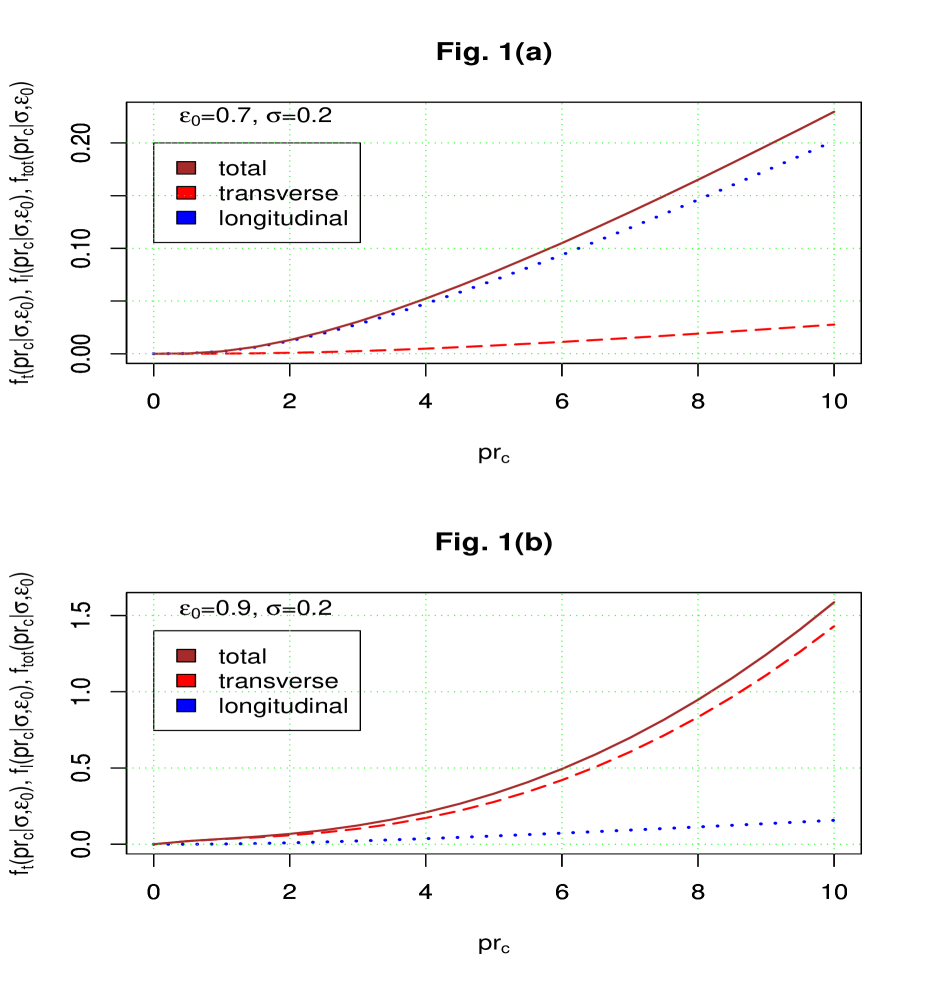
Figure 1: Transverse losses $f_{t}(pr_{c}|\,\sigma,\varepsilon_{0})$ (red, dashed), longitudinal losses $f_{l}(pr_{c}|\,\sigma,\varepsilon_{0})$ (blue, dotted) and total losses $f_{\rm tot}(pr_{c}|\,\sigma,\varepsilon_{0})$ (brown, solid), $\sigma=0.2$: (a) for $\varepsilon_{0}=0.7$; (b) for $\varepsilon_{0}=0.9$.

In the first case of $\varepsilon_{0}<1$ the transverse losses are purely stochastic so that they vanish at vanishing fluctuation strength $\sigma$, $f_{t}(pr_{c}|\,\sigma\to 0,\varepsilon_{0})\to 0$. An interesting feature of the stochastic energy loss in this regime is a dependence of the relative weight of transverse and longitudinal contributions from the value of $\varepsilon_{0}$. At small $\varepsilon_{0}$ longitudinal losses dominate over transverse ones while for $\varepsilon_{0}\lesssim 1$ the transverse losses are dominant. This is illustrated in Fig. 1 in which we plot the dependence of transverse $f_{t}(pr_{c}|\,\sigma,\varepsilon_{0})$ and longitudinal $f_{l}(pr_{c}|\,\sigma,\varepsilon_{0})$ stochastic losses on $pr_{c}$ for $\varepsilon=0.7$, where longitudinal losses dominate, and $\varepsilon=0.9$, where transverse losses substantially exceed the longitudinal ones.

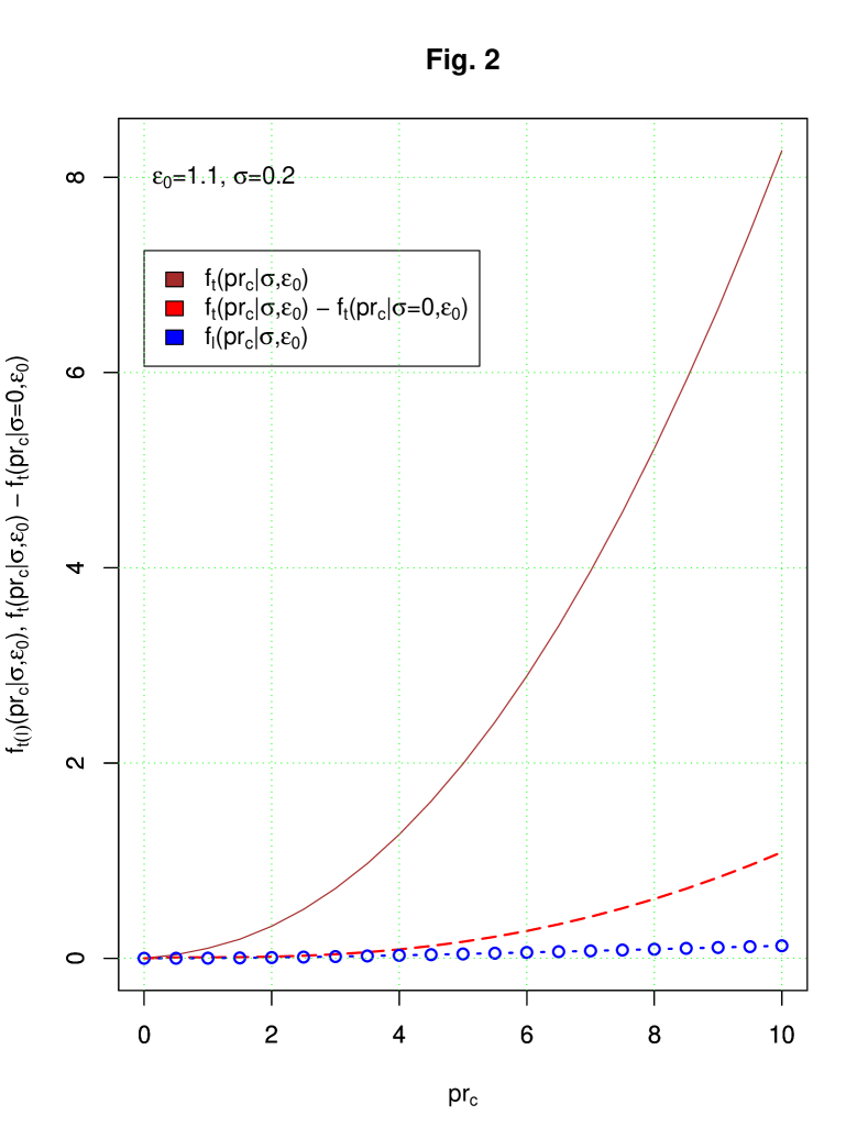
Figure 2: Full transverse losses $f_{t}(pr_{c}|\,\sigma,\varepsilon_{0})$ (brown, solid), stochastic contribution to transverse losses $f^{\rm stoch}_{t}(pr_{c}|\,\sigma,\varepsilon_{0})=f_{t}(pr_{c}|\,\sigma,\varepsilon_{0})-f_{t}(pr_{c}|\,\sigma=0,\varepsilon_{0})$ (red, dashed) and longitudinal losses $f_{l}(pr_{c}|\,\sigma,\varepsilon_{0})$ (blue, dotted), $\sigma=0.2$, $\varepsilon_{0}=1.1$.

In the second case of $\varepsilon_{0}>1$ the transverse losses are nonzero even at vanishing fluctuation strength $\sigma\to 0$ due to Cherenkov radiation. In the considered simplest case of constant energy-independent imaginary part of $\varepsilon_{0}$ the Cherenkov contribution to the transverse losses is very big: it is in fact quadratically divergent at the upper limit of energy integration. Therefore to consider the stochastic contribution to energy losses in the Cherenkov regime one has to subtract the pure Cherenkov losses from the full transverse ones. The stochastic contribution $f^{\rm stoch}_{t}(pr_{c}|\,\sigma,\varepsilon_{0})$ to transverse energy loss in this case is thus just $f^{\rm stoch}_{t}(pr_{c}|\,\sigma,\varepsilon_{0})=f_{t}(pr_{c}|\,\sigma,\varepsilon_{0})-f_{t}(pr_{c}|\,\sigma=0,\varepsilon_{0})$. The full transverse loss $f_{t}(pr_{c}|\,\sigma,\varepsilon_{0})$, its stochastic component $f^{\rm stoch}_{t}(pr_{c}|\,\sigma,\varepsilon_{0})$ and the longitudinal loss $f_{l}(pr_{c}|\,\sigma,\varepsilon_{0})$ are plotted in Fig. 2 for $\varepsilon=1.1$. We see that the pure Cherenkov contribution $f_{t}(pr_{c}|\,\sigma=0,\varepsilon_{0})$ is clearly dominant while the stochastic losses $f^{\rm stoch}_{t}(pr_{c}|\,\sigma,\varepsilon_{0})$ and $f_{l}(pr_{c}|\,\sigma,\varepsilon_{0})$ are similar to those for $\varepsilon_{0}=0.9$ plotted in Fig. 1(b).

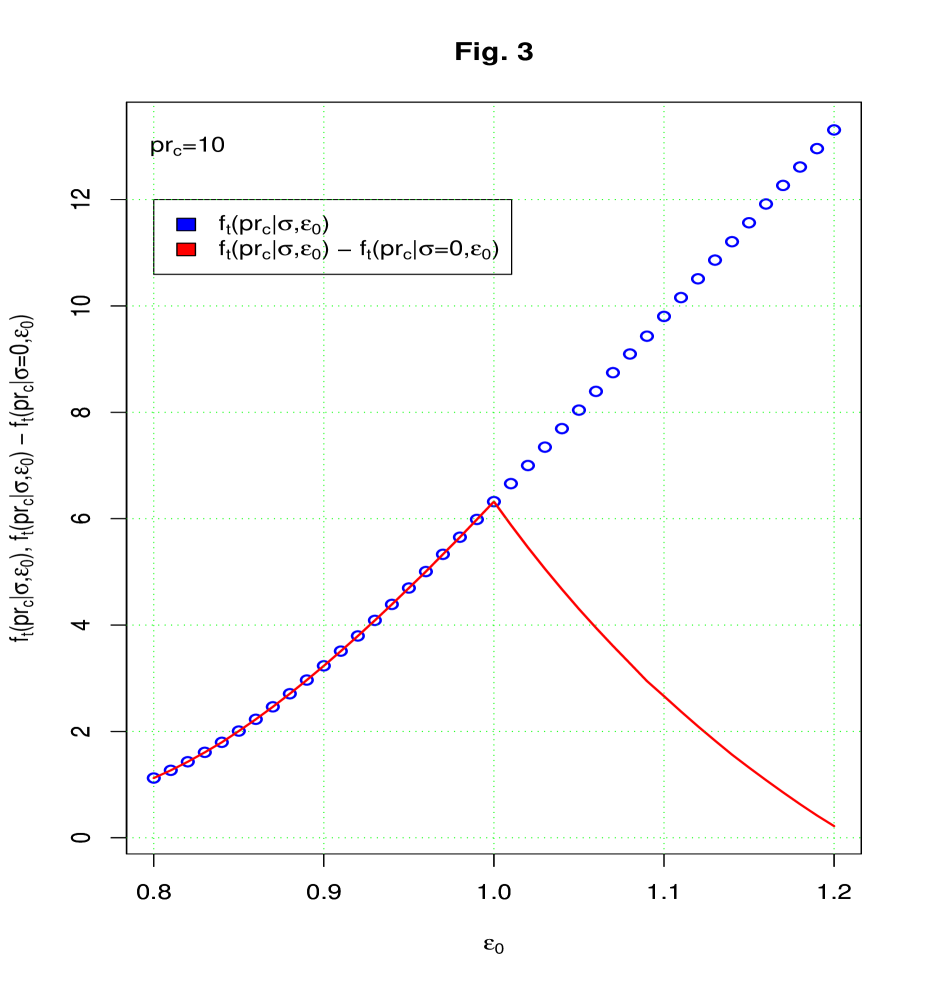
Figure 3: Dependence of full transverse losses $f_{t}(pr_{c}|\,\sigma,\varepsilon_{0})$ (blue, dotted) and stochastic contribution to transverse losses $f^{\rm stoch}_{t}(pr_{c}|\,\sigma,\varepsilon_{0})=f_{t}(pr_{c}|\,\sigma,\varepsilon_{0})-f_{t}(pr_{c}|\,\sigma=0,\varepsilon_{0})$ (red, solid) on the bare dielectric permittivity $\varepsilon_{0}$, $\sigma=0.2$, $pr_{c}=10$.

The dependence of transverse losses $f_{t}(pr_{c}|\,\sigma,\varepsilon_{0})$ and stochastic transverse losses $f^{\rm stoch}_{t}(pr_{c}|\,\sigma,\varepsilon_{0})$ on $\varepsilon_{0}$ is plotted, for $\sigma=0.2$ and $pr_{c}=10$, in Fig. 3. We see that a relative weight of stochastic losses above the Cherenkov threshold is diminishing with growing $\varepsilon_{0}$.

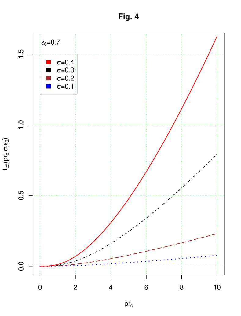
Figure 4: Dependence of total losses $f_{\rm tot}(pr_{c}|\,\sigma,\varepsilon_{0})$ on $pr_{c}$ for $\sigma=0.1$ (blue, dotted); $\sigma=0.2$ (brown, dashed); $\sigma=0.3$ (black, dashed-dotted); $\sigma=0.4$ (red, solid) for $\varepsilon_{0}=0.7$.

The dependence of total losses $f_{\rm tot}(pr_{c}|\,\sigma,\varepsilon_{0})$ on the fluctuation magnitude $\sigma$ is illustrated by plotting the dependence on $pr_{c}$ for several values of $\sigma$ in Fig. 4 for $\varepsilon_{0}=0.7$. As expected, the losses grow with growing $\sigma$.

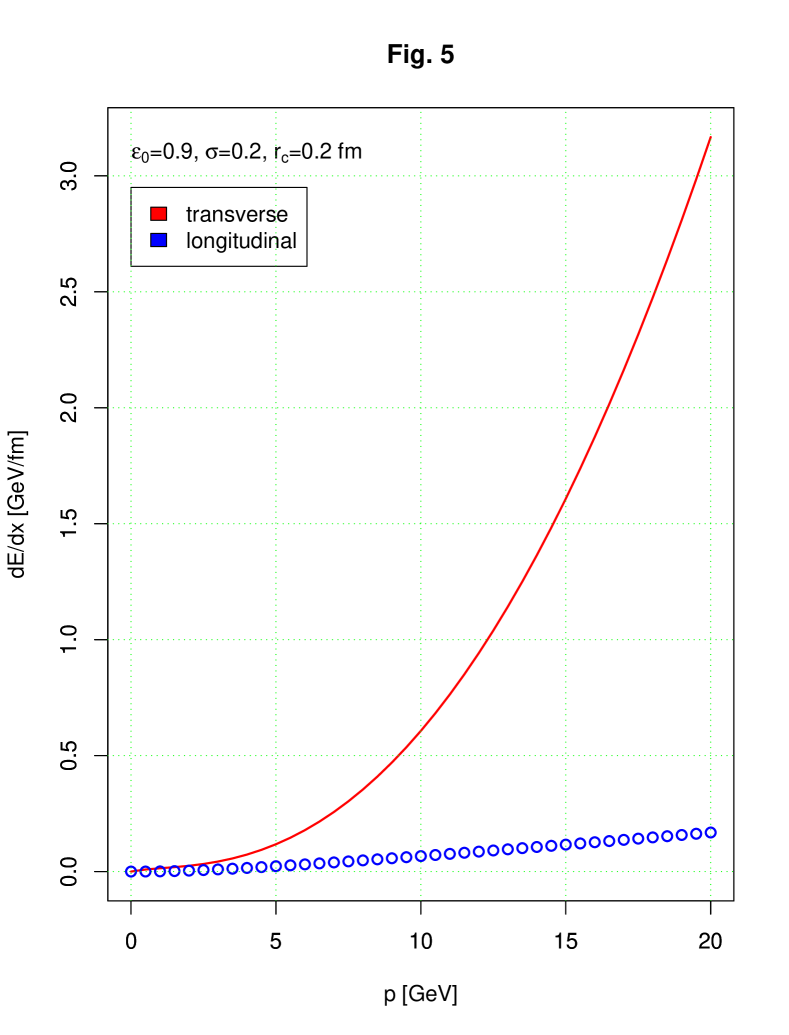
Figure 5: Energy dependence of quark transverse (red, solid) and longitudinal (blue, dotted) stochastic energy losses, $r_{c}=0.2\,{\rm fm}$, $\sigma=0.2$, $\varepsilon_{0}=0.9$.

To get a feeling on the magnitude of the stochastic energy loss in Gev/fm we plot it, for a quark with energy up to 20 GeV and parameter values $\alpha_{s}=0.2$, $r_{c}=0.2\,\,{\rm fm}$, $\sigma=0.2$ and $\varepsilon_{0}=0.9$, in Fig. 5. We see that at high energies the transverse stochastic loss can become quite substantial and exceed the values discussed in [6, 14].

Let us stress that the considered mechanism of stochastic quenching presents and additional source of energy loss with respect to mechanisms considered earlier in the literature. It is also important to have in mind that the above values constitute an order-of-magnitude estimate of stochastic quenching only since the above-described calculation is not reliable at $pr_{c}\gg 1$, also because of the strong dependence of the calculated energy loss on the cutoff $p$. Working out a consistent picture matching the above-described soft energy loss to the energy loss of hard modes requires developing a microscopic approach. This issue is a very important subject for future analysis. Another important task is to perform a quantitative analysis of the properties of inhomogeneous gluon medium created in ultrarelativistic nuclear collisions at LHC energies and use it as a basis for computing the stochastic energy losses of fast quarks and gluons. .

3 Conclusions

Stochastic energy loss of fast color particles in the random inhomogeneous medium was calculated to all orders in the fluctuation magnitude in the one-loop approximation. The dependence of stochastic losses on the bare chromodielectric permittivity $\varepsilon_{0}$, particle energy $p$ and fluctuation strength $\sigma$ was analyzed. The analysis has shown that stochastic energy loss can be of phenomenological importance. The strong dependence of the results on the value of ultraviolet cutoff indicates a necessity of developing a consistent microscopic approach allowing a unified treatment of energy losses due to soft and hard modes enabling a reliable quantitative calculation of the corresponding stochastic contribution. It is also of interest to consider in more details an interrelation between the above-considered mechanism of energy loss and effects of generic stochastic acceleration mechanism in random color fields considered in [16].

Acknowledgements

The authors are indebted to I.M. Dremin, S.M. Apenko, V.V. Losyakov and A.A. Rukhadze for useful discussions. We are also grateful to I.M. Dremin for reading the manuscript and suggesting improvements.

Appendix: Averaged vector field in statistically homogeneous medium.

To compute an expression for the disorder-averaged chromoelectric field determining the mean energy loss we have to write down a solution of the equation (2) for some given random profile $\xi({\bf r})$ and then average it over the Gaussian ensemble of random inhomogeneities with the two-point correlator (8). The first step is writing down an expression for the Green function ${\bf G}(w,{\bf r}|\,{\bf n},{\bf r}_{0})$ obeying the following equation:

$$\triangle{\bf G}-\nabla(\nabla{\bf G})+w^{2}{\bf G}=-w^{2}\xi({\bf r}){\bf G}+{\bf n}\delta({\bf r}-{\bf r_{0}})\,,$$ (13)

where ${\bf n}$ is a fixed unit three-vector and ${\bf r}_{0}$ is a fixed spatial point. In momentum space the equation (13) reads

$$\left[(w^{2}-{\bf k}^{2})\delta_{ij}+k_{i}k_{j}\right]G_{j}({\bf k})\,=\,-w^{2}(\hat{\xi}G_{i})({\bf k})+\frac{1}{(2\pi)^{3}}n_{i}{\rm e}^{-\imath{\bf k}{\bf r_{0}}}\,,$$ (14)

where

$$(\hat{\xi}{\mathbf{G}})({\mathbf{k}})=\frac{1}{(2\pi)^{3}}\int d^{3}{\bf r}d^{3}{\bf k^{\prime}}\xi({\mathbf{r}}){\mathbf{G}}({\bf k^{\prime}}){\rm e}^{\imath({\bf k^{\prime}}-{\mathbf{k}}){\bf r}}$$ (15)

Let us consider an iterative solution of (13):

$$G_{i}({w,\bf k}) = \frac{1}{(2\pi)^{3}}G^{0}_{ij}n_{j}{\rm e}^{-i{\bf k}{\bf r_{0}}}-\frac{1}{(2\pi)^{6}}w^{2}G^{0}_{ij_{1}}(\hat{\xi}A_{j_{1}j}n_{j}{\rm e}^{-\imath{\bf kr_{0}}})$$

$$+ \frac{1}{(2\pi)^{9}}w^{4}G^{0}_{ij_{1}}(\hat{\xi}G^{0}_{j_{1}j_{2}}(\hat{\xi}G^{0}_{j_{2}j}n_{j}{\rm e}^{-\imath{\bf kr_{0}}}))+\ldots\,,$$ (16)

where $G^{0}_{ij}(w,{\bf k})$ is a free propagator

$$G^{0}_{ij}=\frac{\delta_{ij}}{w^{2}-k^{2}}+\frac{k_{i}k_{j}}{w^{2}(k^{2}-w^{2})}$$

After averaging equation (Appendix: Averaged vector field in statistically homogeneous medium.) over the gaussian ensemble of fluctuations $\{\xi({\bf r})\}$ with the two-point correlator (8) we arrive at the algebraic Dyson equation for the averaged Green function $\langle G_{i}(w,{\bf k}|\,r_{c},\sigma,{\bf n})\rangle$:

$$\langle G_{i}\rangle=\frac{1}{(2\pi)^{3}}G^{0}_{ij}n_{j}{\rm e}^{-\imath{\bf k}{\bf r_{0}}}+G^{0}_{ik}\Pi_{kj}\langle G\rangle_{j}$$ (17)

so that

$$\langle{\bf G}(w,{\bf k}|\,r_{c},\sigma,{\bf n})\rangle=\frac{G^{0}(w,{\bf k})}{I-G^{0}(w,{\bf k})\Pi(w,{\bf k}|\,r_{c},\sigma)}\frac{{\bf n}}{(2\pi)^{3}}{\rm e}^{-\imath{\bf k}{\bf r_{0}}}$$ (18)

The averaged Green function (18) allows to compute the averaged chromoelectric field for an arbitrary external current $j^{a}({\bf r},t)$.

In the limit $\sigma^{2}(kr_{c})\ll 1$ one can keep the one-loop approximation for the polarization operator T$\Pi(w,{\bf k}|\,r_{c},\sigma)$:

$$\Pi_{ij}(w,{\bf k}|\,r_{c},\sigma)\approx w^{4}\int d^{3}k_{1}g(|\,{\bf k_{1}}-{\bf k}|,r_{c},\sigma)G^{0}_{ij}(w,{\bf k_{1}})$$ (19)

which can be computed analytically. Explicit expressions for its transverse and longitudinal components $\Pi^{t}_{ij}(w,{\bf k})$ and $\Pi^{l}_{ij}(w,{\bf k})$ take the form [15]:

$$\Pi^{t}(w,{\bf k}|\,r_{c},\sigma) = \sigma^{2}w^{2}\left[\frac{w^{2}}{(w+i\delta)^{2}-k^{2}}-\frac{\delta(\delta+iw)}{2k^{2}}\right.$$ (20)

$$+ \left.\frac{\delta^{2}+w^{2}+k^{2}}{k^{2}}\frac{\delta}{k}\arctan\left(\frac{ik}{w+i\delta}\right)\right]$$

and

$$\Pi^{l}(w,{\bf k}|\,r_{c},\sigma) = \sigma^{2}w^{2}\left[1+\frac{\delta(\delta+iw)}{2k^{2}}\right.$$ (21)

$$- \left.\frac{\delta^{2}+w^{2}+k^{2}}{k^{2}}\frac{\delta}{k}\arctan\left(\frac{ik}{w+i\delta}\right)\right]\,,$$

where $\delta=1/r_{c}$.

References

-
[1]
K. Adcox et al. [PHENIX Collaboration], Phys. Rev. Lett. 88 (2002), 022301
C. Adler et al. [STAR Collaboration], Phys. Rev. Lett. 89 (2002), 202301
C. Adler et al. [STAR Collaboration], Phys. Rev. Lett. 90 (2003), 082302
S.S. Adler et al. [PHENIX Collaboration], Phys. Rev. Lett. 91 (2003), 072301
J. Adams et al. [STAR Collaboration], Phys. Rev. Lett. 91 (2003), 172302 - [2] C. Alt et al. [NA49 Collaboration], Nucl. Phys. A774 (2006), 473
- [3] A. Kovner, U. Wiedemann, ”Gluon radiation and parton energy loss”, in Quark Gluon Plasma 3, Editors: R.C. Hwa and X.N. Wang, World Scientific, Singapore, 2003, 192; ArXiv: hep-ph/0304151.
- [4] M. Gyulassy, I. Vitev, X.-N. Wang, B.-W. Zhang, ”Jet quenching and radiative energy loss in dense nuclear matter”, in Quark Gluon Plasma 3, Editors: R.C. Hwa and X.N. Wang, World Scientific, Singapore, 2003, 123; ArXiv: nucl-th/0302077.
- [5] M. Gyulassy, D.H. Rischke, B. Zhang, Nucl. Phys. A613 (1997), 397
- [6] M. Gyulassy, M. Thoma, Nucl.Phys. B351 (1991), 491
- [7] S. Mrowczynski, Phys. Lett. B269 (1991), 383
- [8] L.D. Landau, E.M. Lifshitz, L.P. Pitaevski, ”Electrodynamics of continuous media”, Pergamon Press, Oxford, 1984
- [9] V.V. Tamoykin, Astrophysics and Space Science, 16 (1972), 120
- [10] I.M. Dremin, Int. J. Mod. Phys. A22 (2007) 3087; J. Phys. G35 (2008) 054001
- [11] I.M. Dremin, M.R. Kirakosyan, A.V. Leonidov, A.V. Vinogradov, ”Cherenkov Glue in Opaque Nuclear Medium”, arXiv:0809.2472 [hep-ph]
- [12] S.P. Kapitsa, ZHETP 39 (1960), 1367
- [13] Yu.N. Barabanenkov, Yu.A. Kravtsov, S.M. Rytov, V.I. Tatarsky, UFN 102 (1970), 3 (in Russian)
- [14] J.D. Bjorken, Energy Loss of Energetic Partons in Quark-Gluon Plasma: Possible Extinction of High Jets in Hadron-Hadron Collisions, preprint FERMILAB-Pub-82/59-THY
- [15] M.R. Kirakosyan, A.V. Leonidov, ”Energy Loss in Stochastic Abelian Medium”, arXiv:0809.2179 [hep-ph]
- [16] A. Leonidov, Zeit. Phys. C66 (1995), 263