On Gravitational Waves in Spacetimes with a
Nonvanishing Cosmological Constant

Abstract

We study the effect of a cosmological constant $\Lambda$ on the propagation and detection of gravitational waves. To this purpose we investigate the linearised Einstein’s equations with terms up to linear order in $\Lambda$ in a de Sitter and an anti–de Sitter background spacetime. In this framework the cosmological term does not induce changes in the polarization states of the waves, whereas the amplitude gets modified with terms depending on $\Lambda$. Moreover, if a source emits a periodic waveform, its periodicity as measured by a distant observer gets modified. These effects are, however, extremely tiny and thus well below the detectability by some twenty orders of magnitude within present gravitational wave detectors such as LIGO or future planned ones such as LISA.

I Introduction

The discovery that the expansion of the Universe is accelerating Peebles and Ratra (2003), which can be interpreted as due to a cosmological constant $\Lambda$, has triggered a lot of recent works with the aim to study how $\Lambda$ affects e. g. celestial mechanics and the motion of massive bodies. In principle the cosmological constant should take part in phenomena on every physical scale. For instance, it has been studied which limits on $\Lambda$ can be put from solar system measurements, such as the effect on the perihelion precession of the solar systemplanets Islam (1983); Wright (1998); Kerr et al. (2003); Jetzer and Sereno (2006); Sereno and Jetzer (2006, 2007); Iorio (2006). The cosmological constant could also influence gravitationallensing Rindler and Ishak (2007); Sereno (2008) and play a role in the gravitational equilibrium of large astrophysical structures Balaguera-Antolínez and Nowakowski (2005). A natural question which arises is how the cosmological term affects gravitational waves. Clearly, we expect such an effect to be very tiny, nonetheless we believe that it is worthwhile to investigate it given the ongoing efforts in upgrading or building gravitational wave observatories either Earth bounded or in space.

In this paper we study gravitational waves in spacetimes with a nonvanishing cosmological constant $\Lambda$ in the framework of perturbation theory with respect to de Sitter (dS) and anti–de Sitter (AdS) metrics. There are few articles in the literature devoted to the question on how the cosmological constant affects gravitational waves. Some approaches consider exact solutions of the Einstein’s equations with a cosmological term relying on the Kundt class of spacetimes, which admit a non-twisting and expansion–free null vectorfield Ozsváth et al. (1985); Bičák and Podolský (1999a, b). In Bičák and Podolský (1999a, b) these spacetimes are interpreted as plane gravitational waves with polarizations “$+$” and “$\times$” which propagate on dS and AdS backgrounds.

A perturbative approach different from ours can be found in Lu (1988), where the Einstein equations with a cosmological term are linearised with respect to a Minkowski background metric. By choosing a particular non Hilbert gauge this leads then to a Klein–Gordon equation and thus to a nontrivial dispersion relation.

Furthermore, we refer to some works on the scalar wave equation in dS and Schwarzschild-dS spacetimes Polarski (1989); Dafermos and Rodnianski (2007); Yagdjian and Galstian (2007); Bony and Hafner (2007). These treatments are, however, not directly connected to the present work, since the equations resulting from the linearisation of Einstein’s equations are coupled partial differential equations for six independent variables.

The outline of the paper is as follows: in Section II we derive the linearised Einstein equations with respect to a dS or AdS background, which are represented by some generalized Klein–Gordon equations. Since a closed exact solution is not evident, we examine in Section III a perturbation expansion of these equations up to linear order with respect to $\Lambda$. In Section IV we calculate the corresponding first order contributions to the amplitudes. The effects on directly measurable quantities are discussed in Section V.

For the details of the linearisation of the Einstein equations with respect to an arbitrary differentiable background metric we refer e. g. to the textbooks Straumann (2004); Landau and Lifshitz (1992) or the review Flanagan and Hughes (2005).

As far as notation is concerned: Greek letters denote spacetime indices and range from $0$ to $3$, whereas Latin letters denote space indices and range from $1$ to $3$. If not stated otherwise, we use geometrical units ($c=1$ and $G=1$).

II Linearised Einstein’s Equations with Cosmological Term

Let $(M,g_{\mu\nu})$ be a 4-dimensional Lorentz manifold with metric $g_{\mu\nu}$ of signature $(+,-,-,-)$. Let $R_{\mu\nu}$, resp. $R$, denote the Ricci tensor, resp. scalar, of $g_{\mu\nu}$. Then the vacuum Einstein equations with cosmological term read

$$R_{\mu\nu}-\left(\frac{R}{2}-\Lambda\right)g_{\mu\nu}=0.$$ (1)

In what follows we consider a perturbed metric

$$g_{\mu\nu}=\tilde{g}_{\mu\nu}+h_{\mu\nu},$$ (2)

where $\tilde{g}_{\mu\nu}$ is a static background metric and $h_{\mu\nu}$ is a non–static perturbation with $|h_{\mu\nu}|\ll|\tilde{g}_{\mu\nu}|$. Up to first order in $h$ the indices are uppered and lowered by $\tilde{g}_{\mu\nu}$. Indicating the unperturbed Riemann tensor by $\tilde{R}_{\mu\nu\lambda\rho}$ and consequently the Ricci tensor, resp. scalar, by $\tilde{R}_{\mu\nu}=\tilde{R}^{\lambda}_{\phantom{\lambda}\mu\nu\lambda}$, resp. $\tilde{R}=\tilde{R}^{\lambda}_{\phantom{\lambda}\lambda}$, we can write the expansion of equation (1) up to linear order in $h_{\mu\nu}$ as

$$\tilde{R}_{\mu\nu} + R_{\mu\nu}(h)-\left(\frac{\tilde{R}}{2}+\frac{R(h)}{2}-\Lambda\right)\tilde{g}_{\mu\nu}$$

$$- \left(\frac{\tilde{R}}{2}-\Lambda\right)h_{\mu\nu}+\mathcal{O}(h^{2})=0,$$

where the linear contributions to the Ricci tensor Straumann (2004) and Ricci scalar are

$$R_{\mu\nu}(h) = \frac{1}{2}\Big{(}h^{\lambda}_{\phantom{\lambda}\mu;\nu;\lambda}+h^{\lambda}_{\phantom{\lambda}\nu;\mu;\lambda}$$

$$-h^{\phantom{\mu\nu};\lambda}_{\mu\nu\phantom{;\lambda};\lambda}-h^{\lambda}_{\phantom{\lambda}\lambda;\mu;\nu}\Big{)},$$

$$R(h) = R^{\lambda}_{\phantom{\lambda}\lambda}(h)-h^{\lambda\rho}\tilde{R}_{\lambda\rho}.$$

The semicolon denotes the covariant derivative with respect to $\tilde{g}_{\mu\nu}$. The terms in (II) which are independent of $h_{\mu\nu}$ satisfy equation (1) with $\tilde{g}_{\mu\nu}$,

$$\tilde{R}_{\mu\nu}-\left(\frac{\tilde{R}}{2}-\Lambda\right)\tilde{g}_{\mu\nu}=0.$$ (5)

The terms linear in $h_{\mu\nu}$ are determined by

$$R_{\mu\nu}(h)-\frac{R(h)}{2}\tilde{g}_{\mu\nu}-\left(\frac{\tilde{R}}{2}-\Lambda\right)h_{\mu\nu}=0.$$ (6)

In order to see explicitly the Klein–Gordon character of (6), we rewrite this equation using the expressions in equation (II) and the trace-reversed quantity $\tilde{\gamma}_{\mu\nu}:=h_{\mu\nu}-\frac{h}{2}\tilde{g}_{\mu\nu}$, $h:=h^{\lambda}_{\phantom{\lambda}\lambda}$. We are then left with

$$\tilde{\gamma}^{\phantom{\mu\nu};\lambda}_{\mu\nu\phantom{;\lambda};\lambda} + \tilde{\gamma}^{\phantom{\lambda\mu};\lambda}_{\lambda\mu\phantom{\lambda};\nu}+\tilde{\gamma}^{\phantom{\lambda\nu};\lambda}_{\lambda\nu\phantom{\lambda};\mu}$$

$$+ 2\tilde{R}_{\lambda\mu\rho\nu}\tilde{\gamma}^{\lambda\rho}-\tilde{R}_{\lambda\mu}\tilde{\gamma}^{\phantom{\nu}\lambda}_{\nu}-\tilde{R}_{\lambda\nu}\tilde{\gamma}^{\phantom{\mu}\lambda}_{\mu}$$

$$- \tilde{R}_{\lambda\rho}\tilde{g}_{\mu\nu}\left(\tilde{\gamma}^{\lambda\rho}-\frac{\tilde{\gamma}^{\sigma}_{\phantom{\sigma}\sigma}}{2}\tilde{g}^{\lambda\rho}\right)$$

$$+ 2\Lambda\left(\tilde{\gamma}_{\mu\nu}-\frac{\tilde{\gamma}^{\lambda}_{\phantom{\lambda}\lambda}}{2}\tilde{g}_{\mu\nu}\right)=0,$$

In contrast to the corresponding result for the Einstein’s equations without cosmological term (where instead of eq.(6) we have $R_{\mu\nu}(h)=0$ Straumann (2004)), the equations (II) feature in addition the two last terms.

In order to analyse further the equations (5) and (II) we fix the background as follows. It is well known that a dS resp. AdS metric solves the equations (1) exactly. For our purposes it is thus the natural choice for the background. We note that at this point a Schwarzschild–de Sitter solution might have been chosen as well. We avoid this since we are interested in a region of spacetime which is far from sources of gravitational radiation. We now choose an appropriate coordinate system for the background spacetime $(M,\tilde{g}_{\mu\nu})$. Let $p:I\subset\mathbb{R}\to M$ be the locus of an observer at rest Straumann (2004) and let $\phi:M\to\mathbb{R}^{4}$, $m\mapsto(t,x,y,z)$ be a coordinate chart such that $\phi(p(t))=(t,0,0,0)$. An exact solution of (5) in the chart $\phi$ is given by

$$\tilde{g}_{00} = \left(\frac{1-\frac{\Lambda}{12}r^{2}}{1+\frac{\Lambda}{12}r^{2}}\right)^{2},$$ (8)

$$\tilde{g}_{ii} = \frac{-1}{\left(1+\frac{\Lambda}{12}r^{2}\right)^{2}},$$

$$\tilde{g}_{ij} = 0,\quad i\neq j,$$

where $r:=\sqrt{x^{2}+y^{2}+z^{2}}$. The solution (8) is valid inside the null horizon $r^{2}=12/|\Lambda|$, which depends on the choice of the observer $p$. The apparent spacelike nature of the normal to this surface is due to the use of isotropic coordinates. For later use we denote the corresponding hypersurface in our coordinate chart by $\Omega:=\{(x,y,z)\in\mathbb{R}^{3}\ |\ r^{2}<12/|\Lambda|\}$. However, for the following applications it suffices to consider a region which is much smaller than $\Omega$. The metric (8) was first introduced in de Sitter (1917) and is therefore known as dS resp. AdS metric according to $\Lambda>0$ resp. $\Lambda<0$. Its Riemann tensor is given by

$$\tilde{R}_{\mu\nu\lambda\rho}=\frac{\Lambda}{3}\left(\tilde{g}_{\mu\lambda}\tilde{g}_{\nu\rho}-\tilde{g}_{\mu\rho}\tilde{g}_{\nu\lambda}\right).$$ (9)

The equations (II) form a family of ten coupled generalised Klein–Gordon equations for which an algorithm providing closed solutions is not known. We point out that the high symmetry of dS resp. AdS allows to derive exact solutions of equation (1) Bičák and Podolský (1999a, b). Moreover, if we impose the Hilbert gauge condition $\tilde{\gamma}^{\phantom{\mu\nu};\nu}_{\mu\nu}=0$, then the trace of equation (II) turns into a simple Klein–Gordon equation for the trace of $\tilde{\gamma}_{\mu\nu}$ on dS resp. AdS space,

$$\tilde{\gamma}_{\phantom{\lambda};\lambda}^{;\lambda}+2\Lambda\tilde{\gamma}=0,$$ (10)

which may be solved exactly by using separation of variables Polarski (1989). However, since we are interested in the physical consequences of the cosmological constant for all the components $\tilde{\gamma}_{\mu\nu}$ (and not just for the trace) in the regime of a metric perturbation, equation (10) does not provide enough information. Moreover, the perturbed solutions derived below are traceless, thus only the trivial solution of (10) is relevant for our purposes.

Note that the contraction of the equations (II) with the stationary Killing field $(\partial_{t})^{\lambda}$ might lead to simpler equations. However, the resulting equations are still non–scalar, as this is suggested by the equations (22) below. Thus the derivation of an analytic result, if possible, would be quite involved.

Although it would be useful to supplement the perturbative calculation below with analytic results in order to gain more confidence in the former, it seems that the effort for such a program would exceed the derivation of the perturbative results and definitely goes beyond the scope of the present work. We therefore content ourselves with an expansion of (II) with respect to $\Lambda$ up to linear order.

We remark that such an expansion with respect to $\Lambda$ is consistent with the expansion with respect to $h_{\mu\nu}$. Equations (5) may also be expanded with respect to $\Lambda$, and the coefficients of each order fulfill the equations subsequently. This point of view would correspond to a one–parameter perturbation of the Minkowski metric $\eta_{\mu\nu}={\rm diag}\left(1,-1,-1,-1\right)$ of the form

$$g_{\mu\nu}=\eta_{\mu\nu}+\sum_{n=1}^{\infty}\Lambda^{n}h^{(n)}_{\mu\nu}.$$ (11)

Each coefficient $h^{(n)}_{\mu\nu}$ could be written as

$$h^{(n)}_{\mu\nu}=\tilde{h}^{(n)}_{\mu\nu}+\bar{h}^{(n)}_{\mu\nu},$$ (12)

where

$$\sum_{n=1}^{\infty}\Lambda^{n}\tilde{h}^{(n)}_{\mu\nu}=\tilde{g}_{\mu\nu}-\eta_{\mu\nu}\quad\textrm{and}\quad\sum_{n=1}^{\infty}\Lambda^{n}\bar{h}^{(n)}_{\mu\nu}=h_{\mu\nu}.$$ (13)

In other words, the $\tilde{h}^{(n)}_{\mu\nu}$ contain the contributions from the background, whereas the $\bar{h}^{(n)}_{\mu\nu}$ describe the waveform. Since $\Lambda$ carries the physical unit of $(\mathrm{Length})^{-2}$, the $n^{\mathrm{th}}$ order coefficients of the expansions above carry the physical unit $(\mathrm{Length})^{2n}$.

III Approximate Solution of the Linearised Equations

In particular the perturbation expansion with respect to $\Lambda$ is based on the assumption $r\ll\sqrt{12/|\Lambda|}$. We collect terms proportional to $\Lambda^{n}$ and denote them by $\mathcal{O}(\Lambda^{n})$. For $r\ll\sqrt{12/|\Lambda|}$ equation (8) yields

$$\tilde{g}_{\mu\nu}=\eta_{\mu\nu}+\mathcal{O}(\Lambda).$$ (14)

Then the connection coefficients are of order $\mathcal{O}(\Lambda)$ and so are $\tilde{R}_{\mu\nu\lambda\rho}$ and $\tilde{R}_{\mu\nu}$ by (9), such that equation (II) may be written as

$$\gamma^{\phantom{\mu\nu},\lambda}_{\mu\nu\phantom{,\lambda},\lambda}+\gamma^{\phantom{\lambda\mu},\lambda}_{\lambda\mu\phantom{\lambda},\nu}+\gamma^{\phantom{\lambda\nu},\lambda}_{\lambda\nu\phantom{\lambda},\mu}+\Lambda D_{\mu\nu}(\gamma)+\mathcal{O}(\Lambda^{2})=0,$$ (15)

where $\gamma_{\mu\nu}:=h_{\mu\nu}-\frac{h}{2}\eta_{\mu\nu}$, the comma denotes partial derivatives, the indices are uppered and lowered by $\eta_{\mu\nu}$, and $D_{\mu\nu}$ is a linear hyperbolic differential operator of second order. We are thus led to consider the variable $\gamma_{\mu\nu}$ instead of $\tilde{\gamma}_{\mu\nu}$. These variables differ if the trace $h$ does notvanish. However, the solutions which are considered in the following sections are trace–free, and therefore they satisfy $\tilde{\gamma}_{\mu\nu}=\gamma_{\mu\nu}=h_{\mu\nu}$.

Hereafter we will neglect the terms of order $\mathcal{O}(\Lambda^{2})$. Then $\Lambda$ lends itself as expansion parameter for the following perturbation procedure.

Let $\square:=\partial^{\lambda}\partial_{\lambda}$ denote the d’Alembert operator. We assume that the exact solution of the operator equation

$$\square\gamma_{\mu\nu}+\gamma^{\phantom{\lambda\mu},\lambda}_{\lambda\mu\phantom{\lambda},\nu}+\gamma^{\phantom{\lambda\nu},\lambda}_{\lambda\nu\phantom{\lambda},\mu}+\Lambda D_{\mu\nu}(\gamma)=0$$ (16)

can be written as a power series in $\Lambda$. Up to linear order we then have

$$\gamma_{\mu\nu}=\gamma_{\mu\nu}^{(0)}+\Lambda\gamma_{\mu\nu}^{(1)}+\mathcal{O}(\Lambda^{2}),$$ (17)

where the coefficients $\gamma_{\mu\nu}^{(1)}$ carry the physical unit $(\mathrm{Length})^{2}$. Thus a comparison to the case of a vanishing cosmological constant is achieved simply by considering only the zeroth order terms. Plugging (17) into (16) yields by comparing coefficients order by order

$$\square\gamma_{\mu\nu}^{(0)}+\gamma^{(0)\phantom{,},\lambda}_{\lambda\mu\phantom{\lambda,},\nu}+\gamma^{(0)\phantom{,},\lambda}_{\lambda\nu\phantom{\lambda,},\mu} = 0,$$ (18)

$$\square\gamma_{\mu\nu}^{(1)} = -D_{\mu\nu}(\gamma^{(0)}).$$

On the first equation in (18) we impose the hilbert gauge condition $\gamma^{\phantom{\mu\nu},\nu}_{\mu\nu\phantom{\nu}}=0$ and afterwards choose the transverse traceless gauge. Thus the fundamental solutions are plane gravitational waves with the two linear polarization states “$+$” and “$\times$”.The solutions of the second equation in (18) are then determined by the expression

$$\gamma_{\mu\nu}^{(1)}=-\mathcal{G}*D_{\mu\nu}(\gamma^{(0)}),$$ (19)

where

$$\mathcal{G}(t,r)=\frac{\delta(t-r)\theta(t)}{4\pi r}$$ (20)

is the Green’s function of the d’Alembert operator and the star denotes the convolution. The domain of integration in (19) is $\mathbb{R}^{3}$, which may be interpreted as lowest order approximation of $\Omega$. In order to avoid divergences we need to choose an appropriate decrease for the amplitude of $\gamma_{\mu\nu}^{(0)}$ for $r\to\infty$. For our case a power counting argument requires the asymptotic behaviour $\left|\gamma_{\mu\nu}^{(0)}\right|\sim r^{-\alpha}$ for $\alpha>2$. Accordingly one requires the boundary conditions

$$\lim_{r\to\infty}\gamma_{\mu\nu}^{(1)}=0\qquad\textrm{and}\qquad\lim_{r\to\infty}\gamma^{(1)}_{\mu\nu,\lambda}=0.$$ (21)

However, in the following sections we will consider only a small region of spacetime, so that the question of the behaviour for $r\to\infty$ is not essential. We will, therefore, assume that the intersection of any spacelike hypersurface with the support of $\gamma_{\mu\nu}^{(0)}$ and thus the domain of integration in (19) is compact.

It is understood that in contrast to Minkowski space the notion of planarity of a wavefront has to be modified for waves in curved spacetime. In the framework of exact solutions of the Einstein’s equations this is achieved by demanding that the spacetime admits a null vectorfield which is non-twisting and expansion-free.

However, in the perturbative approach we naturally assume that the wave front is a hyperplane up to lowest order. In a consistent perturbation expansion we are thus advised to assume that the fundamental solutions $\gamma^{(0)}_{\mu\nu}$ of the first equation in (18) is a Minkowski–plane wave. As mentioned above we restrict the support of $\gamma^{(0)}_{\mu\nu}$. In doing so we need to avoid further destruction of the symmetries of plane waves. Therefore we choose the domain of integration in (19) to be spherically symmetric and indicate it by $\Omega_{\mathcal{R}}:=\{(x,y,z)\in\mathbb{R}^{3}\ |\ r<\mathcal{R}\}$.

IV Plane Wave Propagation

We now choose the coordinate chart $\phi$ such that $\gamma^{(0)}_{\mu\nu}$ is a plane transverse traceless solution and the non–vanishing components are $\gamma^{(0)}_{11}$, $\gamma^{(0)}_{22}=-\gamma^{(0)}_{11}$ and $\gamma^{(0)}_{12}$. These components are functions of the retarded time $z-t$ and describe thus a plane wave propagating in $z$–direction. The non–vanishing components of $D_{\mu\nu}(\gamma^{(0)})$ are then given by

$$D_{01}(\gamma^{(0)}) = \frac{7}{6}\left(x\partial_{t}\gamma^{(0)}_{11}+y\partial_{t}\gamma^{(0)}_{12}\right),$$ (22)

$$D_{02}(\gamma^{(0)}) = \frac{7}{6}\left(x\partial_{t}\gamma^{(0)}_{12}-y\partial_{t}\gamma^{(0)}_{11}\right),$$

$$D_{11}(\gamma^{(0)}) = \frac{r^{2}}{6}\left(2\partial_{tt}\gamma^{(0)}_{11}-\partial_{zz}\gamma^{(0)}_{11}\right)$$

$$-\frac{z}{6}\partial_{z}\gamma^{(0)}_{11}+\frac{2}{3}\gamma^{(0)}_{11},$$

$$D_{22}(\gamma^{(0)}) = -D_{11}(\gamma^{(0)}),$$

$$D_{12}(\gamma^{(0)}) = \frac{r^{2}}{6}\left(2\partial_{tt}\gamma^{(0)}_{12}-\partial_{zz}\gamma^{(0)}_{12}\right)$$

$$-\frac{z}{6}\partial_{z}\gamma^{(0)}_{12}+\frac{2}{3}\gamma^{(0)}_{12},$$

$$D_{13}(\gamma^{(0)}) = \frac{5}{6}\left(x\partial_{z}\gamma^{(0)}_{11}+y\partial_{z}\gamma^{(0)}_{12}\right),$$

$$D_{23}(\gamma^{(0)}) = \frac{5}{6}\left(x\partial_{z}\gamma^{(0)}_{12}-y\partial_{z}\gamma^{(0)}_{11}\right),$$

We now restrict ourselves to the investigation of the contributions to the “$+$”–mode of $\gamma^{(0)}$. An analogous result may be derived for the “$\times$”–mode. We have $\gamma^{(0)}_{11}=f(z-t)$ and $\gamma^{(0)}_{12}=0$, where $f:D\subset\mathbb{R}\to\mathbb{R}$ is an arbitrary smooth function. Equations (22) yield

$$D_{01}(\gamma^{(0)}) = -\frac{7x}{6}f^{\prime}(z-t),$$ (23)

$$D_{02}(\gamma^{(0)}) = \frac{7y}{6}f^{\prime}(z-t),$$

$$D_{11}(\gamma^{(0)}) = \frac{r^{2}}{6}f^{\prime\prime}(z-t)-\frac{z}{6}f^{\prime}(z-t)+\frac{2}{3}f(z-t),$$

$$D_{22}(\gamma^{(0)}) = -D_{11}(\gamma^{(0)}),$$

$$D_{12}(\gamma^{(0)}) = 0,$$

$$D_{13}(\gamma^{(0)}) = \frac{5x}{6}f^{\prime}(z-t),$$

$$D_{23}(\gamma^{(0)}) = -\frac{5y}{6}f^{\prime}(z-t).$$

Thus we are able to calculate the first order corrections by using formula (19), i. e.

$$\gamma^{(1)}_{\mu\nu}(t,\vec{x})=-\frac{1}{4\pi}\int_{\Omega_{\mathcal{R}}}\frac{D_{\mu\nu}(\gamma^{(0)})\left(t-|\vec{x}-\vec{\xi}|,\vec{\xi}\right)}{|\vec{x}-\vec{\xi}|}\,d^{3}\xi.$$ (24)

In particular, all components vanish except

$$\gamma^{(1)}_{11}(t,\vec{x}) = \frac{1}{24\pi}\int_{\Omega_{\mathcal{R}}}\Bigg{[}(\vec{\xi})^{2}f^{\prime\prime}\left(\xi_{3}-(t-|\vec{x}-\vec{\xi}|)\right)$$

$$-\xi_{3}f^{\prime}\left(\xi_{3}-(t-|\vec{x}-\vec{\xi}|)\right)$$

$$+4f\left(\xi_{3}-(t-|\vec{x}-\vec{\xi}|)\right)\Bigg{]}\frac{d^{3}\xi}{|\vec{x}-\vec{\xi}|}$$

$$\gamma^{(1)}_{22}(t,\vec{x}) = -\gamma^{(1)}_{11}(t,\vec{x}).$$

This result indicates that in contrast to the amplitude the polarization remains unchanged up to this order, thus preserving the quadrupole character of gravitational radiation. Though an evaluation of the equation (IV) in general can hardly be carried out analytically for arbitrary events $(t,\vec{x})$, it still may be computed along the locus $p(t)$ of the observer using spherical coordinates. We now introduce physical units. Let $\gamma_{11}(t,\vec{0})=f(\omega t)$, where $\omega$ denotes a frequency, and let $c$ denote the speed of light. Then the non–vanishing components of the perturbation $h_{\mu\nu}$ in (2) are determined by

$$h_{11}(t,\vec{0}) = \gamma_{11}(t,\vec{0})\approx\left(\gamma^{(0)}_{11}+\Lambda\gamma^{(1)}_{11}\right)(t,\vec{0})$$

$$= f(\omega t)+\frac{\Lambda}{24\pi}\Bigg{[}\frac{\mathcal{R}^{3}\omega}{3c}f^{\prime}(-\omega t)$$

$$+\frac{\mathcal{R}^{2}}{2}\left(f(-\omega t)-f\left(\frac{2\mathcal{R}\omega}{c}-\omega t\right)\right)$$

$$-\frac{\mathcal{R}c}{\omega}\left(5f^{\uparrow}(-\omega t)-f^{\uparrow}\left(\frac{2\mathcal{R}\omega}{c}-\omega t\right)\right)$$

$$-\frac{2c^{2}}{\omega^{2}}\left(f^{\uparrow\uparrow}(-\omega t)-f^{\uparrow\uparrow}\left(\frac{2\mathcal{R}\omega}{c}-\omega t\right)\right)\Bigg{]},$$

where we have denoted the primitive of any function $g:D\subset\mathbb{R}\to\mathbb{R}$ by

$$g^{\uparrow}(t):=\int^{t}g(t^{\prime})dt^{\prime}.$$ (27)

Due to the parameter $\mathcal{R}$, the formula (IV) is not yet in a form which allows an immediate meaningful physical interpretation. A priori $\mathcal{R}$ is a positive real number which measures the dimension of the support of $\gamma^{(0)}_{\mu\nu}$ in Minkowski spacetime. A posteriori we gather from equation (IV) that the perturbation expansion is reasonable if

$$\lim_{\Lambda\to 0}\frac{\Lambda\mathcal{R}^{3}\omega}{c}=\lim_{\Lambda\to 0}\Lambda\mathcal{R}^{2}=\lim_{\Lambda\to 0}\frac{\Lambda\mathcal{R}c}{\omega}=\lim_{\Lambda\to 0}\frac{\Lambda c^{2}}{\omega^{2}}=0.$$ (28)

Thus we formally obtain $\Lambda$–dependent constraints on $\mathcal{R}$ and $\omega$. If we impose the the geometrical optics limit, $\mathcal{R}\gg c/\omega$, we have

$$\frac{\mathcal{R}^{3}\omega}{c}\gg\mathcal{R}^{2}\gg\frac{\mathcal{R}c}{\omega}\gg\frac{c^{2}}{\omega^{2}},$$ (29)

so that all the limites in (28) follow from the first one. In Section V we give more comments on the interpretation of $\mathcal{R}$. In particular we find that for our purposes we can assume $\mathcal{R}\ll 1/\sqrt{|\Lambda|}$. Since $\omega$ is a constant parameter, the limits in (28) are fullfilled. The condition $\left|\Lambda\gamma^{(1)}_{11}\right|\ll\left|\gamma^{(0)}_{11}\right|$ yields then $\Lambda\mathcal{R}^{3}\omega/c\ll 1$, which gives an upper bound on $\omega$.

As an illustration of the above results we consider the example $f(\omega t):=\sin(\omega t)$. Due to the conditions in equation (29) we can neglect the terms with coefficients proportional to $c^{2}/\omega^{2}$, $\mathcal{R}c/\omega$ and $\mathcal{R}^{2}$, so that to leading order we get

$$h_{11}(t,\vec{0}) \approx \sin(\omega t)+\frac{\Lambda\mathcal{R}^{3}\omega}{72\pi c}\cos(\omega t).$$ (30)

Since $\Lambda\mathcal{R}^{3}\omega/c\ll 1$, this can also be written as

$$h_{11}(t,\vec{0}) \approx \sin\left(\omega\left(t+\frac{\Lambda\mathcal{R}^{3}}{72\pi c}\right)\right).$$ (31)

For a periodic $\gamma^{(0)}_{\mu\nu}$, equation (30) shows that the correction $\gamma^{(1)}_{\mu\nu}$ features a modified amplitude, whereas (31) yields a modification of the frequency. In the following section we show that $\mathcal{R}$ depends on the proper time of the observer. In general the frequency therefore changes with varying time.

V Effects on Measurable Quantities

The coordinate data in the in this section corresponds to the lowest order approximation of the chart $\phi$, which represents a Minkowski background. Consider a source which starts to emit gravitational radiation at some event $(-t_{0},\vec{x}_{0})$ so that an observer at large distance $|\vec{x}_{0}|=t_{0}$ would start to perceive an approximately plane wave at the event $(0,\vec{0})$. Assume that the wave at this event had the shape of the function $f$ up to lowest order. Let the observer at $p(t)$ carry out a measurement during a time interval $[0,\tau]$, such that $\tau\ll t_{0}$. In addition to the wave $f$, the observer would measure increasing retarded contributions $\gamma^{(1)}_{\mu\nu}$ with increasing $\tau$. These contributions originate from a spherical region within $r\leq\tau$. For the present measurement we thus have $\mathcal{R}=\tau$. Reasonably we have $\tau\ll 1/\sqrt{|\Lambda|}$ and therefore $\mathcal{R}\ll 1/\sqrt{|\Lambda|}$. Using again physical units, for $\Lambda\approx 10^{-52}\mathrm{m}^{-2}$ this yields

$$\tau\ll 10^{18}\mathrm{s}\approx 10^{11}\mathrm{yr}.$$ (32)

Let $\tau_{\mathrm{yr}}$ denote the length of the measurement in years, and let $c\approx 3\cdot 10^{8}\mathrm{m}/\mathrm{s}$. Then the condition

$$\Lambda c^{2}\tau^{3}\omega\ll 1$$ (33)

and the geometrical optics limit $\tau\gg 1/\omega$ yield the following constraints on $\omega$:

$$\frac{1}{\tau_{\mathrm{yr}}}\cdot 10^{-7}\mathrm{Hz}\ll\omega\ll\frac{1}{\tau_{\mathrm{yr}}^{3}}\cdot 10^{15}\mathrm{Hz}.$$ (34)

The condition (32) implies a non–vanishing range for the parameter $\omega$ in (34). For $\tau$ ranging from a couple of minutes up to several thousands of years, the radiation emitted by typical sources of gravitational waves features frequencies in this range.

The measurement via the equation for geodesic deviation is carried out analogously to the case $\Lambda=0$ (cf. Straumann (2004), e. g.). We have

$$\frac{d^{2}n^{i}}{dt^{2}}=-R^{i}_{\phantom{i}00j}n^{j},$$ (35)

where $\vec{n}=(n^{1},n^{2},n^{3})$ is the separation vector between two neighbouring members of a congruence of timelike geodesics Straumann (2004). We expand the Riemann tensor with respect to the perturbation $h_{\mu\nu}$:

$$R_{\mu\nu\lambda\rho}=\tilde{R}_{\mu\nu\lambda\rho}+R_{\mu\nu\lambda\rho}(h)+\mathcal{O}(h^{2}),$$ (36)

where the linear contribution to the Riemann tensor is given by Landau and Lifshitz (1992)

$$R^{\mu}_{\phantom{\mu}\nu\lambda\rho}(h) = \frac{1}{2}\Big{(}h^{\mu}_{\phantom{\mu}\nu;\rho;\lambda}+h^{\mu}_{\phantom{\mu}\rho;\nu;\lambda}-h^{\phantom{\nu\rho};\mu}_{\nu\rho\phantom{;\mu};\lambda}$$

$$-h^{\mu}_{\phantom{\mu}\nu;\lambda;\rho}-h^{\mu}_{\phantom{\mu}\lambda;\nu;\rho}+h^{\phantom{\nu\lambda};\mu}_{\nu\lambda\phantom{;\mu};\rho}\Big{)}.$$

For any measurement it is always possible to configure the detector such that it is sensitive only to the “$+$”–mode of the wave Flanagan and Hughes (2005). We assume that this is the case in the following paragraphs. Therefore, in the present case we consider only the following components of $R_{\mu\nu\lambda\rho}$:

$$\tilde{R}^{i}_{\phantom{i}00j} = -\frac{\Lambda}{3}\delta^{i}_{j}+\mathcal{O}(\Lambda^{2})$$ (38)

$$R^{1}_{\phantom{1}001}(h) = -\frac{1}{2}\left(\partial_{tt}\gamma^{(0)}_{11}+\Lambda\left(\partial_{tt}\gamma^{(1)}_{11}+\frac{1}{3}\vec{x}\cdot\nabla\gamma^{(0)}_{11}\right)\right)$$

$$+\mathcal{O}(\Lambda^{2})=-R^{2}_{\phantom{2}002}(h).$$

Along the locus of $p(t)$ the components of equation (35) thus read

$$\frac{d^{2}n^{1}}{dt^{2}} = \left[\frac{1}{2}\frac{d^{2}\gamma^{(0)}_{11}}{dt^{2}}+\Lambda\left(\frac{1}{3}+\frac{1}{2}\frac{d^{2}\gamma^{(1)}_{11}}{dt^{2}}\right)\right]n^{1},$$ (39)

$$\frac{d^{2}n^{2}}{dt^{2}} = \left[-\frac{1}{2}\frac{d^{2}\gamma^{(0)}_{11}}{dt^{2}}+\Lambda\left(\frac{1}{3}-\frac{1}{2}\frac{d^{2}\gamma^{(1)}_{11}}{dt^{2}}\right)\right]n^{2},$$

$$\frac{d^{2}n^{3}}{dt^{2}} = \frac{\Lambda}{3}n^{3}.$$

Let $n^{i}(t)=n^{i}_{(0)}+\delta n^{i}(t)$ with $|\delta n^{i}(t)|\ll|n^{i}_{(0)}|$. We simplify the notation by setting $\gamma^{(i)}_{11}(t)\equiv\gamma^{(i)}_{11}(t,\vec{0})$. Since $\gamma^{(1)}_{11}(0)=\frac{d\gamma^{(1)}_{11}}{dt}(0)=0$ we are then left with

$$\frac{n^{1}(\tau)}{n^{1}_{(0)}} \approx 1+\frac{\delta n^{1}(0)}{n^{1}_{(0)}}-\frac{1}{2}\gamma^{(0)}_{11}(0)$$

$$+\tau\left(\frac{1}{n^{1}_{(0)}}\frac{d(\delta n^{1})}{dt}(0)-\frac{1}{2}\frac{d\gamma^{(0)}_{11}}{dt}(0)\right)$$

$$+\frac{1}{2}\gamma^{(0)}_{11}(\tau)+\Lambda\left(\frac{\tau^{2}}{6}+\frac{1}{2}\gamma^{(1)}_{11}(\tau)\right),$$

$$\frac{n^{2}(\tau)}{n^{2}_{(0)}} \approx 1+\frac{\delta n^{2}(0)}{n^{2}_{(0)}}+\frac{1}{2}\gamma^{(0)}_{11}(0)$$

$$+\tau\left(\frac{1}{n^{2}_{(0)}}\frac{d(\delta n^{2})}{dt}(0)+\frac{1}{2}\frac{d\gamma^{(0)}_{11}}{dt}(0)\right)$$

$$-\frac{1}{2}\gamma^{(0)}_{11}(\tau)+\Lambda\left(\frac{\tau^{2}}{6}-\frac{1}{2}\gamma^{(1)}_{11}(\tau)\right),$$

$$\frac{n^{3}(\tau)}{n^{3}_{(0)}} \approx 1+\frac{\delta n^{3}(0)}{n^{3}_{(0)}}+\frac{\tau}{n^{3}_{(0)}}\frac{d(\delta n^{3})}{dt}(0)+\frac{\Lambda\tau^{2}}{6}.$$

The contributions from the background thus induce an isotropic dilatation proportional to $\tau^{2}$ which reflects the expansion of the universe. These terms may also be derived from the coefficient $\tilde{h}_{\mu\nu}^{(1)}$ in equation (12). From equation (IV) we deduce that for $\mathcal{R}=\tau$ the dominant term in $\gamma^{(1)}_{\mu\nu}(\tau)$ is proportional to $\tau^{3}$. In addition to a modification of the amplitude, for a periodic $\gamma^{(0)}_{\mu\nu}(\tau)$ this term leads to a loss of periodicity of the zeros of $\delta n^{i}(\tau)$. The term proportional to $\tau$ features the same consequences, whereas the term proportional to $\tau^{2}$ only affects the amplitude.

In the following example we again introduce physical units and illustrate the qualitative behaviour of $\delta n^{1}(\tau)$. Consider a source which starts to emit a wave at an event $(-ct_{0},0,0,z_{0})$ with $ct_{0}=|z_{0}|$ and $t_{0}\gg\tau$. Let the source emit radiation during a time interval of length $s$. Moreover, assume that at the event $(0,\vec{0})$ the observer would perceive a sine wave up to lowest order. Then

$$\gamma^{(0)}_{11}(\omega t)=\varphi(\omega t):=\left\{\begin{array}[]{ll}\sin(\omega t),&0\leq t\leq s\\ 0,&\textrm{otherwise}.\end{array}\right.$$ (41)

We choose the initial conditions

$$\delta n^{1}(0) = \frac{n^{1}_{(0)}}{2}\gamma^{(0)}_{11}(0)\qquad\text{and}$$ (42)

$$\frac{d(\delta n^{1})}{dt}(0) = \frac{n^{1}_{(0)}}{2}\frac{d\gamma^{(0)}_{11}}{dt}(0).$$

Equation (IV) with $\tau=\mathcal{R}$ and $f=\varphi$ then leads to

$$\begin{array}[]{rcl}\delta n^{1}(\tau)&\approx&\displaystyle\frac{1}{2}\gamma^{(0)}_{11}(\omega\tau)+\Lambda\left(\frac{c^{2}\tau^{2}}{6}+\frac{1}{2}\gamma^{(1)}_{11}(\omega\tau)\right)\\ &=&\left\{\begin{array}[]{l}\displaystyle\frac{1}{2}\sin(\omega\tau)+\frac{\Lambda}{24\pi}\Bigg{[}c^{2}\tau^{2}\left(4\pi-\frac{1}{2}\sin(\omega\tau)\right)\\ +\displaystyle\frac{c^{2}\tau}{\omega}\cos(\omega\tau)+\displaystyle\frac{2c^{2}}{\omega^{2}}\sin(\omega\tau)\Bigg{]},\quad 0\leq\tau\leq s\\ \displaystyle\frac{\Lambda c^{2}\tau^{2}}{6},\quad\textrm{otherwise}.\end{array}\right.\end{array}$$ (43)

Figs. 1 and 2 show the contribution of $\Lambda$ to the geodesic separation due to the wave. As shown in the plots $\Lambda$ affects both the amplitude and the frequency. In fig. 2 the contribution from the isotropic expansion is also included.

Figure 1: Magnified view of the contribution of $\Lambda$ to the geodesic separation. The bold line is the contribution due to $\Lambda$ coupled to the wave, whereas the dashed line is the unperturbed signal depleted by a factor $10^{-4}$. Obviously, $\Lambda$ affects in principle both amplitude and periodicity. While still preserving the ordering $1/\omega\ll\tau\ll t_{\Lambda}(\equiv 1/(c\sqrt{|\Lambda|})\sim 10^{10}~{}\mathrm{years})$, we are considering not realistic time-scales for the wave form, i.e. a duration event $\Delta\tau=10^{-1}t_{\Lambda}$ and a frequency $f=10/\Delta\tau$.

Figure 2: The same as fig. 1, but including the dotted line which accounts for the isotropic expansion too.

The shape of the amplitude as well as the approximate change of the frequency are explicitly apparent if we assume (33) and the geometrical optics limit and write the wave–dependent part for $0\leq\tau\leq s$ in the form

$$\delta n_{\textrm{wave}}^{1}(\tau)=\frac{1}{2}\left(1-\delta A_{\Lambda}\right)\sin\left(\omega\left(\tau+\delta\tau_{\Lambda}\right)\right)$$ (44)

with

$$\delta A_{\Lambda} = \frac{\Lambda c^{2}\tau^{2}}{24\pi}\qquad\text{and}$$ (45)

$$\delta\tau_{\Lambda} = \frac{2\Lambda c^{2}\tau}{\omega^{2}}.$$

The functions $\delta A_{\Lambda}$ resp. $\delta\tau_{\Lambda}$ are shown in fig. 3 resp. fig. 4 for a typical neutron star–neutron star inspiral in the LIGO band.

As seen in equation (44,) for a positive value of $\Lambda$ the amplitude decreases, which might be due to the expansion induced by $\Lambda$. Indeed, we expect that an accelerated expansion stretches the wave […]

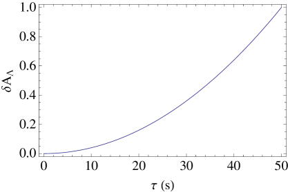
Figure 3: Contribution to the amplitude of the wave form due to $\Lambda$, $\delta A_{\Lambda}$, for a typical neutron star–neutron star inspiral in the LIGO band. We have considered $\Lambda=10^{-52}\mathrm{m}^{-2}$, a frequency of $f(=\omega/2\pi)=200~{}\mathrm{Hz}$ and a duration of $10^{4}$ cycles. The amplitude is normalized as to be unitary at the end of the detection, when $\delta A_{\Lambda}\simeq 3\times 10^{-34}$; time units are in seconds.

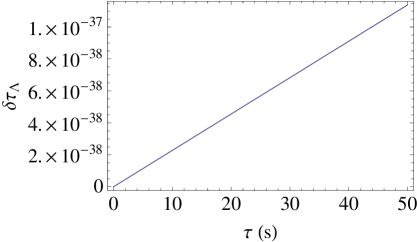
Figure 4: The same as fig. 3 for the phase shift $\delta\tau_{\Lambda}$. The time unit on the $y$-axis is given by the unperturbed period, $T=2\pi/\omega 5\times 10^{-3}~{}\mathrm{s}$.

Let $\tau_{\mathrm{day}}$ denote the length of the measurement in days. Then the relative weight of the leading $\Lambda$–dependent term for this example is of order

$$\left|\frac{\Lambda c^{2}\tau^{2}}{48\pi}\right|\approx 5\cdot 10^{-28}\cdot\tau_{\mathrm{day}}^{2}.$$ (46)

If the amplitude of the wave does not vanish before the measurement starts, i. e. if the function $f(t)$ unlike $\varphi(t)$ does not vanish for $t<0$, we gather from the general result (IV) that then the leading term proportional to $\tau^{3}$ is present. The relative weight of this term depends on $\omega$ and thus on the type of the source of radiation. We have

$$\left|\frac{\Lambda}{24\pi}\cdot\frac{\omega c^{2}\tau^{3}}{3}\right|\approx 2.5\cdot 10^{-23}\cdot\omega_{\mathrm{Hz}}\tau_{\mathrm{day}}^{3},$$ (47)

where $\omega_{\mathrm{Hz}}$ measures the frequency in Hertz. For compact sources $\omega$ is related to the size and the mass of the source. The size is bounded below by the Schwarzschild radius of the mass. This yields an upper bound on the frequency given by $\omega\approx 10^{4}\mathrm{Hz}$ Flanagan and Hughes (2005). Equation (47) then leads in the best case to

$$\left|\frac{\Lambda}{24\pi}\cdot\frac{\omega c^{2}\tau^{3}}{3}\right|\lesssim 2.5\cdot 10^{-19}\cdot\tau_{\mathrm{day}}^{3}.$$ (48)

In principle the effects of $\Lambda$ are measurable if the signal to noise ratio (SNR) of the detector is sufficiently large. Present as well as planned observatories however do not feature the required accuracy. For example the Earthbounded detector advanced LIGO achieves a $\textrm{SNR}\approx 10$ for the inspiral of compact objects of mass $m\approx 10^{2}M_{\odot}$ at a frequency $\omega\approx 10^{2}\mathrm{Hz}$ McWilliams and Baker (2006). Then the detectability of the effects of $\Lambda$ may be measured by

$$\textrm{SNR}_{\Lambda,\textrm{LIGO}} \approx 2.5\cdot 10^{-23}\cdot\omega_{\mathrm{Hz}}\tau_{\mathrm{day}}^{3}\textrm{SNR}_{0,\textrm{LIGO}}$$

$$\approx 2.5\cdot 10^{-20}\tau_{\mathrm{day}}^{3}.$$

The planned spacebased observatory LISA on the other hand is expected to reach a $\textrm{SNR}\approx 10^{4}$ for the inspiral of supermassive black holes with $m\approx 10^{6}M_{\odot}$ at a frequency $\omega\approx 10^{-2}\mathrm{Hz}$ McWilliams and Baker (2006). This yields

$$\textrm{SNR}_{\Lambda,\textrm{LISA}} \approx 2.5\cdot 10^{-23}\cdot\omega_{\mathrm{Hz}}\tau_{\mathrm{day}}^{3}\textrm{SNR}_{0,\textrm{LISA}}$$

$$\approx 2.5\cdot 10^{-21}\tau_{\mathrm{day}}^{3}.$$

The corresponding SNR for the example with $f=\varphi$ can be calculated by considering (46) instead of (47). Then

$$\textrm{SNR}_{\Lambda,\textrm{LIGO}} \approx 5\cdot 10^{-28}\cdot\tau_{\mathrm{day}}^{2}\textrm{SNR}_{0,\textrm{LIGO}}$$

$$\approx 5\cdot 10^{-27}\tau_{\mathrm{day}}^{2}.$$

respective

$$\textrm{SNR}_{\Lambda,\textrm{LISA}} \approx 5\cdot 10^{-28}\cdot\tau_{\mathrm{day}}^{2}\textrm{SNR}_{0,\textrm{LISA}}$$

$$\approx 5\cdot 10^{-24}\tau_{\mathrm{day}}^{2}.$$

For $\tau_{\mathrm{day}}=1$ e. g., the aforesaid observatories would have to increase their accuracy by at least twenty orders of magnitude in order to detect the effects of $\Lambda$ on the waveform radiated by the inspirals mentioned above. Thus even for a long but realistic period of measurement it is not possible to detect the effects of $\Lambda$ within the existing technology.

VI Conclusions

We investigated the linearised Einstein’s equations with a cosmological term and derived explicit expressions for the corrections to the plane gravitational waves up to linear order in $\Lambda$. The polarization states of a wave remain unchanged in the presence of the cosmological term. This conclusion is consistent with the result obtained in Bičák and Podolský (1999a, b). The amplitude as well as the frequency (for periodic radiation) though are modified with increasing time. However, these effects are very tiny and thus not detectable by present or planned detectors.

We point out that one can not rule out the possibility that nonlinear effects originating from terms proportional to $h_{\mu\nu,\lambda}h_{\rho\sigma,\tau}$ in an expansion (II) could lead to effects on the waveform similar in size as the ones due to the cosmological term. However, as discussed for instance in Flanagan and Hughes (2005), such a perturbation term can be split into a slowly varying piece, and a rapidly varying one. The latter one would induce modifications on a much shorter timescale than the contribution due to the cosmological constant as considered here, and should thus be easily discriminated. On the other hand the long timescale contribution would modify the background. However, its timedepence might be different from the one due to the cosmological constant and thus making it still possible to distinguish the various effects. A detailed analysis of effects due to quadratic terms in $h$ is certainly quite involved and beyond the scope of the present work.

A mentionable phenomenon is eventually the connection between the cosmological constant and the mass of the graviton. Mass terms characterize Klein–Gordon equations and are connected to the dispersion relation. We do not go further into this question and refer to Freund et al. (1969); Novello and Neves (2003); Liu (2004).

Acknowledgments

M.S. is supported by the Swiss national science Foundation and by the Tomalla Foundation. We thank the referee for some clarifying suggestions.

References

• Peebles and Ratra (2003) P. J. Peebles and B. Ratra, Reviews of Modern Physics 75, 559 (2003), eprint arXiv:astro-ph/0207347.
• Jetzer and Sereno (2006) P. Jetzer and M. Sereno, Phys. Rev. D 73, 044015 (2006), eprint arXiv:astro-ph/0601612.
• Sereno and Jetzer (2006) M. Sereno and P. Jetzer, Phys. Rev. D 73, 063004 (2006), eprint arXiv:astro-ph/0602438.
• Sereno and Jetzer (2007) M. Sereno and P. Jetzer, Phys. Rev. D 75, 064031 (2007), eprint arXiv:astro-ph/0703121.
• Islam (1983) J. N. Islam, Physics Letters A 97, 239 (1983).
• Kerr et al. (2003) A. W. Kerr, J. C. Hauck, and B. Mashhoon, Classical and Quantum Gravity 20, 2727 (2003), eprint arXiv:gr-qc/0301057.
• Wright (1998) E. L. Wright, ArXiv Astrophysics e-prints (1998), eprint astro-ph/9805292.
• Iorio (2006) L. Iorio, International Journal of Modern Physics D 15, 473 (2006), eprint arXiv:gr-qc/0511137.
• Rindler and Ishak (2007) W. Rindler and M. Ishak, Phys. Rev. D 76, 043006 (2007), eprint arXiv:0709.2948.
• Sereno (2008) M. Sereno, Phys. Rev. D 77, 043004 (2008), eprint arXiv:0711.1802.
• Balaguera-Antolínez and Nowakowski (2005) A. Balaguera-Antolínez and M. Nowakowski, Astron. Astrophys. 441, 23 (2005), eprint arXiv:astro-ph/0511738.
• Ozsváth et al. (1985) I. Ozsváth, I. Robinson, and K. Rózga, Journal of Mathematical Physics 26, 1755 (1985).
• Bičák and Podolský (1999a) J. Bičák and J. Podolský, Journal of Mathematical Physics 40, 4495 (1999a), eprint arXiv:gr-qc/9907048.
• Bičák and Podolský (1999b) J. Bičák and J. Podolský, Journal of Mathematical Physics 40, 4506 (1999b), eprint arXiv:gr-qc/9907049.
• Lu (1988) H.-Q. Lu, Acta Astrophysica Sinica 8, 94 (1988).
• Polarski (1989) D. Polarski, Classical and Quantum Gravity 6, 893 (1989).
• Dafermos and Rodnianski (2007) M. Dafermos and I. Rodnianski, ArXiv e-prints 709 (2007), eprint 0709.2766.
• Yagdjian and Galstian (2007) K. Yagdjian and A. Galstian, ArXiv e-prints 710 (2007), eprint 0710.3878.
• Bony and Hafner (2007) J.-F. Bony and D. Hafner, ArXiv e-prints 706 (2007), eprint 0706.0350.
• Straumann (2004) N. Straumann, General relativity with applications to astrophysics (Springer Texts and monographs in physics. Berlin: Springer, 2004).
• Landau and Lifshitz (1992) L. D. Landau and E. M. Lifshitz, Klassische Feldtheorie (Lehrbuch der theoretischen Physik. Berlin: Akademie-Verlag, 12. Auflage, 1992).
• Flanagan and Hughes (2005) É. É. Flanagan and S. A. Hughes, New Journal of Physics 7, 204 (2005), eprint arXiv:gr-qc/0501041.
• de Sitter (1917) W. de Sitter, Monthly Notices of the Royal Astronomical Society 78, 3 (1917).
• McWilliams and Baker (2006) S. T. McWilliams and J. G. Baker, in Laser Interferometer Space Antenna: 6th International LISA Symposium, edited by S. M. Merkovitz and J. C. Livas (2006), vol. 873 of American Institute of Physics Conference Series, pp. 110–114.
• Freund et al. (1969) P. G. O. Freund, A. Maheshwari, and E. Schonberg, Astrophys. J.  157, 857 (1969).
• Novello and Neves (2003) M. Novello and R. P. Neves, Classical and Quantum Gravity 20, L67 (2003), eprint arXiv:gr-qc/0210058.
• Liu (2004) L. Liu, ArXiv e-prints (2004), eprint gr-qc/0411122.