Possible superconducting symmetry on doped $J_{1}$-$J_{2}$ model

Abstract

By making use of renormalized mean-field theory, we investigate possible superconducting symmetries in the ground states of ${t_{1}}$-${t_{2}}$-${J_{1}}$-${J_{2}}$ model on square lattice. The superconducting symmetries of the ground states are determined by the frustration amplitude $t_{2}/t_{1}$ and doping concentration. The phase diagram of this system in frustration-doping plane is given. The order of the phase transitions among these different superconducting symmetry states of the system is discussed.

Frustrated magnets based on transition metals have attracted much theoretical and experimental effort in the past years, a variety of exotic quantum effectsY.Taguchi ; co ; kos ; huang expected when competitive interactions lead a system into a frustrated state, where it is impossible to satisfy all the pair interactions simultaneously. One of the most simple yet very important systems is spin-1/2 Heisenberg model on a square lattice with competing nearest $J_{1}$ and next-nearest $J_{2}$ neighbor spin interactions. Despite its simplicity, it is not only in its own right academically interesting, but also practically provides a window for looking inside into the superconductivity mechanism. Recently found vanadium-based compounds have provided experimental realizations of $J_{1}$-$J_{2}$ model with $J_{2}/J_{1}\sim 1$ melzi ; carretta ; rosner ; bombardi and again have stimulated research on this charming system.

As is known, a single layer in undoped cuprate high-$T_{c}$ compounds are well described by a square-lattice Heisenberg model displaying long-range antiferromagnetic Néel order. The common belief is that upon doping, this long range order is destroyed and a different non-magnetic phase sets in, which, accompanied by fluctuations, turns the system into superconducting phase. One idea suggests that the effect of doping in destroying the Néel order might be accounted for by the introduction of frustration in original Heisenberg model inui . Following this suggestion, many works had been focused on finding such phases in frustrated quantum magnets chandra ; dagotto ; read-sachdev ; chandra-coleman-larkin . Recently, the half-filled Hubbard model with both nearest neighbor and next-nearest-neighbor hopping term has been investigated nevidomskyy . This model in the large $U$ limit is equivalent to $J_{1}$-$J_{2}$ model. In that paper, variational cluster approach shows that $d_{x^{2}-y^{2}}$-wave superconductivity can also occur at half-filling when the Hubbard system is under pressure provided that the frustration and the on-site repulsion are not too large.

However, there is another issue which is worth while to be investigated: possible superconducting symmetries of $J_{1}$-$J_{2}$ model under doping.

At half-filling $J_{1}$-$J_{2}$ model respectively exhibits two long-range magnetic orders in two distinct limit: a) the Néel phase in the limit of $J_{2}/J_{1}\rightarrow 0$; b) the so called collinear phase misguich with ordering wave vector $(\pi,0)$ or $(0,\pi)$ in the limit of $J_{2}/J_{1}>>1$. Frustration makes the system highly degenerated in the intermediate range and may dramatically suppresses the magnetic long range order xu-ting ; oguchi ; igarashi ; gochev ; dotsenko . Hence together with doping, frustration may provide the system exotic superconducting symmetries over a broad range of doping and frustration.

In this work we investigate superconducting symmetry of the ground state of doped ${J_{1}}$-${J_{2}}$ model, i.e. $t_{1}$-$t_{2}$-$J_{1}$-$J_{2}$ model. To investigate the properties of the ground state, a simple yet powerful method is the renormalized mean-field theory (RMFT) anderson-lee ; zhang88 in which the kinetic and superexchange energies are renormalized by different doping-dependent factors $g_{t}$ and $g_{s}$, respectively. Despite of the simplicity of this method, it can lead to semi-quantitative even quantitative explanation of some ground state properties of cuprate superconductors anderson-lee ; zhang-rice ; zhang88 . In this letter, with the help of RMFT, we show that the superconducting symmetry of the ground state varies among different types when tuning the frustration amplitude and doping concentration of the system.

Model — The Hamiltonian of the $t_{1}$-$t_{2}$-$J_{1}$-$J_{2}$ model takes the form of

$$H = \hat{P_{d}}H_{t}\hat{P_{d}}+H_{s}\;\;,$$

$$H_{t} = -t_{1}\sum_{\langle nn\rangle\sigma}c^{{\dagger}}_{i\sigma}c_{j\sigma}-t_{2}\sum_{\langle nnn\rangle\sigma}c^{{\dagger}}_{i\sigma}c_{j\sigma}+h.c.\;\;,$$

$$H_{s} = J_{1}\sum_{\langle nn\rangle}\mathbf{S}_{i}\cdot\mathbf{S}_{j}+J_{2}\sum_{\langle nnn\rangle}\mathbf{S}_{i}\cdot\mathbf{S}_{j}\;\;,$$ (1)

$\hat{P_{d}}=\prod\limits_{i}(1-n_{i\uparrow}n_{i\downarrow})$ is the Gutzwiller projection operator zhang88 which removes totally the doubly occupied states. $t_{1}$ and $t_{2}$ are nearest-neighbor and next-nearest-neighbor hopping amplitude. When they are all positive, the Hamiltonian represents hole doping case. The electron doping case can be achieved via particle-hole transformation, changing the sign of $t_{2}$ while keeping the sign of $t_{1}$ unchanged liu-trivedi . $J_{1}$ and $J_{2}$ are respectively the nearest-neighbor and next-nearest-neighbor antiferromagnetic coupling constants, they raise frustration in the system. We use $t_{1}$ as the energy unit and set $\mathrm{t}_{1}/\mathrm{J}_{1}=3$ for conventional reason kim-shen ; coldea , ${J_{2}}/{J_{1}}=({t}_{2}/{t}_{1})^{2}$ since the superexchanges have relations of ${J}=4{t}^{2}/U$ with hopping parameters in the large Hubbard ${U}$ limit. And we take $\eta={t_{2}}/{t_{1}}$ as frustration amplitude.

Method — Renormalized mean-field theory. In the frame of RMFT, to investigate the ground state of the above mentioned Hamiltonian, the trial state is suggested to be a projected $BCS$ state $|\Psi\rangle=P_{d}|\Psi_{0}\rangle$, where $|\Psi_{0}\rangle=\prod_{k}(u_{k}+\upsilon_{k}c^{\dagger}_{k\uparrow}c^{\dagger}_{-k\downarrow})|0\rangle$. And the projection operator is taken into account by a set of renormalized factors gutzwiller ; vollhardt ; ogawa , i.e. we have $\langle\psi|H|\psi\rangle=\langle\psi_{0}|H^{\prime}|\psi_{0}\rangle=\langle\psi_{0}|g_{t}H_{t}+g_{s}H_{s}|\psi_{0}\rangle$. In homogenous case the renormalized factors zhang88 $g_{t}=2\delta/(1+\delta)$ and $g_{s}=4/(1+\delta)^{2}$.

Minimize the quantity $W=\langle H^{\prime}-\mu\sum_{i\sigma}c_{i\sigma}^{\dagger}c_{i\sigma}\rangle_{0}$ with respect to $u_{k}$ and $\upsilon_{k}$, and introduce two mean-field parameters $\Delta_{\tau}=\langle c^{{\dagger}}_{i\uparrow}c^{{\dagger}}_{i+\tau\downarrow}-c^{{\dagger}}_{i\downarrow}c^{{\dagger}}_{i+\tau\uparrow}\rangle_{0}$ and $\xi_{\tau}=\sum_{\sigma}\langle c^{{\dagger}}_{i\sigma}c_{i+\tau,\sigma}\rangle_{0}$, where $\tau$ indicates four different bond directions sketched in Fig.1, we get the coupled gap equations as follows

$$\Delta_{\tau} = N_{s}^{-1}\sum_{k}\cos{k_{\tau}}\Delta_{\vec{k}}/E_{\vec{k}}\;\;,$$ (2)

$$\xi_{\tau} =- N_{s}^{-1}\sum_{k}\cos{k_{\tau}}\xi_{\vec{k}}/E_{\vec{k}}\;\;,$$ (3)

where $\Delta_{\vec{k}}=\sum_{\tau}\Delta_{\tau}{J}_{\tau}/{J}_{1}\cos{k_{\tau}}$, $\xi_{\vec{k}}=\bar{\varepsilon}_{\vec{k}}-\sum_{\tau}\xi_{\tau}{J}_{\tau}/{J}_{1}\cos{k_{\tau}}$, $E_{\vec{k}}=\sqrt{\xi_{\vec{k}}^{2}+|\Delta_{\vec{k}}|^{2}}$, $N_{s}$ is the total number of sites. In the above equations $\bar{\varepsilon}_{\vec{k}}=(-2g_{t}{t}_{1}\sum_{\tau}{t}_{\tau}/{t}_{1}\cos{k_{\tau}}-\tilde{\mu})/(\frac{3}{4}g_{s}{J})$ and $\tilde{\mu}=\mu+N_{s}^{-1}\langle\frac{\partial H^{\prime}}{\partial\delta}\rangle_{0}.$ These gap equations should be solved simultaneously with $\delta=N_{s}^{-1}\sum_{\vec{k}}\xi_{\vec{k}}/E_{\vec{k}}$, the resulting $\Delta$’s determine the symmetry of possible superconductivity.

Although the RMFT cannot provide us a true picture of the system in exact half-filling case, the symmetries of gap parameters obtained at that point will not change under small doping anderson-lee . Thus, in order to investigate possible superconducting symmetries of the system under doping, our strategy is following: at first, we solve the gap equation at half filling, find out the possible symmetries of the mean-field parameters. These symmetry states may degenerate at half-filling. Then we switch on the doping, compare the energies of different symmetry states, we can find the true ground states for different doping level and frustration amplitude.

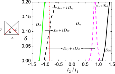
Figure 1: Left picture is schematic structure of ${t_{1}}$-${t_{2}}$-${J_{1}}$-${J_{2}}$ model lattice. We use $a,b$ to distinguish the two different orientation diagonal bond. Right picture is phase diagram of this lattice, dashed lines are boundary of first order phase transition.

At half filling, energy if per site is $-\frac{3}{8}g_{s}J\sum_{k}E_{k}$, with the ansatz that $E_{k}$ of ground state energy can be written as a summation of square terms of cosine functions, after some calculation, we find that several symmetry states come out, including: (1) $D_{xy}+is_{ab}$-wave state degenerates with $D_{xy}+iD_{ab}$-wave state, both of them have $\xi_{a,b}=0$; (2) $D_{ab}+iD_{xy}$-wave state degenerates with $D_{ab}+is_{xy}$-wave state, $\xi_{x,y}=0$ in both states. Here $i$ means that the difference between the phase $\phi_{a}$ of $\Delta_{a}$ and the phase $\phi_{x}$ of $\Delta_{x}$ is $|\phi_{a}-\phi_{x}|=\pi/2$, we use $D_{\tau_{1}\tau_{2}}$ and $s_{\tau_{1}\tau_{2}}$ to denote $d$-wave symmetry and $s$-wave symmetry on direction $\tau_{1}$ and $\tau_{2}$ respectively.

When changing the doping level and the frustration amplitude, these superconducting symmetries compete, and energetically, each occupies a specific region in the phase diagram, as shown in Fig.1. In this phase diagram dashed line are boundary of the first order phase transition where mean-field parameters change suddenly. The bold lines show second order phase transitions. Left picture in Fig.1 is a cartoon sketch of the lattice structure that we discuss, $a$ and $b$ denote the two different diagonal bond. In the following, we are going to discuss the phase diagram for positive and the negative $t_{2}/t_{1}$ case in more detail.

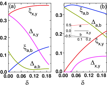
Figure 2: Figure(a) shows mean-field parameters of $D_{xy}+iD_{ab}$ state as function of $\delta$ for $\eta=\sqrt{0.6}$. Figure(b) shows parameter functions for $\eta=\sqrt{1.5}$, the inset picture shows phase of pairing parameters, its unit is $\pi$.

Positive $\eta$ cases. — For $\eta<\sqrt{0.5}$, as expected, although the next nearest neighbor interaction frustrates the system, it does not destroy the $D$-wave superconducting symmetry state with $\Delta_{x}=-\Delta_{y}$ and $\Delta_{a,b}=0$ for all doping level under investigation. For $\eta>\sqrt{0.5}$, pairing on diagonal links should be considered seriously.

RMFT calculation shows that when the frustration amplitude falls in the range of $\sqrt{0.5}\leq\eta<\sqrt{0.7}$, $D_{xy}+iD_{ab}$-wave state with $|\Delta_{x,y}|>|\Delta_{a,b}|$ is the most energetically favored state in the small doping region. In order to show the dependence on the doping concentration, as an example, we take $\eta=\sqrt{0.6}$ and plot $D_{xy}+iD_{ab}$-wave parameters in Fig.2(a). With increasing $\delta$, $\Delta_{a,b}$ decreases rapidly. One can see from phase diagram Fig.1 that after $\delta=0.06$, $D_{xy}$-wave state is energetically more favored, and there is a sudden change of $\Delta_{a,b}$ in this transition.

For about $\sqrt{0.8}<\eta<\sqrt{1.1}$ in small doping level stable state is still $D_{xy}+iD_{ab}$-wave state, however, in relatively high doping level another mixed superconducting symmetry state of $s_{xy}+iD_{ab}$-wave dominates. Again, in order to illustrate the dependence on doping level, we take $\eta=\sqrt{0.9}$ and plot the parameters for $D_{xy}+iD_{ab}$ symmetry and $s_{xy}+iD_{ab}$ symmetry in Fig.3(a) and Fig.3(b), respectively. Inset of Fig.3(b) shows the phases of $\Delta_{\tau}$ in different bond directions, and clearly reflects the symmetry property of the $s_{xy}+iD_{ab}$-wave state. From this inset, we can also see that the phases of $\Delta_{a,b}$ is slightly away from $\pi/2$. By comparing the energies of these two different states, the calculation shows that a first order phase transition from $D_{xy}+iD_{ab}$-wave state to $s_{xy}+iD_{ab}$-wave state occurs when increasing the doping level $\delta$ across $0.06$. When $\eta$ is tinily larger than $1$, in very small doping region stable state most likely is another type of $D_{ab}+iD_{xy}$-wave with $|\Delta_{a,b}|>|\Delta_{x,y}|$, it occupies really an extremely small area and can not be shown explicitly in our phase diagram.

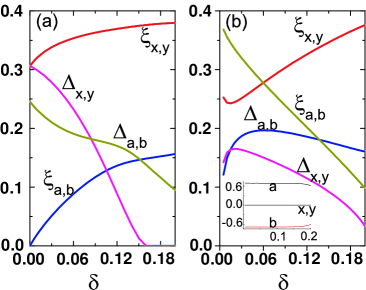
Figure 3: (color online) For $\eta=\sqrt{0.9}$, Fig.(a) shows mean-field parameters of $D_{xy}+iD_{ab}$-wave state, while Fig.(b) shows that of $s_{xy}+iD_{ab}$-wave, the inset of (b) shows the phases of its pairing parameters.

In the region of $\sqrt{1.2}<\eta<\sqrt{2}$, stable state is $D_{ab}$-wave in small doping and will change to $s_{xy}+iD_{ab}$-wave state when increasing the doping level with the corresponding phase transition being second order. In Fig.2(b) we show the case of $\eta=\sqrt{1.5}$, it is clear that the parameters vary smoothly from $D_{ab}$-wave type to $s_{xy}+iD_{ab}$-wave type when increasing $\delta$. Inset of Fig.2(b) clearly shows that in $s_{xy}+iD_{ab}$-wave state phase difference of $\Delta_{a,b}$ is not exactly $\pi$ and varies slowly with doping concentration.

For very large $\eta$, it is reasonable to expect a state with $d$-wave pairing only on diagonal bonds, i.e. the state is $D_{ab}$-wave.

Negative $\eta$ case. — As in the positive $\eta$ case, when $|\eta|$ takes small value, roughly smaller than $\sqrt{0.5}$, superconducting symmetry of the system is conventional $d$-wave on plaquette bonds.

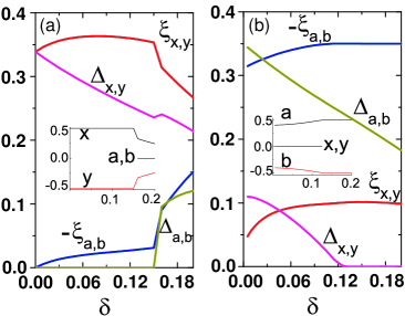
Figure 4: (color online) Figure(a) shows mean-field parameters amplitude of stable state as function of $\delta$ for $\eta=-\sqrt{0.6}$, figure(b) shows parameter function of stable state for $\eta=-\sqrt{1.2}$, the inset of (a,b) shows the phase of $\Delta$.

For $-\sqrt{0.7}<\eta<-\sqrt{0.5}$, the $D_{xy}$-wave symmetry changes into $s_{ab}+iD_{xy}$-wave state when increasing doping level with the phase transition being first order. It should be emphasized that the phase difference between $\Delta_{x}$ and $\Delta_{a}$ in the latter state is less than $\pi/2$ and decreases with increasing doping level. Fig.4(a) shows that for $\eta=-\sqrt{0.6}$, when $\delta>0.16$, $D_{xy}$-wave state discontinuously changes to $s_{ab}+iD_{xy}$-wave state. Inset shows the phase of pairing parameters, at the critical point symmetry of superconductivity changes suddenly.

When $-\sqrt{1.5}<\eta<-\sqrt{1.1}$, $D_{ab}$-wave is the stable state in high doping level while in small doping level stable state is $s_{xy}+iD_{ab}$-wave symmetry. $\eta=-\sqrt{1.2}$ case is shown explicitly in Fig.4(b) as an example. With increasing $\delta$ pairing on diagonal bonds $\Delta_{x,y}$ decrease to zero rapidly and $s_{xy}+iD_{ab}$-wave state varies to $D_{ab}$-wave smoothly through a second order phase transition. $D_{ab}$-wave state occupies more range of $\delta$ when increasing $|\eta|$ till $|\eta|=\sqrt{1.5}$, after that $D_{ab}$ is the only stable one for all doping level.

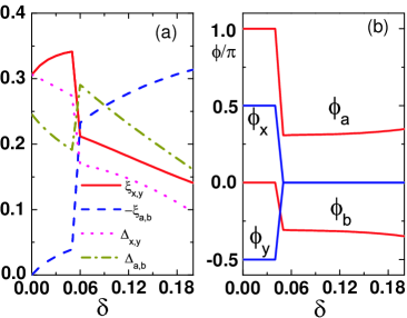
Figure 5: (color online) Figure(a) shows mean-field parameters amplitude of stable state as function of $\delta$ for $\eta=-\sqrt{0.9}$, figure(b) shows phase of pairing parameters. At the critical point symmetry of superconductivity change for $D_{xy}+iD_{ab}$ to $s_{xy}+iD_{ab}$ wave state.

For $-\sqrt{1.1}<\eta<-\sqrt{0.7}$, in small doping level $D_{xy}+iD_{ab}$ state has more energy gain while $s_{xy}+iD_{ab}$ is more stable at higher doping level. Fig.5(a) shows how parameter amplitudes varied with doping concentration at $\eta=-\sqrt{0.9}$ for best energy stable state and Fig.5(b) shows the phase changing of stable state. The sudden changes of the parameter amplitudes and phases clearly indicate that the phase transition here is first order.

Summary and discussion —In summary, we have investigated the possible superconducting symmetries of frustrated ${t_{1}}$-${t_{2}}$-${J_{1}}$-${J_{2}}$ model by RMFT method. In terms of frustration amplitude $t_{2}/t_{1}$ and doping concentration $\delta$ a phase diagram for possible superconducting symmetry states has been presented. We have shown that in weakly and strongly frustrated cases pure $d$-wave states are on plaquette or diagonal bonds, respectively. When $t_{1}$ and $t_{2}$ are comparable, pairing parameters on plaquette bonds and diagonal bonds are both finite and mixed symmetry states such as $D+iD$, $D+is$ appear. Each symmetry state occupies a specific region in the phase diagram, transitions between these states are the first order or second order, the latter one corresponding to relatively large $J_{2}$. The two kinds of time-reversal broken mixed states are consistent with those found in two-dimensional Fermi liquid with attractive interaction in both $s$ and $D$ channel fermi , $D+is$ time-reversal broken state may also appear in the pseudogap phase timere . We hope that our calculation may shed some new light on the study of mechanism of superconducting order in high-$T_{c}$.

Acknowledgment — Work supported by NSF of china Nos.10747145, and 10575068.

References

- (1) Y. Taguchi, Y. Oohara, H. Yoshizawa, N. Nagaosa, and Y. Tokura, Science 291, 2573 (2001).
- (2) K. Takada, H. Sakurai, E. Takayama-Muromachi, F. Lzumi, R. A. Dilanina, and T. Sasaki, Narure(London) 422, 53 (2003).
- (3) S. Yonezawa, Y. Muraoka, Y. Matsushita, and Z. Hiroi, J. Phus :condens. Matter, 75, L9 (2004).
- (4) H. X. Huang, Y. Q. Li, J. Y. Gan, Y. Chen and F. C. Zhang, Phys. Rev. B 75, 184523 (2007).
- (5) R. Melzi, P. Carretta, A. Lascialfari, M. Mambrini, M. Troyer, P. Millet and F. Mila, Phys. Rev. Lett. 85, 1318 (2000).
- (6) P. Carretta, N. Papinutto, C. B. Azzoni, M. C. Mozzati, E. Pavarini, S. Gonthier, and P. Millet, Phys. Rev. B 66, 094420 (2002); P. Carretta, R. Melzi, N. Papinutto and P. Millet, Phys. Rev. Lett. 88, 047601 (2002).
- (7) H. Rosner, R. R. P. Singh, W. H. Zheng, J. Oitmaa, S.-L. Drechsler, and W. E. Pickett, Phys. Rev. Lett. 88, 186405 (2002); H. Rosner, R. R. P. Singh, W. H. Zheng, J. Oitmaa, and W. E. Pickett, Phys. Rev. B 67, 014416 (2003).
- (8) A. Bombardi, J. Rodriguez-Carvajal, S. Di Matteo, F. de Bergevin, L. Paolasini, P. Carretta, P. Millet, and R. Caciuffo, Phys. Rev. Lett. 93, 027202(2004).
- (9) M. Inui, S. Doniach, and M. Gabay, Phys. Rev. B 38, 6631 (1988).
- (10) P. Chandra and B. Doucot, Phys. Rev. B 38, 9335 (1988).
- (11) E. Dagotto and A. Moreo, Phys. Rev. Lett. 63, 2148 (1989).
- (12) N. Read and S. Sachdev, Phys. Rev. Lett. 62, 1694 (1989).
- (13) P. Chandra, P. Coleman, and A.I. Larkin, Phys. Rev. Lett. 64, 88 (1990).
- (14) A. H. Nevidomskyy, C. Scheiber, D. Sénéchal, and A.-M. S. Tremblay Phys. Rev. B 77, 064427 (2008).
- (15) G. Misguich and C. Lhuillier, arXiv: cond-mat/0310405 (2003).
- (16) J. H. Xu and C. S. Ting, Phys. Rev. B 42, 6861 (1990).
- (17) T. Oguchi and H. Kitatani, J. Phys. Soc. Jpn. 59, 3322 (1990).
- (18) J. Igarashi, J. Phys. Soc. Jpn. 62, 4449 (1993).
- (19) I. G. Gochev, Phys. Rev. B 49, 9594 (1994).
- (20) A. V. Dotsenko and O. P. Sushkov, Phys. Rev. B 50, 13821 (1994).
- (21) P. W. Anderson, P. A Lee, M. Randeria, T. M. Rice, N. Trivedi and F. C. Zhang, J. Phys. Cond. Matt. 16, R755 (2004).
- (22) F. C. Zhang, C. Gros, T. M. Rice and H. Shiba, Supercond. Sci. Tech. 1, 36 (1988).
- (23) F. C. Zhang and T. M. Rice, Phys. Rev. B 37, 3759 (1988).
- (24) J. Liu, N. Trivedi, Y. Lee, B. N. Harmon, and J. Schmalian, Phys. Rev. Lett. 99, 227003 (2007).
- (25) C. Kim, P. J. White, Z.-X. Shen, T. Tohyama, Y. Shibata, S. Maekawa, B. O. Wells, Y. J. Kim, R. J. Birgeneau, and M. A. Kastner, Phys. Rev. Lett. 80, 4245 (1998).
- (26) R. Coldea, S. M. Hayden, G. Aeppli, T. G. Perring, C. D. Frost, T. E. Mason, S. -W. Cheong, and Z. Fisk, Phys. Rev. Lett. 86, 5377 (2001).
- (27) M. C. Gutzwiller, Phys. Rev. 137, A1726(1965).
- (28) D. Vollhardt, Rev. Mod. Phys. 56, 99 (1984).
- (29) T. Ogawa, K. Kanda and T. Matsubara, Prog. Theor. Phys. 53, 614 (1975).
- (30) H. Aoki, J. Phys: Condensed Matter 16, V1 (2004).
- (31) K. A. Musaelian, J. Betouras, A. V. Chubukov and R. Joynt, Phys. Rev. B. 53, 3598 (1996).
- (32) R. P. Kaur and D. F. Agterberg, Phys. Rev. B 68, 100506(R) (2003).