Complex extension of potentials and trajectories of poles of the $S$-matrix element
in the complex momentum plane

Abstract

Searching for infrastructure of the quantum mechanical system, we study trajectories of the $s$-wave poles of the $S$-matrix element with respect to a real phase $\alpha$ in the complex momentum plane for a complex extension of real potentials by a phase factor ${e}^{{i}\alpha}$. This complex extension relates the pole spectrum of the physical system with a potential to the spectrum of another system with the potential of the same shape but of opposite sign. There appear trajectories with the periodicity of $2\pi,4\pi$, and $\infty$. The appearance of non-recurrent behavior of the trajectory for the change of phase $\Delta\alpha=2\pi$ is closely related with the existence of resonance poles for real repulsive potentials. Dynamical changes of trajectory structure are examined.

I Introduction

The hermitian requirement for the Hamiltonian of quantum mechanical system assures the reality of the energy eigenvalues with normalizable wave functions, giving the unitary system. Extensions of hermitian real potentials to non-hermitian complex potentials have been made mainly for three purposes.

The first utilizes complex potentials for representing phenomenologically effects of inelastic processes on elastic scattering known as the optical-potential model bltt ; hdgsn . The second is to generalize the standard quantum mechanics from the standpoint that the requirement of the reality for the potential is too restrictive complexqm . These two are directly associated with non-hermitian potentials.

The third covers attempts which use complex extensions as tools of calculation for systems with real potentials, developed and widely used to evaluate the energy and width of resonances appearing in various fields of physics msyv ; riss ; kkln .

The infrastructure of the physical system with complex potential has been investigated in its various aspects. There seems, however, still to exist some structure studied not fully. It will be worthwhile to clarify some properties of the solutions of Scrödinger equation with complex potentials for further development of these studies involving complex potentials. Here we present an analysis in this direction.

We consider a system with a real potential by extending it with a phase rotation factor $e^{i\alpha}$ where $\alpha$ is a real parameter. We search for some global structure of the quantum system with thus complex-extended potential. By the phase rotation of the potential two physical systems of real potentials of opposite signatures are connected. In other words, there is one complex system which interfaces the real world at $\alpha=n\pi$ for $n=0,\pm 1,\pm 2,\ldots$. This is something like to regard the electron state and the positron state in the Coulomb potential as one hyper-system, though we are not intending the extension in such a direction.

The pole spectrum of a system characterizes the system. In this paper we examine specifically the behavior of poles of scattering amplitude of a particle in potentials. By changing the value of phase $\alpha$ from zero, bound-state and antibound-state poles leave the imaginary axis of the complex momentum plane and resonance poles change their locations in the complex momentum plane.

Since a pole is neither annihilated nor created unless it meets other singularities in the complex momentum plane, we can unambiguously trace each of poles giving its trajectory. This establishes the correspondence between the poles generated by the two real potentials which are the same except their signatures, exposing the pole structure for complex potentials.

In Sec. II we briefly summarize some basic properties of the $S$-matrix for complex potentials. In Sec. III we study stability of trajectories for the potential strength and examine how mutual transformations occur between different trajectories. Some remarks are given in Sec. IV.

II Some properties of the $S$-matrix

We consider a particle of mass $m$ in a complex central scalar potential $V(r)$ with finite range. The time-independent Schrödinger equation for the wave function $\phi({\bf r})$ of the particle is in units of $\hbar=c=1$

$$\left[-\frac{\nabla^{2}}{2m}+V(r)\right]\phi({\bf r})=E\phi({\bf r})\,,$$ (1)

where $E$ is the energy of the particle.

Here the complex potential is assumed to be given by

$$V(r)={e}^{{i}\alpha}V_{0}(r)\,,$$ (2)

where $V_{0}(r)$ is a real function of $r$ and $\alpha$ is a real phase parameter. For $\alpha=2n\pi\,(n=0,\pm 1,\pm 2,...)$ the system represents the same physical world. Similarly, for $\alpha=(2n+1)\pi$ we have the system characterized by the potential of the same shape and of opposite sign.

We expand the wave function $\phi({\bf r})$ into the partial waves and denote the radial part of the wave function for the state with angular momentum $l$ by $u_{l}(r)/r$. The equation for $u_{l}(r)$ is

$$\biggl{\{}\frac{\mathrm{d}^{2}}{\mathrm{d}r^{2}}+2m\bigl{[}E-V(r)\bigr{]}-\frac{l(l+1)}{r^{2}}\biggr{\}}u_{l}(r)=0\,.$$ (3)

Let $u_{l}^{(+)}(r)$ and $u_{l}^{(-)}(r)$ are the outgoing and the incoming wave solution, respectively. The wave function $u_{l}(r)$ in the outer interaction-free region is given in terms of $u_{l}^{(+)}(r)$ and $u_{l}^{(-)}(r)$ by

$$u_{l}(r)=S_{l}u_{l}^{(+)}(r)-u_{l}^{(-)}(r)\,,$$ (4)

where $S_{l}$ is the $S$-matrix element for the angular momentum $l$.

Here we summarize some analytic properties of the $S$-matrices for the complex finite-range potentials kkln . The momentum of the particle $k$ outside the range of the potential is given by $k=(2mE)^{1/2}$. We study the pole structure of the $S$-matrix element in the complex momentum $k$ plane.

For the complex finite-range potential the $S$-matrix element with the angular momentum $l$ can be expressed by using the Jost function $f_{l}(k,\alpha)$ by

$$S_{l}(k,\alpha)=\frac{f_{l}(k,\alpha)}{f_{l}(-k,\alpha)}\,.$$ (5)

The Jost function $f_{l}(k,\alpha)$ is an entire function of $k$ for strictly finite-range potential and has no singularities except at infinity. The pole of the $S$-matrix comes from the zero of $f_{l}(-k,\alpha)$. The $S$-matrix element satisfies the following relations

$$S_{l}(k,\alpha)\,\,S_{l}(-k,\alpha)=1\,,$$ (6)

$$S_{l}^{*}(k,-\alpha)=S_{l}(-k^{*},\alpha\bmod 2\pi)\,.$$ (7)

In the complex momentum plane the pole trajectories are symmetric with respect to the imaginary axis. A pole (zero) at the momentum $k$ implies a zero (pole ) at $-k$.

Although we perform the following analysis in the momentum plane, we shortly note on the complex energy plane. In the complex $E$ plane there is a cut starting from the branch point $E=0$ to $\infty$. The Riemann sheet with Im$\,k>0$ is denoted by $I$ and the sheet with Im$\,k<0$ by $II$, which are called the physical and the unphysical sheet, respectively. The zeros and poles have their complex conjugate partners on each of the physical and unphysical sheets and the pole trajectory is symmetric with respect to the real energy axis in the complex energy plane.

There are two classes of poles of the scattering amplitude; fixed poles and moving poles. The fixed-pole spectrum depends only on the shape of the potential and independent of the potential strength as well as the phase parameter $\alpha$, while the location of the moving pole changes in the complex momentum plane with the potential strength and the phase parameter $\alpha$. The fixed pole, though appearing on the positive imaginary axis of the momentum plane (or the negative real axis in the energy plane of physical sheet $I$), is not a physical bound state. We are concerned with the trajectory of the moving pole here.

There appear three kinds of moving poles. The first is the bound-state pole on the positive imaginary axis of the momentum plane (on the negative real axis of the physical sheet $I$), the second is the antibound-state pole on the negative imaginary axis (the negative real energy axis of the unphysical sheet $II$), and the third is the resonance pole in the lower half-plane with positive real part and its conjugate pole with negative real part (or in the lower half-plane of the sheet $II$ and its complex-conjugate partner in the upper half-plane of this sheet) note1 . The conjugate partner is called the antiresonance-state pole.

The moving poles are mutually transformed as the potential strength and the phase $\alpha$ change, with a finite number of the moving poles in the upper half-plane and an infinite number of poles in the lower-half plane. These three kinds of poles should be regarded on the same physical level, though their effects to observable physical processes are greatly different.

A naive expectation might be that any pole will return to its starting point after the change of phase by $\Delta\alpha=2\pi$. As we will see in the following, this occurs only in special situations. This simple problem seems not to have been discussed so far to the knowledge of the present authors.

III Pole trajectories

We examine potentials for which solutions of the Schrödinger equations are available in compact analytical forms. Such potentials are, however, few and the solutions are given mostly only for the $s$-wave at present. Here we study a set of potentials with exponential tail and a finite-range constant potential which is called the square potential here.

The potentials with exponential tail taken in the present analyses can be covered by the expression

$$V_{0}(r)=-U\frac{\exp\left(-r/r_{0}\right)}{\Bigl{[}1+c\exp\left(-r/r_{0}\right)\Bigr{]}}\,.$$ (8)

which may be called here the generalized Hulthén potential htpt . This constitutes a part of the more extended set called the class of Eckart potentials nwtn .

Potentials of this form including the class of Eckart allow us to obtain the analytical solution for the $s$-wave $S$-matrix element in terms of the hypergeometric function. Strictly speaking, the potentials having exponential tail at large distances are not finite-range, but many of properties of the scattering amplitudes of finite-range potentials are shared also by those of the exponential-tail potentials.

We give the trajectory in the complex $k$-plane. Owing to the existence of the branch cut in the $E$-plane, some trajectories look more complicated in the $E$-plane than in the $k$-plane.

As noted in the previous section, all the trajectories might be thought of having the $2\pi$ periodicity. In practice we have $4\pi$ and even aperiodic open trajectories as well as $2\pi$ ones: this is caused by the appearance of the $s$-wave resonance poles for real repulsive potentials. The $s$-wave resonance for the repulsive potential is known, but its physical implication seems rarely to have been discussed in publications.

The transformation of the real potential $V_{0}(r)$ with the phase factor $e^{i\alpha}$ is the self-mapping of the set of all poles onto itself for $\Delta\alpha=\pm 2\pi$ and the set is divided into invariant subsets, each of which corresponds to a closed or open trajectory in the complex $k$-plane.mapping If the potential depth varies, it occurs degeneracy of two virtual states or of a pair of resonance and complex virtual states. This causes rearrangements of trajectories.

In the following analysis $U$ is taken to be positive, giving an attractive potential for $\alpha=0$ note2 .

Here in the numerical calculations we take the mass $m=940$ MeV and the potential-range parameter $r_{0}=1/140$ (MeV)^-1. These values are typical hadronic scales, though we do not intend to make any application to the actual physical processes.

III.1 Potentials with exponential-tail

First we comment on some general features of trajectories given by the potentials with exponential tail. To understand the characteristic features of the change of trajectories with respect to the potential strength $U$, it is necessary to start from very small potential strength. For vanishing $U$ all the moving poles approach the fixed zeros on the negative imaginary momentum axis corresponding to the fixed poles on the positive imaginary axis.

This implies that each pole can be specified by the number $n$ specifying the zero at the momentum

$$k_{n}^{\mathrm{FZ}}=-i\frac{1}{2r_{0}}n\,\,\,\,\,(n=1,2,\dots)\,.$$ (9)

A pole associated with the fixed zero at $k_{n}^{\mathrm{FZ}}$ is designated for the real attractive sector of the potential $(e^{i\alpha}=1)$ as $\mathrm{A}_{n}$, while the corresponding pole for the real repulsive sector $(e^{i\alpha}=-1)$ as $\mathrm{R}_{n}$.

A trajectory of $2\pi$ periodicity is specified by a set of $\mathrm{A}_{n}$ and $\mathrm{R}_{n^{\prime}}$ and we express the trajectory as

$$(\mathrm{R}_{n^{\prime}}-\mathrm{A}_{n})\,\,\,\,(n^{\prime}\geq n)\,.$$ (10)

It will be evident that all the trajectories for very small $U$ are $(\mathrm{R}_{n}-\mathrm{A}_{n})$ with the periodicity 2$\pi$.

A trajectory of $4\pi$ periodicity is found to be characterized by a set of four poles, $\mathrm{A}_{n}$, $\mathrm{A}_{n^{\prime}}$, $\mathrm{R}_{2n-1}$, and $\mathrm{R}_{2n}$ with $n<n^{\prime}$. Here the pair $\mathrm{R}_{2n-1}$ and $\mathrm{R}_{2n}$ are no longer on the negative imaginary momentum axis: these two are a pair of resonance and antiresonance poles. Since these resonance and antiresonance poles are uniquely specified by the leading pole $\mathrm{A}_{n}$, we need not to write explicitly the resonance-antiresonance factors in specifying a $4\pi$ trajectory, which is expressed simply as

$$(\mathrm{A}_{n^{\prime}}-\mathrm{A}_{n})\,\,\,\,(n^{\prime}>n)\,.$$ (11)

The leading pole $\mathrm{A}_{n}$ is either a bound-state pole or an antibound-state pole, while the associated pole $\mathrm{A}_{n^{\prime}}$ is an antibound state pole. As the potential strength $U$ increases, the associated $\mathrm{A}_{n^{\prime}}$ is replaced by $\mathrm{A}_{n^{\prime\prime}}$ with $n^{\prime\prime}>n^{\prime}$ successively by the rearrangement processes given below.

In general the poles move counterclockwise in the complex momentum plane for increasing $\alpha$ for the present choice of the phase factor (2).

III.2 Exponential potential

As a representative of the potentials with exponential tail, we mainly study the simple exponential potential, which has some properties common to those of the class of Eckart potentials. We examine how the trajectories change with the potential strength $U$.

Here we take the exponential potential given by $c=0$ for Eq. (8)

$$V_{0}(r)=-U\exp\left(-r/r_{0}\right)\,.$$ (12)

The $s$-wave solution for this potential is given analytically exppt as

$$S_{0}(k,\alpha)=\biggl{(}\frac{\varphi}{2}\biggr{)}^{-2{i}\nu}\frac{\Gamma(1+{i}\nu)J_{{i}\nu}(\varphi)}{\Gamma(1-{i}\nu)J_{-{i}\nu}(\varphi)}\,,$$ (13)

where $\Gamma$ and $J$ are the gamma and the Bessel function with $\varphi\equiv 2r_{0}(2mU{e}^{{i}\alpha})^{1/2}$ and $\nu\equiv 2r_{0}k$. In this case the bound-state and antibound-state poles come from the zeros of the Bessel function in the denominator. The poles of the gamma function in the numerator are fixed ones. An interesting feature of trajectories of the exponential potential is that the winding behavior of trajectories around the fixed zeros for small potential strength $U$. As is shown in Appendix, the momentum of the pole near the fixed zero $k_{n}^{\mathrm{FZ}}$ is given for the exponential potential by

$$k_{n}(\alpha)\approx k_{n}^{\mathrm{FZ}}+i\frac{1}{2r_{0}}\epsilon$$ (14)

where

$$\epsilon=\frac{1}{n!(n-1)!}\left(\frac{\varphi}{2}\right)^{2n}\,.$$ (15)

This implies that the trajectory $(\mathrm{R}_{n}-\mathrm{A}_{n})$ winds $n$-times around the fixed zero $k_{n}^{\mathrm{F}Z}$ for the change of $\alpha$ from zero to $2\pi$. It emerges, however, only for $c=0$ in the case of the generalized Hulthén potential. For $c\neq 0$, all the trajectories wind only once for very small $U$, though the winding behavior changes as $U$ increases.

The trajectories of the exponential potential are not stable for the change of the potential strength $U$. As $U$ increases, it happens that some of two neighboring trajectories approach each other and their contact causes restructuring between two trajectories. This restructuring can be classified into two cases. One is (1) fusion and the other is (2) rearrangement.

These changes of trajectories will be observed for all of the potentials with exponential tail except the Hulthén potential. Here we examine the simple exponential potential.

III.2.1 Fusion

This is the process that two $2\pi$-periodic trajectories fuse into one $4\pi$-periodic trajectory,

$$({\mathrm{R}}_{m^{\prime}}-{\mathrm{A}}_{m}) + ({\mathrm{R}}_{n^{\prime}}-{\mathrm{A}}_{n})$$ (16)

$$\to ({\mathrm{A}}_{m}-{\mathrm{A}}_{n})\,.$$

Here we have the empirical conditions $m=m^{\prime}=2n$ and $n^{\prime}=2n-1$.

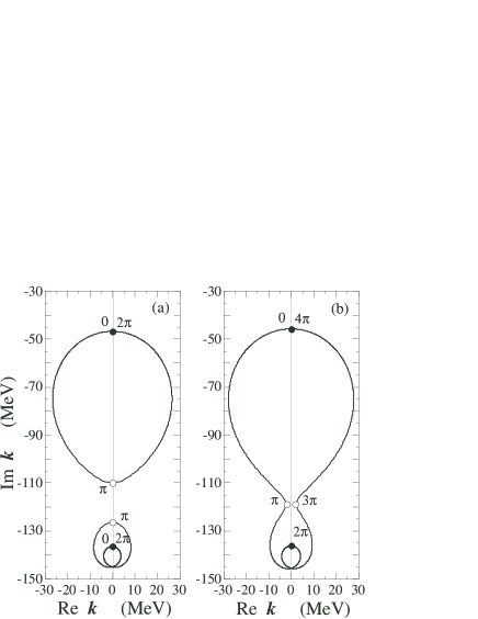
Figure 1: An example of fusion of two $2\pi$-periodic trajectories. (a) Before fusion, the upper trajectory is $(\mathrm{R}_{1}-\mathrm{A}_{1})$ and the lower trajectory is $(\mathrm{R}_{2}-\mathrm{A}_{2})$. Here $U$ is 4 MeV. (b) After fusion, the $4\pi$-periodic trajectory $(\mathrm{A}_{2}-\mathrm{A}_{1})$ is produced. Here the trajectory is shown at $U=4.2$ MeV. In these figures the closed circles indicate the locations of poles for the attractive sector, while the open circles for the repulsive sector.

The fusion occurs for $\phi=\pi$ on the negative imaginary momentum axis. An example of this process can be seen in Fig. 1 for $n=1$. In Fig. 1 (a) the upper trajectory is $({\mathrm{R}}_{1}-{\mathrm{A}}_{1})$ and the lower one is $({\mathrm{R}}_{2}-{\mathrm{A}}_{2})$ where the winding behavior noted above can be seen. In Fig. 1 (b) these two trajectories fuse into one trajectory $({\mathrm{A}}_{2}-{\mathrm{A}}_{1})$. Further increase of $U$ causes the replacement of $\mathrm{A}_{2}$ with $\mathrm{A}_{3}$ by a rearrangement processes given below.

III.2.2 Rearrangement

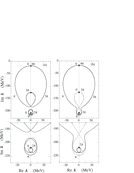
Figure 2: An example of rearrangement between a $2\pi$-periodic trajectory and a $4\pi$-periodic trajectory. (a) Before rearrangement, the upper trajectory is $(\mathrm{A}_{2}-\mathrm{A}_{1})$ and the lower trajectory is $(\mathrm{R}_{3}-\mathrm{A}_{3})$. The value of $U$ is 10.3 MeV. (b) After rearrangement, the upper trajectory is $(\mathrm{A}_{3}-\mathrm{A}_{1})$ (the solid curve) and the lower trajectory is $(\mathrm{R}_{3}-\mathrm{A}_{2})$ (the dashed curve). The value of $U$ is 10.5 MeV. We show below the enlarged figures around the contact points of two trajectories. The closed circles indicate the poles for the attractive sector of the potential, and the open circles for the repulsive sector.

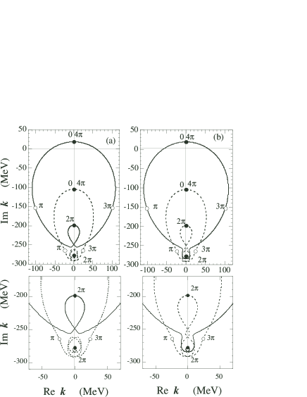
Figure 3: An example of rearrangement between two $4\pi$-periodic trajectories. (a) Before rearrangement, the upper trajectory is $(\mathrm{A}_{3}-\mathrm{A}_{1})$ (the solid curve) and the lower trajectory is $(\mathrm{A}_{4}-\mathrm{A}_{2})$ (the dashed curve). The value of $U$ is 20.4 MeV. (b) After rearrangement, the upper trajectory is $(\mathrm{A}_{4}-\mathrm{A}_{1})$ and the lower trajectory is $(\mathrm{A}_{3}-\mathrm{A}_{2})$. The $U$ is 20.5 MeV. Below are shown the enlarged parts of the figures around the contact points of two trajectories. The closed circles indicate the poles for the attractive sector of the potential, and the open circles for the repulsive sector.

There are two types of rearrangement process, (i) and (ii).

(i) Rearrangement between a $2\pi$-periodic trajectory and a $4\pi$-periodic trajectory,

$$({\mathrm{R}}_{m^{\prime}}-{\mathrm{A}}_{m}) + ({\mathrm{A}}_{n^{\prime}}-{\mathrm{A}}_{n})$$ (17)

$$\to ({\mathrm{R}}_{m^{\prime}}-{\mathrm{A}}_{n^{\prime}})+({\mathrm{A}}_{m}-{\mathrm{A}}_{n})\,$$

with $n<n^{\prime}<m\leq m^{\prime}$. In the process (i) there occurs exchange of trajectory segments including poles $\mathrm{A}_{m}$ and $\mathrm{A}_{n^{\prime}}$ between the two trajectories. The trajectory $({\mathrm{A}}_{n^{\prime}}-{\mathrm{A}}_{n})$ contacts the trajectory $({\mathrm{R}}_{m^{\prime}}-{\mathrm{A}}_{m})$ at $\alpha=\alpha_{\mathrm{c}}$ with $\pi<\alpha_{\mathrm{c}}<2\pi$ and its symmetric point at $\alpha=4\pi-\alpha_{\mathrm{c}}$, while the partner $2\pi$-periodic trajectory $({\mathrm{R}}_{m^{\prime}}-{\mathrm{A}}_{m})$ contacts at $\alpha_{\mathrm{c}}$ and at $\alpha=2\pi-\alpha_{\mathrm{c}}$ owing to the $2\pi$ periodicity of this trajectory. An example of the process (i) is given in Fig. 2 for $n=1,n^{\prime}=2,m=3,$ and $m^{\prime}=3$.

(ii) Rearrangement between two $4\pi$-periodic trajectories,

$$({\mathrm{A}}_{m^{\prime}}-{\mathrm{A}}_{m}) + ({\mathrm{A}}_{n^{\prime}}-{\mathrm{A}}_{n})$$ (18)

$$\to ({\mathrm{A}}_{n^{\prime}}-{\mathrm{A}}_{m})+({\mathrm{A}}_{m^{\prime}}-{\mathrm{A}}_{n})\,,$$

where we have the conditions $n<n^{\prime},m<m^{\prime},n<m,$ and $n^{\prime}<m^{\prime}$.

In the process (ii), the two trajectories contact at $\alpha=\alpha_{\mathrm{c^{\prime}}}$ with $\pi<\alpha_{\mathrm{c^{\prime}}}<2\pi$ and its symmetric point at $\alpha=4\pi-\alpha_{\mathrm{c^{\prime}}}$ where both trajectories develop somewhat protruded structures similar to those observed in Fig. 2. An example of the process (ii) is given in Fig. 3 for $n=1,n^{\prime}=3,m=2,$ and $m^{\prime}=4$.

III.3 Hulthén potential

The Hulthén potential htpt is given with $c=-1$ for Eq. (8) as

$$V_{0}(r)=-U\frac{\exp\left(-{r}/{r_{0}}\right)}{\Bigl{[}1-\exp\left(-{r}/{r_{0}}\right)\Bigr{]}}\,.$$ (19)

This is the only potential which is singular at $r=0$ in the class of Eckart potentials and produces no resonance and antiresonance poles for the repulsive sector. The Jost function is nwtn

$$f(k,\alpha)=\frac{\Gamma(1+2{i}kr_{0})}{\Gamma(1+{i}kr_{0}+D)\Gamma(1+{i}kr_{0}-D)}\,,$$ (20)

where $D$ is defined by $(g-k^{2}r_{0}^{2})^{1/2}$ with $g\equiv 2mr_{0}^{2}Ue^{i\alpha}$. If we use the infinite-product representation for the gamma function by Euler

$$\Gamma(z)=\frac{1}{z}\prod_{n=1}^{\infty}\biggl{[}\bigg{(}1+\frac{1}{n}\bigg{)}^{z}\bigg{(}1+\frac{z}{n}\bigg{)}^{-1}\biggr{]}\,,$$ (21)

the Jost function (20) is represented as

$$f(k,\alpha)=\prod_{n=1}^{\infty}\biggl{[}1-\frac{g}{n(n+2{i}kr_{0})}\biggr{]}\,.$$ (22)

The zeros of the Jost function $f(-k,\alpha)$ give the pole momentum

$$k_{n}(\alpha)={i}\frac{1}{2r_{0}}\left(\frac{2mr_{0}^{2}Ue^{i\alpha}}{n}-n\right)\,\qquad(n=1,2,\dots).$$ (23)

When $\alpha$ is zero, the moving poles appear on the positive imaginary axis for $n^{2}<g$ as the bound states, and on the negative imaginary axis for $n^{2}>g$ as the antibound states. The $S$-matrix has also an infinite number of fixed poles coming from the poles of the Jost function $f(k)$ on the positive imaginary axis, common to the class of Eckart potentials with exponential-tail.

Since the momentum of antibound-state or of a bound-state pole has an explicit expression in this case, it is easy to trace the pole with respect to $\alpha$. The trajectory is $(\mathrm{R}_{n}-\mathrm{A}_{n})$ with $n=1,2,\dots$ and is a circle having $2\pi$ periodicity with its center at $k_{n}^{\mathrm{FZ}}$ and radius $mr_{0}U/n$. All the pole trajectories of the Hulthén potential are stable without interfering with other trajectories for increase of $U$, though the crossing of $(R_{n}-A_{n})$ over $(R_{n^{\prime}}-A_{n^{\prime}})$ with $n<n^{\prime}$ occurs.

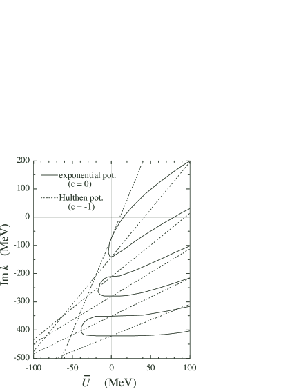
Figure 4: The behavior of moving poles of the exponential $(c=0)$ and the Hulthén $(c=-1)$potential for $\overline{U}\equiv e^{i\alpha}U$ on the imaginary momentum axis. The region $\overline{U}>0$ is the real attractive sector and the region with $\overline{U}<0$ is the repulsive one. The pole in the region Im $k>0$ is the bound state and the pole in the region Im $k<0$ is the antibound state.

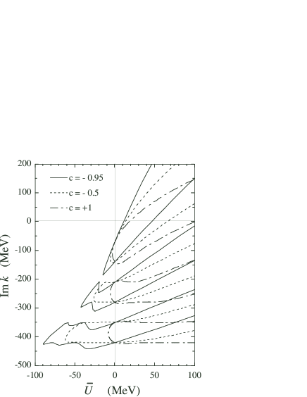
Figure 5: The behavior of moving poles of the generalized Hulthén potential for $c=1.0,-0.5,-0.95$ for $\overline{U}\equiv e^{i\alpha}U$ on the imaginary momentum axis. The region $\overline{U}>0$ is the real attractive sector and the region with $\overline{U}<0$ is the repulsive one. The pole in the region Im $k>0$ is the bound state and the pole in the region Im $k<0$ is the antibound state.

III.4 Formation of resonance poles by potentials with exponential-tail

Any trajectory of $4\pi$ periodicity involves a resonance and its conjugate antiresonance poles for the repulsive sector.

In the weak limit of the potential strength $U$, the spectrum of antibound-state poles takes the same pattern both for the exponential and the Hulthén potentials. If $U$ increases for the attractive sector ($e^{i\alpha}=+1$), these antibound-state poles move upward on the negative imaginary momentum axis, and finally appear as bound state poles on the positive imaginary axis in both potentials.

For the repulsive sector ($e^{i\alpha}=-1$), the movement of poles is different between these two potentials. In the Hulthén potential all the antibound-state poles move downward on the negative imaginary axis to $-i\infty$, while in the exponential potential the top antibound-state pole moves downward and the second moves upward, the third downward and the fourth upward, and so on. For $U$ continues to increase further, the top and the second collide and leave the imaginary momentum axis, becoming a pair of resonance and antiresonance poles. If $U$ increases further, the same happens for the third and the fourth antibound-state pole, and this continues. The pair of poles R_n and R_n+1 ($n=1,3,5,...$) become a resonance and its conjugate antiresonance.

The behavior of antibound-state poles is shown for the exponential and the Hulthén potential in Fig. 4 about six antibound-state poles starting from $k_{n}^{\mathrm{FZ}}$ ($n=1-6$) where the abscissa is the effective potential strength $\overline{U}\equiv e^{i\alpha}U$. As $\overline{U}$ decreases, the six straight dashed lines of the Hulthén potential go to $-\infty$ without mutual interference, while the six solid lines of the exponential potential go to the points of collision.

These features of the exponential potential are common to the potentials (8) with exponential tail with $c>-1$. The movement of antibound-state for the repulsive sector is monotone for the exponential, but as the potential leaves the exponential with $c$ different from zero, the poles move in somewhat complicated ways, but finally turn into resonance and antiresonance poles as in the exponential potential.

We show this for some cases of the generalized Hulthén potential In Fig. (5) where the results for $c=1,-0.5,$ and $-0.95$ are plotted. The collision between two poles is always “head-on” with one descending and the other ascending on the imaginary momentum axis. One might take the curves of $c=-0,5$ or $1$ as simple and smooth, differently from $c=-0.95$. A detailed inspection, however, shows small oscillatory behavior in these cases.

III.5 Square potential

The familiar square potential gives the pole spectrum very different from those of exponential-tail potentials. We take the spherical square potential given by

$$V_{0}(r)=\left\{\begin{array}[]{rcl}-U&&r\leq r_{0}\\ 0&&r>r_{0}\,,\end{array}\right.$$ (24)

where $U$ is a real positive constant.

Among potentials with finite range, the square potential is the only one known so far for which the Schrödinger equation can be solved analytically for all angular momentum state at an arbitrary energyqm .

The $S$-matrix element for the state with the angular momentum $l$ is given by

$$S_{l}(k,\alpha)=\frac{kj_{l}(Kr_{0})h_{l}^{(2)\,\prime}(kr_{0})-Kj_{l}^{\,\prime}(Kr_{0})h_{l}^{(2)}(kr_{0})}{-kj_{l}(Kr_{0})h_{l}^{(1)\,\prime}(kr_{0})+Kj_{l}^{\,\prime}(Kr_{0})h_{l}^{(1)}(kr_{0})}\,,$$ (25)

where $h_{l}^{(1)}$ and $h_{l}^{(2)}$ are the spherical Hankel functions given by the spherical Bessel functions $j_{l}$ and $n_{l}$ as $h_{l}^{(1)}=j_{l}+i\,n_{l}$ and $h_{l}^{(2)}=j_{l}-i\,n_{l}$ with $K\equiv[2m(E+Ue^{i\alpha})]^{1/2}$. In this case all the poles are moving poles and there is no fixed-pole singularity. Here we examine mainly the $s$-wave and give a brief summary for the $p$-wave.

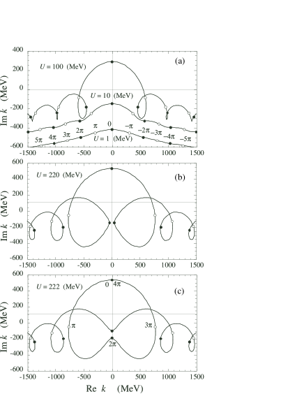
Figure 6: The change of the trajectory of the moving pole for $U$ where the closed circles indicates the locations of poles for the attractive potential, ($\alpha=0,\pm 2\pi,...$) while the open circles for the repulsive potential ($\alpha=\pm\pi,\pm 3\pi,...$). We attach the values of $\alpha$ to the curve of $U=1$ MeV in (a) and to those of $U=222$ MeV in (c).

III.5.1 The $s$-wave trajectories

The square potential produces a finite number of closed trajectories with $4\pi$ periodicity and one aperiodic open trajectory. For compactness, the term attractive is used for any pole of the real attractive sector of the potential and repulsive for the real repulsive sector.

If the potential strength $U$ is very small, there exists only one trajectory which is aperiodic one passing all the poles of real potentials; both attractive and repulsive resonance and anti-resonance poles as well as one attractive antibound-state pole for the change of phase $\phi$ from $-\infty$ to $+\infty$ with $\phi=0$ at the imaginary axis. The aperiodic open trajectory is special to the square potential.

The critical value $U_{0,{\rm cr}}^{n}$ of $U$ for the appearance of the $n$th $s$-wave bound state is

$$U_{0,{\rm cr}}^{n}=\frac{\pi^{2}}{8mr_{0}^{2}}(2n-1)^{2}\,\,\,\,(n=1,2,\dots)\,.$$ (26)

For $m=940$ MeV and $r_{0}=1/140$ (MeV)^-1 we have

$$U_{0,{\rm cr}}^{n}=25.7,\;231.5,\dots\,\,({\rm MeV})\,\,\,\,(n=1,2,\dots)\,.$$ (27)

When $U$ increases over the critical value $U_{0,{\mathrm{c}r}}^{1}$ for the appearance of the ground bound state, the antibound state becomes a bound state. As the potential strength increases further, the resonance pole with $\alpha=-2\pi$ and its conjugate antiresonance pole with $\alpha=+2\pi$ come close to and meet on the imaginary momentum axis, turning into two antibound-state poles. Then, one of these attractive antibound-state poles forms a $4\pi$-periodic trajectory with the ground bound-state pole together with a pair of repulsive resonance pole of $\alpha=-\pi$ and antiresonance pole of $\alpha=+\pi$, while the rest of the resonance and antiresonance poles forms an aperiodic trajectory passing the other attractive antibound-state pole.

These changes of the trajectories for $U$ are seen in Fig. 6. In Fig. 6(a) the real attractive and repulsive resonance and antiresonance poles lie on a simple smooth curve with one attractive antibound-state pole for $U=1$ MeV,

As $U$ increases, all the poles move upward, approaching (parting) the imaginary axis for $\alpha=\pm 2\pi.\pm 4\pi,...(\pm\pi,\pm 3\pi,...)$. For $U=100$ MeV there is one bound-state pole on the positive imaginary axis, which corresponds to the attractive antibound-state pole for $U=$ 1 and 10 MeV.

In Fig. 6(b) we give the trajectory for $U=220$ MeV, just before the formation of a closed loop from the aperiodic trajectory where a pair of resonance and antiresonace poles for $\alpha=\pm 2\pi$ appear near the negative imaginary momentum axis. In Fig. 6(c) we show the two trajectories at $U=222$ MeV, just after the formation of a closed loop trajectory with $4\pi$ periodicity from the aperiodic infinite trajectory. If $U$ increases further, the same process of the formation of a new closed trajectory repeats.

III.5.2 Notes on the $p$-wave trajectories

Since the square potential is the only known one for which we have the analytical solution of the $S$-matrix element for any angular momentum, it will be interesting to examine the trajectory structures of higher partial waves. Here we take the $p$-wave.

The basic structures of the $p$-wave trajectories can be considered as the same as the $s$-wave with one infinite trajectory and a finite number of closed trajectories for a finite value of $U$. There are, however, some differences in details. The formation process of the closed trajectory is somewhat complicated compared with the $s$-wave.

In the $s$-wave there appears one attractive antibound pole for very small $U$, while there exists only one repulsive antibound $p$-wave pole for an arbitrary value of $U$. The $p$-wave trajectory is an aperiodic trajectory relating all the poles including this repulsive antibound-state pole at $U$ smaller than the threshold value for the ground bound-state pole.

If $U$ increases, a pair of attractive resonance and antiresonance poles mutually approach and collide at the momentum $k=0$, then they turn into a bound-state pole and an antibound-state pole, which are the ground bound-state pole and the ground antibound-state pole, respectively. The ground bound-state lies on the aperiodic trajectories with the rest of resonance-antiresonance poles, and the ground antibound state pole forms a closed loop of $2\pi$ periodicity with the existing repulsive antibound-state pole.

Further increase of $U$ causes the contact between the aperiodic trajectory and the $2\pi$-periodic trajectory produces a $4\pi$-periodic trajectory passing the ground bound-state pole and the ground antibound-state pole as well as the nearest pair of repulsive resonance-antiresonace poles, while the repulsive antibound-state pole is on the aperiodic trajectory of remaining resonance and antiresonance poles.

This process of the formation of $4\pi$-periodic trajectory via the transient $2\pi$-periodic trajectory repeats each time as $U$ increases over a new threshold for excited bound-state pole. There the collision occurs between an attractive resonance and its conjugate antiresonance pole at $k=0$, giving new excited bound-state and antibound-state poles. It will be clear that any $4\pi$-periodic trajectory constitutes the bound-state and antibound-state poles simultaneously created by the collision. The $4\pi$-periodic trajectories, once there are produced, are stable for the increase of $U$ with no rearrangement with other trajectories, but the $2\pi$-periodic trajectory is an unstable intermediate product replacing its attractive antibound-state pole each time.

For angular momentum states higher than the $p$-wave, the basic pattern of formation of closed loops from an aperiodic trajectory is similar. There, however, appear different types of intermediate trajectories in the restructuring of trajectories. For example, we meet a pair of $2\pi$-periodic loops which are mutually conjugate partners and don’t cross the imaginary momentum axis. Trajectories of higher waves for the square potential will be discussed elsewhere.

IV Some Remarks

In this paper we have searched for some underlying structure of the quantum system by assuming a complex extension of real potentials. We have studied some global structure of the pole spectrum in the complex momentum plane. It has been found that the resonance-pole spectrum of the real repulsive potential plays the essential role for determining the trajectory structure. Most of potentials with exponential tail taken in this paper produce the resonance poles for the repulsive case as well as the square potential. The appearance of the $s$-wave resonances is not new, though seems to be discussed very seldom.

The most prevailing picture for the resonance formation in quantum mechanics will be that the resonance is produced by the attractive potential in collaboration with the centrifugal barrier. This explains the absence of the $s$-wave resonance state for attractive potentials except the square one. Such an intuitive interpretation is not available for the $s$-wave resonance which could be purely quantum mechanical effect, with no classical or semi-classical interpretations.

The appearance of resonance poles for the real square potentials, both attractive and repulsive, can be attributable to the singular nature of the potential edge. However, even the simple exponential potential produces repulsive resonance poles.

Although resonance poles appear near the real momentum axis of the physical region for some potentials with resonance-type effects, it is generally difficult to recognize the effects of $s$-wave resonances. The poles, however, influence the observables in the physical region, even if typical resonance-type effects are not produced. It seems necessary to exploit the implication of the $s$-wave resonance and its possible role in physics. If the repulsive $s$-wave resonance would be unphysical and should be removed, this would imposes a severe restriction on the plausible type of potentials.

In particle quantum mechanics there is practically no strong restriction for the potential. Except a few cases, most of potentials assumed in analyses of various processes are of phenomenological nature, taken for explaining the behavior of physical systems in some restricted area of the energy and the momentum transfer, and poles remote from the physical region of interest are not of serious concern. In quantum gauge field theories, the interactions among fields are built-in by the gauge symmetry as well as other invariance requirements qgft . The study of the quantum system with real potential in an extended framework as the present one might give some clue for this kind of problem.

All the moving poles have the same dynamical origin and we should pay more attention to the roles of all of the poles which characterize the physical system. The poles of the potentials with opposite signatures can be mutually related. This is one reason why we study a hyper system with complex potential $V(r)$ with $\alpha$ changing from $-\infty$ to $\infty$.

The physical and also mathematical implication of the topological structure of trajectory shown in this article is still to be clarified further. We hope that the present analysis will give a new aspect for deeper understanding of the quantum system.

*

Appendix A Trajectories near the fixed zeros for the exponential potential

As can be seen from Eq. (13), the bound-state and antibound-state poles come from the zeros of the Bessel function $J_{-i\nu}(\varphi)$. We are interested in how the zeros appear in the Bessel function. In order to consider the $n$th zero, we take the expansion of the Bessel function in terms of variable $v\equiv(\varphi/2)^{2}$,

$$J_{-i\nu}(\varphi)\,e^{i\nu/2} = \frac{1}{\Gamma(\epsilon+1-n)}-\frac{v}{1!\,\Gamma(\epsilon+2-n)}$$

$$+ \frac{v^{2}}{2!\,\Gamma(\epsilon+3-n)}-\frac{v^{3}}{3!\,\Gamma(\epsilon+4-n)}+\cdots\,.$$

where we make the substitution $i\nu\to n-\epsilon,\,\,\,(|\epsilon|<1)$.

If we take up to the $n$th term in the right-hand side of Eq. (A), the solution of $J_{-i\nu}(\varphi)=0$ is given by $\epsilon=0$ owing to the poles of the Gamma function, irrespectively of the value of $v$. This shows that we cannot terminate the expansion series at the $n$th term. We, therefore, have to take at least up to the $(n+1)$th term

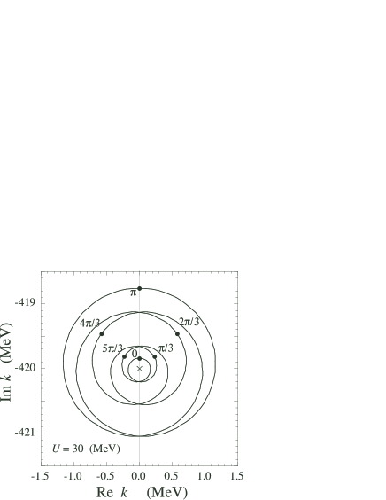
Figure 7: An example of winding behavior of the pole trajectory around the fixed zero for the exponential potential. This example is given for $n=6$ and $U=30$ MeV.

$$J_{-i\nu}(\varphi)\,e^{i\nu/2} = \frac{1}{\Gamma(\epsilon+1-n)}+\frac{(-v)}{1!\,\Gamma(\epsilon+2-n)}+\cdots$$ (29)

$$+\frac{1}{(n-1)!}\frac{(-v)^{n-1}}{\Gamma(\epsilon)}+\frac{1}{n!}\frac{(-v)^{n}}{\Gamma(\epsilon+1)}+\cdots$$

$$\approx \frac{1}{\Gamma(1+\epsilon)}\Bigl{\{}(\epsilon)_{n}+\frac{(-v)}{1!}(\epsilon)_{n-1}+\cdots$$

$$+\frac{(-v)^{n-1}}{(n-1)!}(\epsilon)_{1}+\frac{(-v)^{n}}{n!}\Bigr{\}}\,,$$

where the symbol $(\epsilon)_{j}\equiv\epsilon(\epsilon-1)\cdots(\epsilon-j+1)\,(j=1,2,...)$ is used.

The general solution of $\epsilon$ giving the zeros for the left-hand side of this equation will be hard to be obtained, but here we are interested in small $\epsilon$ as well as small $v$. We keep only the linear term in $\epsilon$ without $v$-dependent coefficient. This gives the solution for $\epsilon$ as

$$\epsilon=\frac{v^{n}}{n!(n-1)!}\,,$$ (30)

which vanishes only for $v=0$. Hence the trajectory $(\mathrm{R}_{n}-\mathrm{A}_{n})$ winds $n$-times around the point $k_{n}^{\mathrm{FZ}}$ for the change of $\alpha$ from zero to $2\pi$. As the potential strength $U$ increases, the contributions from higher order terms in $v$ become significant, but this winding feature remains strongly. An example is given in Fig. 7 for $n=6$ and $U=30$ MeV.

The winding property is critically dependent on the value of the parameter $c$ of the potential (8) as well as the potential strength $U$. In general the difference of the momentum $k(\alpha)$ of the antibound-state pole from the fixed zero, $k(\alpha)-k_{n}^{\mathrm{FZ}}$, starts linearly in $Ue^{i\alpha}$ for $c\neq 0$ and the winding number is one for very small $U$, while it behaves as $(Ue^{i\alpha})^{n}$ for $c=0$ . If $c$ is close to zero, higher terms in $U$ grow quickly as $U$ increases, inducing multiple-winding behavior.

References

- (1) H. Feshbach, C.E. Porter, and V. F. Weisskopf, Phys. Rev. 96, 448 (1954).
- (2) P. E. Hodgson, The Optical Model of Elastic Scattering (Clarendon Press, Oxford, 1963).
- (3) Some interesting recent development in this direction is the attempt of formulating the PT- invariant quantum mechanics. See for this, C.M. Bender, Rep. Prog. Phys. 70, 947 (2007) and references therein.
- (4) See N. Moiseyev, Phys. Rep. 302, 211 (1998); T. Andersen, Phys. Rep. 394, 157 (2004). The complex scaling method does not aim for complex extension of potentials directly, but concerns with non-hermitian potential in the process of complex scaling.
- (5) U.V. Riss and H.-D. Meyer, J. Phys. B 26, 4503 (1993); R. Lefebvre, M. Sindelka, and N. Moiseyev, Phys. Rev. A 72, 052704 (2005).
- (6) See, for example, V.I. Kukulin, V.M. Krasnopol’sky, and J. Horáček, Theory of Resonances; Principles and Applications (Kluwer Academic Pub., Dordrecht, Netherlands. 1989), Chap. 5.
- (7) Here we use the term resonance for all the poles with and .
- (8) For the original Hulthén potential, see L. Hulthén, Ark. Mat. Astron. Fys. A 28, 5 (1942). See also Ref. exppt .
-
(9)
R.G. Newton, Scattering Theory of Waves and Particles (Dover publications, Mineola, New York, 2002), pp. 421–422. The class of Eckart potentials is given by
- (10) M. Kawasaki, T. Maehara, and M. Yonezawa, arXiv: quant-ph/0810.3368v1, Mutual transformation among bound, virtual and resonance states in one-dimensional rectangular potentials.
- (11) For simple monotone potentials of definite signature, the definition of “attractive” or “repulsive” is obvious. As a generalization of this concept in the context of the present analysis, we may take a real potential as repulsive if no bound state is produced for scaling to by any positive value of , otherwise as attractive.
- (12) See, for example, A.G. Sitenko, Scattering Theory, Springer Series in Nuclear and Particle Physics (Springer-Verlag, BerlinHeidelberg, 1991), pp. 118–119.
- (13) See, for example, L.I. Schiff, Quantum Mechanics, 3rd ed. (McGraw-Hill, New York 1968), Sect.19.
- (14) See, for example, S. Weinberg, The Quantum Theory of Fields I, II (Cambridge University Press, 1996).