The effect of dipole-dipole interaction for two atoms with different couplings in non-Markovian environment

Abstract

Using the nonperturbative method, we study the exact entanglement dynamics of two two-level dipole-dipole interacting atoms coupled to a common non-Markovian reservoir with different coupling strengths. Besides analyzing the conditions for the existence of steady state, we find, though the dipole-dipole interaction could destroy the stationary entanglement, that relatively strong dipole-dipole interaction does suppress the disentanglement in the initial period of time. These results are helpful for the practical engineering of the entanglement in the future.

I Introduction

Quantum entanglement is highly relevant to the fundamental issues of quantum mechanics and plays a central role in the application of quantum information science. In recent years, the practical schemes for the creation of quantum entanglement have gained significant improvements both in theoretical research and in experimental realization. One of the most popular schemes involves a couple of spontaneously emitting two-level atoms (qubits) trapped in a single-mode cavity DDE1 ; DDE2 ; DDE3 , which describes both atoms or ions trapped in an electromagnetic cavity and circuit-QED setups. The corresponding investigations reach notable results on the dynamical evolution of the bipartite entanglement DDE4 ; F1 ; F2 ; PM3 and the steady states of the composite two-atom system DDE3 ; DDE4 ; DDE5 ; F2 ; PM3 .

Most of the previous studies base on an essential assumption that the coupling strengths of the two atoms to the cavity mode are equal DDE1 ; DDE4 , which is a good approximation for the atoms in microwave cavity. However, in optical cavity, the two atoms usually no longer possess the equivalent coupling strengths to the cavity mode F2 ; PM3 . In F2 , the case of different coupling constant is considered, but the dipole-dipole interaction is neglected in the very beginning, as in PM3 .

In this paper, we study the two two-level dipole-dipole interacting atoms in an optical cavity via a nonperturbative method PM1 ; PM2 ; PM3 , and focus on the asymptotic and transient entanglement dynamics of the composite two-atom system.

For stationary entanglement, when the dipole-dipole interaction exists and the coupling strengths of the two atoms to the cavity mode are different, the final state of the two-atom system will become completely separable and the bipartite entanglement will collapse to zero, which indicates that there is no decoherence-free subspace in this case DFS . This result holds under both the Makovian and non-Markovian treatment. Thus, we conclude that the memory effect resulted from the finite correlation time of the reservoir in non-Markovnian limit does not influence the asymptotic bipartite entanglement.

It is shown further, for transient entanglement, that strong dipole-dipole interaction can suppress the decoherence and disentanglement. However, when the strength of the dipole-dipole interaction and coupling strength of the atoms to the environment, which determines the memory effect, are in the same magnitude order, the dipole-dipole interaction accelerates the decoherence and disentanglement for some initial states.

Finally, by transforming the true mode Hamiltonian which is used at the start PM2 ; QO to the quasimode Hamiltonian PM2 which separates the memory effect and the damping effect of the reservoir explicitly, we present a concrete physical interpretation for all the results derived in this paper.

II Theoretical framework

Consider two two-level atoms with a common zero-temperature bosonic reservoir, and take their dipole-dipole interaction into account from the very beginning. Under the rotating wave approximation (RWA), the Hamiltonian of the composite two-atom system plus the reservoir is given by ($\hbar=1$) DDH0 ; DDH :

$$H=H_{0}+H_{{\mathop{int}}}+H_{dd},$$

with

$$H_{0}=\omega_{1}\sigma_{+}^{(1)}\sigma_{-}^{(1)}+\omega_{2}\sigma_{+}^{(2)}\sigma_{-}^{(2)}+\int_{-\infty}^{\infty}{d\omega_{k}\omega_{k}b^{\dagger}(\omega_{k})b(\omega_{k})},$$ (1)

$$H_{int}=(\alpha_{1}\sigma_{+}^{(1)}+\alpha_{2}\sigma_{+}^{(2)})\int_{-\infty}^{\infty}{d\omega_{k}g(\omega_{k})b(\omega_{k})}+{\rm h.c.},$$ (2)

$$H_{dd}=K(\sigma_{+}^{(1)}\sigma_{-}^{(2)}+\sigma_{+}^{(2)}\sigma_{-}^{(1)}).$$ (3)

Now, we use the true mode Hamiltonian. Here, $\sigma_{\pm}^{(j)}$ and $\omega_{j}$ are the inversion operators and transition frequency of the $j$th qubit ($j=1,2$), and $b(\omega_{k})$, $b^{\dagger}(\omega_{k})$ are the annihilation and creation operators of the field mode of the reservoir. The mode index $k$ contains several variables which are two orthogonal polarization indexes and the propagation vector $\vec{k}$. To measure the coupling strength of the atoms to the cavity mode determined by the atom’s relative position in the cavity, we introduce the dimensionless constant $\alpha_{j}$ PM3 . The static part of the dipole-dipole interaction is proportional to $K=[\vec{d}\cdot\vec{d}-3(\vec{d}\cdot\vec{r}_{12})(\vec{d}\cdot\vec{r}_{12})/r_{12}^{2}]r_{12}^{-3}$, where $\vec{r}_{12}=\vec{r}_{1}-\vec{r}_{2}$ is the relative position, $\vec{d}$ is the electric dipole moment of the atom.

For an initial state of the form

$$\left|{\psi(0)}\right\rangle=(c_{10}\left|e\right\rangle_{1}\left|g\right\rangle_{2}+c_{20}\left|g\right\rangle_{1}\left|e\right\rangle_{2})\left|0\right\rangle_{E},$$ (4)

since $[H,N]=0$, where $N=\int_{-\infty}^{\infty}{d\omega_{k}b^{\dagger}(\omega_{k})b(\omega_{k})}+\sigma_{+}^{(1)}\sigma_{-}^{(1)}+\sigma_{+}^{(2)}\sigma_{-}^{(2)}$, the time evolution of the total system is confined to the subspace spanned by the bases $\{\left|e\right\rangle_{1}\left|g\right\rangle_{2}\left|0\right\rangle_{E},\left|g\right\rangle_{1}\left|e\right\rangle_{2}\left|0\right\rangle_{E},\left|g\right\rangle_{1}\left|g\right\rangle_{2}\left|{1_{k}}\right\rangle_{E}\}$:

$$\left|{\psi(t)}\right\rangle = c_{1}(t)e^{-i\omega_{0}t}\left|e\right\rangle_{1}\left|g\right\rangle_{2}\left|0\right\rangle_{E}+c_{2}(t)e^{-i\omega_{0}t}\left|g\right\rangle_{1}\left|e\right\rangle_{2}\left|0\right\rangle_{E}$$ (5)

$$+\int_{-\infty}^{\infty}{d\omega_{k}c_{\omega_{k}}(t)e^{-i\omega_{k}t}\left|g\right\rangle_{1}\left|g\right\rangle_{2}\left|{1_{k}}\right\rangle}_{E},$$

where $\left|{1_{k}}\right\rangle_{E}$ is the state of the reservoir with only one exciton in the $k$th mode. Here, we consider the case in which the two atoms have the same frequency, i.e., $\omega_{1}=\omega_{2}=\omega_{0}$. According to the Schr$\rm\ddot{o}$dinger’s equation, the equations for the probability amplitudes take the form

$$i\dot{c}_{1}(t)=\alpha_{1}\int_{-\infty}^{\infty}{d\omega_{k}e^{-i(\omega_{k}-\omega_{0})t}g(\omega_{k})}c_{\omega_{k}}(t)+Kc_{2}(t),$$ (6)

$$i\dot{c}_{2}(t)=\alpha_{2}\int_{-\infty}^{\infty}{d\omega_{k}e^{-i(\omega_{k}-\omega_{0})t}g(\omega_{k})}c_{\omega_{k}}(t)+Kc_{1}(t),$$ (7)

$$i\dot{c}_{\omega_{k}}(t)=[{\alpha_{1}c_{1}(t)+\alpha_{2}c_{2}(t)}]g^{*}(\omega_{k})e^{i(\omega_{k}-\omega_{0})t}.$$ (8)

Eliminating the coefficients $c_{\omega_{k}}(t)$ by integrating Eq. (8) and substituting the result into Eqs. (6) and (7), we get:

$$\dot{c}_{1}(t)= - \int_{0}^{t}{dt_{1}f(t-t_{1})\alpha_{1}[\alpha_{1}c_{1}(t_{1})+\alpha_{2}c_{2}(t_{1})]}$$ (9)

$$- iKc_{2}(t),$$

$$\dot{c}_{2}(t)= - \int_{0}^{t}{dt_{1}f(t-t_{1})\alpha_{2}[\alpha_{1}c_{1}(t_{1})+\alpha_{2}c_{2}(t_{1})]}$$ (10)

$$- iKc_{1}(t),$$

where the responding function takes the form:

$$f(t-t_{1})=\int_{-\infty}^{\infty}{d\omega_{k}J(\omega_{k})}e^{-i(\omega_{k}-\omega_{0})(t-t_{1})}.$$

Suppose the atoms interacting resonantly with the reservoir with Lorentzian spectral density

$$J(\omega_{k})=\left|{g(\omega_{k})}\right|^{2}={W}^{2}\lambda/\pi[(\omega_{k}-\omega_{0})^{2}+\lambda^{2}],$$

by employing Fourier transform and residue theorem, we get the explicit form $f(t-t_{1})={W}^{2}e^{-\lambda(t-t_{1})}$, where the quantity $1/\lambda$ is the reservoir correlation time.

In fact, we can obtain the solution by Laplace approach directly. However, in order to construct a lucid physical insight, we choose the pseudo-mode approach PM1 ; PM2 ; PM3 . The corresponding equations are as follows:

$$\dot{c}_{1}(t)=-iW\alpha_{1}b(t)-iKc_{2}(t),$$ (11)

$$\dot{c}_{2}(t)=-iW\alpha_{2}b(t)-iKc_{1}(t),$$ (12)

$$\dot{b}(t)=-\lambda b(t)-iW[\alpha_{1}c_{1}(t_{1})+\alpha_{2}c_{2}(t_{1})],$$ (13)

where

$$b(t)=-i\int_{0}^{t}{dt_{1}e^{-\lambda(t-t_{1})}W[\alpha_{1}c_{1}(t_{1})+\alpha_{2}c_{2}(t_{1})]},$$

Taking Laplace transform, $c_{1,2}(t)\fallingdotseq\bar{c}_{1,2}(s),\ b(t)\fallingdotseq\bar{b}(s)$, we get the resulting equations

$$s\bar{c}_{1}(s)-c_{10}=-iW\alpha_{1}\bar{b}(s)-iK\bar{c}_{2}(s),$$ (14)

$$s\bar{c}_{2}(s)-c_{20}=-iW\alpha_{2}\bar{b}(s)-iK\bar{c}_{1}(s),$$ (15)

$$s\bar{b}(s)-b(0)=-\lambda\bar{b}(s)-iW[\alpha_{1}\bar{c}_{1}(s)+\alpha_{2}\bar{c}_{2}(s)].$$ (16)

Further, we introduce vacuum Rabi frequency $R=W(\alpha_{1}^{2}+\alpha_{2}^{2})^{1/2}$ and relative coupling strengthes $r_{j}=\alpha_{j}(\alpha_{1}^{2}+\alpha_{2}^{2})^{-1/2}$ ($j=1,2$). Applying the inverse Laplace transform, we get the solutions with the initial condition $b(0)=0$:

$$c_{1}(t)=\sum\limits_{s_{i}}{\mathop{\lim}\limits_{s\to s_{i}}\left\{{(s-s_{i})\frac{{c_{10}[s(s+\lambda)+R^{2}r_{2}^{2}]-c_{20}[iK(s+\lambda)+R^{\rm{2}}r_{1}r_{2}]}}{{s^{2}(s+\lambda)+R^{2}s+K^{2}(s+\lambda)-2iKR^{2}r_{1}r_{2}}}}\right\}}e^{s_{i}t},$$ (17)

$$c_{2}(t)=\sum\limits_{s_{i}}{\mathop{\lim}\limits_{s\to s_{i}}\left\{{(s-s_{i})\frac{{c_{20}[s(s+\lambda)+R^{2}r_{1}^{2}]-c_{10}[iK(s+\lambda)+R^{2}r_{1}r_{2}]}}{{s^{2}(s+\lambda)+R^{2}s+K^{2}(s+\lambda)-2iKR^{2}r_{1}r_{2}}}}\right\}}e^{s_{i}t},$$ (18)

$$b(t)=-iR\sum\limits_{s_{i}}{\mathop{\lim}\limits_{s\to s_{i}}\left\{{(s-s_{i})\frac{{(r_{1}c_{10}+r_{2}c_{20})s-iK(r_{1}c_{20}+r_{2}c_{10})}}{{s^{2}(s+\lambda)+R^{2}s+K^{2}(s+\lambda)-2iKR^{2}r_{1}r_{2}}}}\right\}}e^{s_{i}t}.$$ (19)

where $s_{i}$ belongs to the roots of the following equation for $s$:

$${s^{2}(s+\lambda)+R^{2}s+K^{2}(s+\lambda)-2iKR^{2}r_{1}r_{2}}=0.$$ (20)

Asymptotic analysis.—In physical problems considered in this paper, $\bar{c}_{1,2}(s)$ have poles which lie either on the imaginary axis, giving an oscillatory term, or in the left-hand half plane, giving a term which exponentially decays in magnitude. Consider function $\bar{c}_{1,2}(s)$ each having a single simple pole $s_{0}=i\theta$ lying on the imaginary axis, and all other poles lying in the left-hand half plane. The residue at $s_{0}=i\theta$ is

$$\mathop{\lim}\limits_{s\to i\theta}(s-i\theta)\bar{c}_{1,2}(s)\exp(i\theta t).$$ (21)

The other residues are of the form ${\mathop{\lim}\limits_{s\to s_{i}}h_{i}\exp(s_{i}t)}$, where $h_{i}$ is a constant determined by $s_{i}$. Since each $s_{i}$ has a negative real part, the residue decays exponentially in magnitude as $t$ increases. So, whether the values of $c_{1}$ and $c_{2}$ are zero as $t\rightarrow\infty$ depends on wether Eq. (20) has a pure imaginary solution. Hence, it is easy to figure out that the conditions for the existence of the steady state are

$$K=0\ \rm{or}\ \alpha_{1}=\alpha_{2},$$ (22)

which means unless there is no dipole-dipole interaction or the coupling strengths of the two atoms to the cavity mode are equal, $c_{1}(t)$ and $c_{2}(t)$ will tend to be zero as $t\rightarrow\infty$.

In the $\{\left|e\right\rangle_{1}\left|e\right\rangle_{2},\left|e\right\rangle_{1}\left|g\right\rangle_{2},\left|g\right\rangle_{1}\left|e\right\rangle_{2},\left|g\right\rangle_{1}\left|g\right\rangle_{2}\}$ basis, the reduced density matrix of the two atoms is given by:

$$\rho_{a}(t)=\left({\begin{array}[]{*{20}c}0&0&0&0\\ 0&{\left|{c_{1}(t)}\right|^{2}}&{c_{1}(t)c_{2}^{*}(t)}&0\\ 0&{c_{2}(t)c_{1}^{*}(t)}&{\left|{c_{2}(t)}\right|^{2}}&0\\ 0&0&0&{1-\left|{c_{1}(t)}\right|^{2}-\left|{c_{2}(t)}\right|^{2}}\\ \end{array}}\right).$$ (23)

We choose the concurrence $C(t)$ Concurrence to measure the entanglement of the two atoms. According to the definition, the expression of the concurrence of $\rho_{a}$ is given by Concurrence :

$$C(t)=2\left|{c_{1}(t)c_{2}^{*}(t)}\right|=2\left|{c_{1}(t)}\right|\left|{c_{2}(t)}\right|.$$ (24)

First, consider $\alpha_{1}=\alpha_{2}$, that is, the coupling constants of the two atoms to the cavity mode are the same. The asymptotic entanglement evaluated by the concurrence is given by:

$$C(t\to\infty)=\left|{c_{10}-c_{20}}\right|^{2}/2.$$

This indicates that stationary entanglement is only determined by the initial state of the system.

Next, consider $K=0$, that is, the dipole-dipole interaction is neglected. The asymptotic entanglement is given by

$$C(t\to\infty)=2\left|{\alpha_{R}^{-1}c_{10}-c_{20}}\right|\left|{\alpha_{R}c_{20}-c_{10}}\right|/(\alpha_{R}^{2}+\alpha_{R}^{-2}),$$

where $\alpha_{R}=r_{1}/r_{2}$. This indicates that the entanglement is determined by the initial state and the ratio of the coupling constants of the two atoms to the cavity mode. This situation has been discussed in details in PM3 .

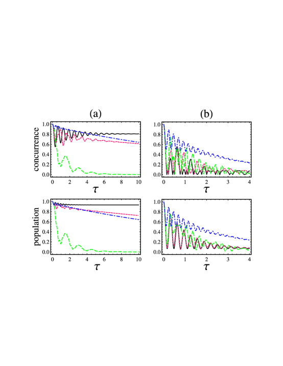
Figure 1: (color online) Time evolution of the concurrence and population, with the initial state being (a) $\left|{\varphi_{-}}\right\rangle$, and (b) $\left|{\varphi_{+}}\right\rangle$, both with $R=10$, $\lambda=1$ and $r_{1}=\sqrt{3}/2$, for the cases of (i) no dipole-diploe interaction ${\cal K}=0$ (solid curve), (ii) weak dipole-dipole interaction ${\cal K}=2$ (short-dashed curve), (iii) intermediate dipole-dipole interaction ${\cal K}=7$ (long-dashed curve), and (iv) strong dipole-dipole interaction ${\cal K}=20$ (long-short-dashed curve).

Dynamical analysis.—In this part, we will focus on the entanglement dynamical evolution of the composite system in a good cavity, i.e., for $\cal R\rightarrow\infty$ with ${\cal R}=R/\lambda$. In FIG. 1, we show the concurrence as a function of $\tau=\lambda t$ in the good cavity limit. We compare the dynamics of two maximally entangled states (MES: $\left|{\varphi_{\pm}}\right\rangle$) for four different values of relative strengths of dipole-dipole interaction, namely, ${\cal K}=0,2,7,20$, with ${\cal K}=K/\lambda$ which represents the ratio of the strength of the dipole-dipole interaction to the coupling strength of the atoms to the cavity field. The explicit expressions of $\left|{\varphi_{-}}\right\rangle$ and $\left|{\varphi_{+}}\right\rangle$ are as follows:

$$\left|{\varphi_{\pm}}\right\rangle=\frac{1}{{\sqrt{2}}}(\left|e\right\rangle_{1}\left|g\right\rangle_{2}\pm\left|g\right\rangle_{1}\left|e\right\rangle_{2}).$$ (25)

We choose the coupling parameter $r_{1}$ as $\sqrt{3}/2$, which is a typical constant in our case. Other values of $r_{1}$ which exclude $r_{1}=1/\sqrt{2}$ show qualitatively similar behavior. Here, We note that when $r_{1}=r_{2}=1/\sqrt{2}$, $\left|{\varphi_{-}}\right\rangle$ spans an eigenspace of the Hamiltonian of the composite system with and without dipole-dipole interaction, which means that once the initial state is $\left|{\varphi_{-}}\right\rangle$, both the population and concurrence will stay at their maximal value 1 as time increases irrespective of what the relative strength $\cal K$ is.

For a MES $\left|{\varphi_{-}}\right\rangle$, and for the case of ${\cal K}=0$, the population and concurrence oscillate at the very beginning, but as time increases the composite two-atom system collapses to a steady state, which means that the black plots for both the population and concurrence will converge to a straight line with a fixed value as $\tau$ increases. However, when we take into account the dipole-dipole interaction (${\cal K}\neq 0$) with $r_{1}\neq r_{2}$, both the population and concurrence perform damped oscillations and tend to be zero inevitably as time increases which means that the composite system has no steady state and will lose their bipartite entanglement completely just as our asymptotic analysis describes. When ${\cal K}=2$, the entanglement collapses faster with the growing strength of the dipole-dipole interaction. On the contrary, when ${\cal K}=20$, the entanglement collapses more slowly with the increasing strength of the dipole-dipole interaction. The fastest disentanglement happens when the strength of dipole-dipole interaction and the coupling strength of the atoms to the cavity field are in the same order of magnitude (${\cal K}\approx 7$), given all other conditions the same, as shown in FIG. 1 (a). Whereas, for a MES $\left|{\varphi_{+}}\right\rangle$, the disentanglement becomes slower as the dipole-dipole interaction become stronger, which means the dipole-dipole interaction can inhibit decoherence and disentanglement, as shown in FIG. 1 (b). In the practical engineering of entanglement, this result suggest that if it is hard to gain equal couplings between the atoms to the cavity, one can simply choose an appropriate distance to make the couplings of the atoms to the cavity to be much smaller or bigger than the dipole-dipole interactions. This will, at least, keep the entanglement alive for a longer time.

In FIG. 1, we choose $\lambda/W=0.1$, which can be well realized within the current experimental condition ECQED . A more intuitive impression of the role of the dipole-dipole interaction can be get from FIG. 2. The explanations of these results will be given in details in the following section.

III Explanations by quasimode Hamiltonian

In order to erect a concrete explanation for these phenomena, we convert the true mode Hamiltonian with Lorentz spectral density into the quasimode form, because in the truemode Hamiltonian, the coupling between the atoms and infinite modes makes it hard to separate the damping effect and the memory effect. Using the method in PM2 , we get:

$$H=H_{0}^{\prime}+H_{int}^{\prime}+H_{dd}+H_{damping},$$ (26)

$$H_{0}^{\prime} = \omega_{1}\sigma_{+}^{(1)}\sigma_{-}^{(1)}+\omega_{2}\sigma_{+}^{(2)}\sigma_{-}^{(2)}+\omega_{0}a^{\dagger}a$$ (27)

$$+\int_{-\infty}^{\infty}{d\Delta\Delta c^{\dagger}(\Delta)c(\Delta)},$$

$$H_{int}^{\prime}=W[(\alpha_{1}\sigma_{+}^{(1)}+\alpha_{2}\sigma_{+}^{(2)})a+(\alpha_{1}\sigma_{-}^{(1)}+\alpha_{2}\sigma_{-}^{(2)})a^{\dagger}],$$ (28)

$$H_{damping}=(\lambda/\pi)^{1/2}\int_{-\infty}^{\infty}{d\Delta[a^{\dagger}c(\Delta)+ac^{\dagger}(\Delta)]},$$ (29)

where $c^{\dagger}(\Delta),c(\Delta)$ are the creation and annihilation operators of the continuum quasimode of frequency $\Delta$, $H_{dd}$ and the other parameters are the same as before.

From the above Hamiltonian, the composite two-atom system only interacts with one discrete mode and their coupling coefficients are just the transition strength $\alpha_{i}W$ ($i=1,2$). The discrete mode interacts with a set of continuum modes PM2 and their coupling strength only contains the width of the Lorentzian spectral density $\lambda$ which is a constant. This means that if we let the two atoms and the discrete mode be a new system and the continuum modes be the reservoir, the behavior of the new system is exactly Markovian. The physical interpretation of the quasimode Hamiltonian has been discussed in details in PM2 , and more details about the relations between the quasimode and the true mode Hamiltonian are given in the appendix. Now we use the quasimode Hamiltonian to explain the results derived above.

The first thing is the origin of the Non-Markovian memory effect. As we know, the memory effect originates from the finite lifetime of the photon in the cavity PM2 ; PM3 . According to Eqs. (26)-(29), the atoms only interact with the discrete mode, while the irreversible process only happens in the interaction between the discrete mode and the continuum modes. So, the reabsorbing phenomenon that causes the entanglement to oscillate, as shown in FIG. 1, just results from the interaction between the atoms and the discrete mode, which is a reversible process. Yet, due to the coupling between the discrete and the continuum modes, the photon escapes into the continuum modes and never comes back, for the process is exactly Markovian. This means that the memory effect is a finite time phenomenon, which fits the results in FIG. 1 where the oscillating phenomenon is only obvious at the very beginning.

The second thing is the disentanglement suppressing effect in the strong dipole-dipole interaction. From Eqs. (26)-(29), we can see that the atoms are only coupled to the discrete mode, while the damping process only happens between the discrete and the continuum modes. This indicates that if the exciton only exists in the atoms, the damping process does not happen. The damping of the atoms happens only when the exciton in the atomic system is transferred to the discrete mode by the interaction between them and then photon escapes to the continuum modes before it comes back to the atomic system again. That is to say, the probability of the exciton transferring from the atom to the discrete mode is related to the disentanglement. As shown in FIG. 2, if the dipole-dipole interaction is much stronger than the interaction between the atom and the discrete quasimode, the disentanglement happens very slowly. So, in terms of quantum perturbation theory, the dynamics of the atoms is mainly determined by $H_{dd}$. Because the initial state $\left|{\varphi_{-}}\right\rangle$ form an invariant subspace of $H_{dd}$, the atoms will stay in this state forever in the zeroth order perturbation consideration, and the disentanglement is caused only by the higher-order corrections, which are relatively small quantities. Therefore, the disentanglement happens slowly. However, when the two strengths are in the same order of magnitude, $H_{int}$ is not small quantity compared to $H_{dd}$, and the higher-order correction can not be treated as perturbation, and thus the disentanglement happens very fast. The analogous discussion goes well also for the case of the strength of dipole-dipole interaction $K$ being much smaller than the strength of the interaction between the atom and the discrete quasimode $W$.

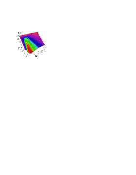
Figure 2: (color online) Time evolution of concurrence as a function of dipole-dipole interaction strength $K$, for the initial state $\left|{\varphi_{-}}\right\rangle$ with $R=10$, $\lambda=1$ and $r_{1}=\sqrt{3}/2$.

IV conclusion

In this paper, we extend the study of the entanglement dynamics to a realistic situation where the dipole-dipole interaction is not neglected and the couplings of the atoms to the field are different. We find, in this situation, that there is no steady state entanglement. This result is valid for both the Markovian and non-Markovian environment. Nevertheless, though the dipole-dipole interaction could destroy the asymptotic entanglement, strong dipole-dipole interaction does suppress disentanglement effect under some conditions. These results are helpful for the practical engineering of the entanglement in the future.

APPENDIX:  THE RELATIONS BETWEEN THE QUASIMODE HAMILTONIAN AND THE TRUE MODE HAMILTONIAN

The transform relation from the true mode Hamiltonian to the quasimode Hamiltonian is given by:

$$b(\omega_{k}) = \frac{{(\lambda/\pi)^{1/2}}}{{(\omega-\omega_{0})+i\lambda}}[a+(\lambda/\pi)^{1/2}{\rm P}\int_{-\infty}^{\infty}{d\Delta\frac{{c^{\dagger}(\Delta)}}{{\omega-\Delta}}}$$ (30)

$$+\frac{{\omega-\omega_{0}}}{{(\lambda/\pi)^{1/2}}}\int_{-\infty}^{\infty}{d\Delta c^{\dagger}(\Delta)}].$$

The transform relation from the quasimode Hamiltonian to the true mode Hamiltonian is given by:

$$a=(\lambda/\pi)^{1/2}\int_{-\infty}^{\infty}{d\omega_{k}\frac{{b(\omega_{k})}}{{\omega_{k}-\omega_{0}-i\lambda}}},$$ (31)

$$c(\Delta) = (\lambda/\pi){\rm P}\int_{-\infty}^{\infty}{d\omega_{k}\frac{{b(\omega_{k})}}{{(\omega_{k}-\Delta)(\omega_{k}-\omega_{0}-i\lambda)}}}$$ (32)

$$+\int_{-\infty}^{\infty}{d\omega_{k}\frac{{\omega_{k}-\omega_{0}}}{{\omega_{k}-\omega_{0}-i\lambda}}b(\omega)},$$

Using the quasimode Hamiltonian, the initial state is given by: $\left|{\psi(0)}\right\rangle{\rm{=}}c_{10}\left|e\right\rangle_{1}\left|g\right\rangle_{2}\left|0\right\rangle_{a}\mathop{\otimes}\limits_{\omega}\left|{0_{\omega}}\right\rangle-c_{20}\left|e\right\rangle_{1}\left|g\right\rangle_{2}\left|0\right\rangle_{a}\mathop{\otimes}\limits_{\omega}\left|{0_{\omega}}\right\rangle$. Since $[N,H]=0$, where $N=\sigma_{+}^{(1)}\sigma_{-}^{(1)}+\sigma_{+}^{(2)}\sigma_{-}^{(2)}+a^{\dagger}a+\int_{-\infty}^{\infty}{d\Delta c^{\dagger}(\Delta)c(\Delta)}$, we can write the state of the total system as

$$\left|{\psi(t)}\right\rangle = c_{1}(t)\left|e\right\rangle_{1}\left|g\right\rangle_{2}\left|0\right\rangle_{a}\mathop{\otimes}\limits_{\omega}\left|{0_{\omega}}\right\rangle+c_{2}(t)\left|g\right\rangle_{1}\left|e\right\rangle_{2}\left|0\right\rangle_{a}\mathop{\otimes}\limits_{\omega}\left|{0_{\omega}}\right\rangle$$ (33)

$$+ b(t)\left|g\right\rangle_{1}\left|g\right\rangle_{2}\left|1\right\rangle_{a}\mathop{\otimes}\limits_{\omega}\left|{0_{\omega}}\right\rangle$$

$$+ \int_{-\infty}^{\infty}{d\omega c(\omega)\left|g\right\rangle_{1}\left|g\right\rangle_{2}\left|0\right\rangle_{a}\left|{1_{\omega}}\right\rangle}.$$

According to Schr$\rm\ddot{o}$dinger’s equation, we find that the equations for $c_{1}(t)$, $c_{2}(t)$, and $b(t)$ are just the same as Eqs. (11), (12), and (13). This indicates that the pseudomode is just the discrete quasimode in the situation of Lorentzian spectral density.

References

• (1) Shi-Biao Zheng and Guang-Can Guo, Phys. Rev. Lett. 85, 2392 (2000).
• (2) S. Osnaghi et al., Phys. Rev. Lett. 87, 037902 (2001).
• (3) E. Hagley et al., Phys. Rev. Lett. 79, 1 (1997).
• (4) S. Nicolosi et al., Phys. Rev. A 70, 022511 (2004).
• (5) Z. Ficek and R. Tana$\rm{\acute{s}}$, Phys. Rev. A 74, 024304 (2006).
• (6) Sonny Natali and Z. Ficek, Phys. Rev. A 74, 042307 (2007).
• (7) Sabrina Maniscalco et al., Phys. Rev. Lett. 100, 090503 (2008).
• (8) P. Zanardi and M. Rasetti, Phys. Rev. Lett. 79, 3306 (1997); P. Zanardi, Phys. Rev. A 56, 4445 (1997).
• (9) B. M. Garraway, Phys. Rev. A 55, 2290 (1997).
• (10) B. J. Dalton et al., Phys. Rev. A 64, 053813 (2001).
• (11) A. Beige, Phys. Rev. A 67, 020301 (R) (2003).
• (12) O S. M. Barnett and P. M. Radmore, Methods in Theoretical Quantum Optics (Oxford University, Oxford, 1997).
• (13) G. S. Agarwal, Quantum Statistical Theories of Spontaneous Emission and Their Relation to Other Approaches (Springer-Verlag, 1974).
• (14) F. Seminara and C. Leonardi, Phys. Rev. A 42, 5695 (1990).
• (15) W. K. Wootters, Phys. Rev. Lett. 80, 2245 (1998).
• (16) S. Kuhr et al., Appl. Phys. Lett. 90, 164101 (2007).