Berry Phase in a Single Quantum Dot with Spin-Orbit Interaction

Abstract

Berry phase in a single quantum dot with Rashba spin-orbit coupling is investigated theoretically. Berry phases as functions of magnetic field strength, dot size, spin-orbit coupling and photon-spin coupling constants are evaluated. It is shown that the Berry phase will alter dramatically from $0$ to $2\pi$ as the magnetic field strength increases. The threshold of magnetic field depends on the dot size and the spin-orbit coupling constant.

I Introduction

Due to its important role in encoding information, the phase of wavefunction attracts a lot of interest in information science. Those properties can also be used in future quantum information and quantum computer. Thus selecting one kind of phases which can be manipulated by quantum effect is very important. Berry phase is believed to be a promising candidate. As a quantum mechanical system evolves cyclically in time such that it return to its initial physical state, its wavefunction can acquire a geometric phase factor in addition to the familiar dynamic phaseSegao ; Anandan . If the cyclic change of the system is adiabatic, this additional factor is known as Berry’s phaseBerry , and is, in contrast to dynamic phase, independent of energy and time. Fuentes-Guridi et al.Fuentes calculated the Berry phase of a particle in a magnetic field in consideration of the quantum nature of the light field. Yi et al.Yi studied the Berry phase in a composite system and showed how the Berry phases depend on the coupling between the two subsystems. In a recent paper, San-Jose et al.San have described the effect of geometric phases induced by either classical or quantum electric fields acting on single electron spins in quantum dots. Wang and Zhu Wang H. have investigated the voltage-controlled Berry phases in two vertically coupled InGaAs/GaAs quantum dots. Most recently, observations of Berry phases in solid state materials are reportedYuanbo ; Vartiainen ; Leek . Leek et al.Leek demonstrated the controlled Berry phase in a superconducting qubit which manipulates the qubit geometrically using microwave radiation and observes the phase in an interference experiment.

Spin-related effects have potential applications in semiconductor devices and in quantum computation. Rashba et al.Rashba have described the orbital mechanisms of electron-spin manipulation by an electric field. SoninSonin has demonstrated that an equilibrium spin current in a 2D electron gas with Rashba spin-orbit interaction can result in a mechanical torque on a substrate near an edge of the medium. SerebrennikovSerebrennikov considered that the coherent transport properties of a charge carrier. The transportation will cause a spin precession in zero magnetic fields and can be described in purely geometric terms as a consequence of the corresponding holonomy.

The spin-orbit interaction in semiconductor heterstructures is increasingly coming to be seen as a tool which can manipulate electronic spin states Egues ; Efros . Two basic mechanisms of the spin-orbit coupling of 2D electrons are directly related to the symmetry properties of QDs. They stem from the structure inversion asymmetry mechanism described by the Rashba termRashba ; Bychkov and the bulk inversion asymmetry mechanism described by the Dresselhaus termDresselhaus . Recently, Debald and Emary Debald have investigated a spin-orbit driven Rabi oscillation in a single quantum dot with Rashba spin-orbit coupling. However, the influence of spin-orbit interaction on Berry phase in a single quantum dot is still lacking. In the present paper we will give a detail study on the Berry phase evolution of a single quantum dot with spin-orbit interaction in a time-dependent quantized electromagnetic environment. We will borrow quantum optics method to investigate the impact of the spin-orbit interaction and spin-photon interaction on Berry phase.

The paper is organized as follows. In Sec.II, we give the model Hamiltonian including both spin-orbit interaction and spin-photon interaction and calculated Berry phases as functions of magnetic field strength, dot size, spin-orbit coupling and photon-spin coupling constants. In Sec.III, we draw the figures of the Berry phase as a function of magnetic field strength and some discussions are given. The final conclusion is presented in Sec.IV.

II Theory

We consider a simple two-dimensional quantum dot with parabolic lateral confinement potential in a perpendicular magnetic field $\bf{B}$ which points along $z$ direction. Then the electron system can be described by the Hamiltonian Debald ,

$${H_{s}}=\frac{(\textbf{p}+\frac{e}{c}\textbf{A})^{2}}{2m^{*}}+\frac{m^{*}}{2}\omega^{2}_{0}(x^{2}+y^{2})+\frac{1}{2}g\mu_{B}B\sigma_{z},$$ (1)

where p is the linear momentum operator of the electron, $\textbf{A}(\textbf{r})=\frac{\textbf{B}}{2}(-y,x,0)$ is the vector potential in the symmetric gauge, $\omega_{0}$ is the characteristic confinement frequency, and $\sigma=(\sigma_{x},\sigma_{y},\sigma_{z})$ is the vector Pauli matrices. $m^{*}$ is the effective mass of the electron and $g$ its gyromagnetic factor. $\mu_{B}$ is the Bohr magneton. In the second quantized notation, Eq.(1) becomes

$${H_{s}}=(a_{x}^{+}a_{x}+a_{y}^{+}a_{y}+1)\hbar\widetilde{\omega}+\frac{\hbar\omega_{c}}{2i}(a_{x}^{+}a_{y}-a_{x}a_{y}^{+})$$

$$+\frac{1}{2}g\mu_{B}B\sigma_{z},$$ (2)

where $\omega_{c}=\frac{eB}{m^{*}c}$ and $\widetilde{\omega}^{2}=\omega_{0}^{2}+\frac{\omega_{c}^{2}}{4}$. If we set

$$a_{+}=\frac{1}{\sqrt{2}}(a_{x}-ia_{y}),a_{-}=\frac{1}{\sqrt{2}}(a_{x}+ia_{y}),$$ (3)

Then, the Hamiltonian (2) can be written as

$${H_{s}}=n_{+}\hbar\omega_{+}+n_{-}\hbar\omega_{-}+\frac{1}{2}g\mu_{B}B\sigma_{z},$$ (4)

where $\omega_{\pm}=\widetilde{\omega}\pm\omega_{c}/2$, $n_{+}=a_{+}^{+}a_{+}$ and $n_{-}=a_{-}^{+}a_{-}$. In what follows we include the spin-orbit interaction which is described as Rashba Hamiltonian in this system Rashba

$${H_{so}}=-\frac{\alpha}{\hbar}[(\textbf{p}+\frac{e}{c}\textbf{A})\times\sigma]_{\it z},$$ (5)

where $\alpha$ is the spin-orbit coupling constant which can be controlled by gate voltage in experiment. On substituting Eq.(3) into Eq.(5) and then

$${H_{so}}=\frac{\alpha}{\widetilde{l}}[\gamma_{+}(\sigma_{+}a_{+}+\sigma_{-}a_{+}^{+})-\gamma_{-}(\sigma_{-}a_{-}+\sigma_{+}a_{-}^{+})],$$ (6)

where $\gamma_{\pm}=1\pm\frac{1}{2}(\widetilde{l}/l_{B})^{2}$, $\widetilde{l}=({\hbar}/{m^{*}\widetilde{\omega}})^{\frac{1}{2}}$ and $l_{B}=({\hbar}/{m^{*}\omega_{c}})^{\frac{1}{2}}$.

The Hamiltonians of photons and the coupling to the electron spin can be written as follows:

$$H_{p}=\hbar\omega_{p}b^{+}b,$$ (7)

$$H_{p-s}=g_{c}(\sigma_{+}+\sigma_{-})(b^{\dagger}+b),$$ (8)

where $b^{+}$ ($b$) and $\omega_{p}$ are the creation (annihilation) operator and energy of the photons, respectively. $g_{c}$ is the spin-photon coupling constant. Hence we obtain the total Hamiltonian of the electron and photons:

$${H}=H_{s}+H_{so}+H_{p}+H_{p-s}$$

$$=\hbar\omega_{+}a_{+}^{+}a_{+}+\hbar\omega_{-}a_{-}^{+}a_{-}+\frac{1}{2}g\mu_{B}B\sigma_{z}$$

$$+\frac{\alpha}{\widetilde{l}}[\gamma_{+}(\sigma_{+}a_{+}+\sigma_{-}a_{+}^{+})-\gamma_{-}(\sigma_{-}a_{-}+\sigma_{+}a_{-}^{+})]$$

$$+\hbar\omega_{p}b^{+}b+g_{c}(\sigma_{+}+\sigma_{-})(b^{\dagger}+b).$$ (9)

Performing a unitary rotation of the spin such that $\sigma_{z}\rightarrow-\sigma_{z}$ and $\sigma_{\pm}\rightarrow-\sigma_{\mp}$, we arrive at the Hamiltonian

$${H}=\hbar\omega_{+}a_{+}^{+}a_{+}+\hbar\omega_{-}a_{-}^{+}a_{-}-\frac{1}{2}g\mu_{B}B\sigma_{z}$$

$$+\frac{\alpha}{\widetilde{l}}[\gamma_{-}(\sigma_{+}a_{-}+\sigma_{-}a_{-}^{+})-\gamma_{+}(\sigma_{-}a_{+}+\sigma_{+}a_{+}^{+})]$$

$$+\hbar\omega_{p}b^{+}b-g_{c}(\sigma_{+}+\sigma_{-})(b^{\dagger}+b).$$ (10)

We now derive an approximation form of this Hamiltonian by borrowing the observation from quantum optics that the terms preceded by $\gamma_{+}$ in Eq.(10) are counterrotating, and thus negligible under the rotating-wave approximation when the spin-orbit coupling is small compared to the confinement Debald . The last term in Eq.(10) treats in the conventional rotaing-wave approximation of quantum optics.

$${H}=\hbar\omega_{+}a_{+}^{+}a_{+}+\hbar\omega_{-}a_{-}^{+}a_{-}+\frac{1}{2}|g|\mu_{B}B\sigma_{z}$$

$$+\lambda(\sigma_{+}a_{-}+\sigma_{-}a_{-}^{+})+\hbar\omega_{p}b^{+}b-g_{c}(\sigma_{+}b+\sigma_{-}b^{+}),$$ (11)

where $\lambda={\alpha\gamma_{-}}/{\widetilde{l}}$. Since $g$ is negative in InGaAs, we choose the absolute value $|g|$ of $g$. It is obvious that the $\omega_{+}$ mode is decoupled from the rest of the system, giving $H=\hbar\omega_{+}n_{+}+H_{JC}$ where

$$H_{JC}=\hbar\omega_{-}a_{-}^{+}a_{-}+\frac{1}{2}|g|\mu_{B}B\sigma_{z}+\hbar\omega_{p}b^{+}b$$

$$+\lambda(\sigma_{+}a_{-}+\sigma_{-}a_{-}^{+})-g_{c}(\sigma_{+}b+\sigma_{-}b^{+}).$$ (12)

This is the well-known two mode Jaynes-Cummings model of quantum optics. In general this Hamiltonian can not be solved exactly except $\omega_{p}=\omega_{-}$. In what follows, for the sake of analytical simplicity, we consider $\omega_{p}=\omega_{-}$ which we can use a frequency-controllable laser and a special circuit to satisfy this condition in real experiments.

In order to solve the above Hamiltonian, we define the normal-mode operators:

$$A=e_{1}a_{-}+e_{2}b,$$ (13)

$$K=e_{2}a_{-}-e_{1}b,$$ (14)

where

$$e_{1}=\frac{\lambda}{\sqrt{\lambda^{2}+g_{c}^{2}}},e_{2}=\frac{-g_{c}}{\sqrt{\lambda^{2}+g_{c}^{2}}},$$ (15)

with $e_{1}^{2}+e_{2}^{2}=1$. The new operators satisfy the commutation relationsMarchiolli

$$\begin{split}[A,A^{\dagger}]=1,[N_{A},A]=-A,[N_{A},A^{\dagger}]=A^{\dagger}&,\\ [K,K^{\dagger}]=1,[N_{K},K]=-K,[N_{K},K^{\dagger}]=K^{\dagger}&,\\ [A,K]=0,[A,K^{\dagger}]=0,[N_{A},N_{K}]=0&,\end{split}$$ (16)

where $N_{A}=A^{\dagger}A(N_{K}=K^{\dagger}K)$ is the number operator related to the normal-mode operator $A(K)$. Introducing the number-sum operator $S=N_{A}+N_{K}$ and the number-difference $D=N_{A}-N_{K}$, we can verify that the Hamiltonian (12) transforms into the following Hamiltonian:(i)$S=n_{a}+n_{b}$ is a conserved quantity ($n_{a}=a_{-}^{\dagger}a_{-}$ and $n_{b}=b^{\dagger}b$); (ii) the operator D can be written in terms of the generators$\{Q_{+},Q_{-},Q\}$ of the SU(2) Lie algebra,

$$D=2(e_{1}^{2}-e_{2}^{2})Q_{0}+2e_{1}e_{2}(Q_{+}+Q_{-}),$$ (17)

where $Q_{-}=a_{-}b^{\dagger},Q_{+}=a_{-}^{\dagger}b$, and $Q_{0}=\frac{1}{2}(a_{-}^{\dagger}a_{-}-b^{\dagger}b)$, with $[Q_{-},Q_{+}]=-2Q_{0}$ and $[Q_{0},Q_{\pm}]=\pm Q_{\pm}$;(iii) the commutation relation between the operators S and D is null, i.e., $[S,D]=0$; and consequently, (iv) the Hamiltonian $H_{JC}$ simplifies to $H_{JC}=H_{0}+V$, where

$$\begin{split}H_{0}=\hbar\omega_{p}(S+\frac{1}{2}\sigma_{z})&,\\ V=\frac{1}{2}\delta\sigma_{z}+\lambda_{A}(\sigma_{-}A^{+}+\sigma_{+}A)&,\end{split}$$ (18)

with $[H_{0},V]=0$. $\lambda_{A}=\sqrt{\lambda^{2}+g_{c}^{2}}$ is an effective coupling constant and $\delta=\omega_{p}-|g|\mu_{B}B/\hbar$. The above Hamiltonian can be solved exactly. The eigenstates of this Hamiltonian are given by

$$|\Psi^{(n,\pm)}\rangle=cos\theta^{(n,\pm)}|n,\uparrow\rangle+sin\theta^{(n,\pm)}|n+1,\downarrow\rangle,$$ (19)

$$tan\theta^{(n,\pm)}=(\delta\pm\Delta_{n})/2\lambda_{A}\sqrt{(n+1)},$$ (20)

where $\Delta_{n}=\sqrt{\delta^{2}+4\lambda_{A}^{2}(n+1)}$ and $|\uparrow>$ ($|\downarrow>$) is the spin-up (down) state.

According to Ref.Fuentes , since only the quasi-mode $A$ is coupled with the spin of the electron, so the phase shift operator $U(\varphi)=e^{-i\varphi A^{\dagger}A}$ is introduced. Applied adiabatically to the Hamiltonian (18), the phase shift operator alters the state of the field and gives rise to the following eigenstates:

$$\begin{split}|\psi^{(n,\pm)}>=e^{-in\varphi}cos\theta^{(n,\pm)}|n,\uparrow>+&\\ e^{-i(n+1)\varphi}sin\theta^{(n,\pm)}|n+1,\downarrow>&.\end{split}$$ (21)

Changing $\varphi$ slowly from 0 to $2\pi$, the Berry phase is calculated as $\Gamma_{l}=i\int_{0}^{2\pi}{{}^{l}}\langle\psi|\frac{\partial}{\partial\varphi}|\psi\rangle^{l}d\varphi$ which is given by

$$\Gamma_{l}=2\pi[sin\theta^{(n,l)}]^{2}.$$ (22)

This Berry phase is composed of two parts. One is induced by spin-orbit interaction, the other is induced by quantized light. Therefore if we can measure the total Berry phase and either part of two Berry phase, we will measure the other part of Berry phase.

III Numerical Results

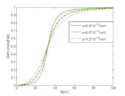
Figure 1: The Berry phase $\Gamma_{+}$ as a function of magnetic field strength $B$ with three spin-orbit coupling constants ( $\alpha=0.4\times 10^{-12}eVm$, $0.8\times 10^{-12}eVm$ and $1.2\times 10^{-12}eVm$). The other parameters used are $g=-4$, $m^{*}/m_{e}=0.05$, $g_{c}=0.01meV$, $l_{0}=80nm$, and $n=0$.

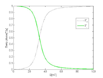
Figure 2: The Berry phases of $\Gamma_{+}$ and $\Gamma_{-}$ as a function of magnetic field strength $B$. The parameters used are $\alpha=0.4\times 10^{-12}eVm$, $g=-4$, $m^{*}/m_{e}=0.05$, $g_{c}=0.01meV$, $l_{0}=80nm$, and $n=0$.

For the illustration of the numerical results, we choose the typical parameters of the InGaAs: $g=-4$, $m^{*}/m_{e}=0.05$ ($m_{e}$ is the mass of free electron). The dot size is defined by $l_{0}=\sqrt{\hbar/m^{*}\omega_{0}}$. Figure 1 depicts the Berry phases $\Gamma_{+}$ as a function of the magnetic field strength for three spin-orbit couplings. In Figure 1, we can find that all the Berry phases change almost from 0 to $2\pi$ as the magnetic field strength varies from $20mT$ to $50mT$. When other parameters are fixed, the spin-orbit coupling constant changes as $\alpha=0.4\times 10^{-12}eVm$, $0.8\times 10^{-12}eVm$ and $1.2\times 10^{-12}eVm$, the Berry phases $\Gamma_{+}$ will have a slight movement in the figure. When $B<20mT$ and $B>50mT$, the Berry phase changes gradually, while when $20mT<B<50mT$, the Berry phase changes dramatically. As the coupling constant increases, the Berry phase changes from sharply to slowly. The Shördinger equation has two different eigenenergies when $n=0$. The two eigenenergies will give two different Berry phases. Figure 2 illustrates these two Berry phases. In Figure 2, when the others parameter are fixed, one of the Berry phase changes from 0 to $2\pi$ , while the other changes from $2\pi$ to 0 as the magnetic field strength varies from $20mT$ to $50mT$. Two Berry phases have an intersecting point at approximatively $B=33mT$, which is corresponding to the resonant point.

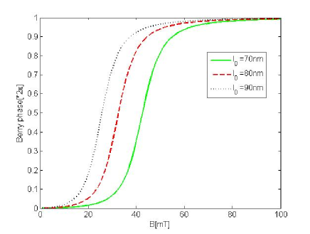
Figure 3: The Berry phases $\Gamma_{+}$ as a function of $B$ with three three different dot sizes ($l_{0}=70nm,80nm,90nm$). The parameters used are $\alpha=0.4\times 10^{-12}eVm$, $g=-4$, $m/m_{e}=0.05$, $g_{c}=0.01meV$, and $n=0$.

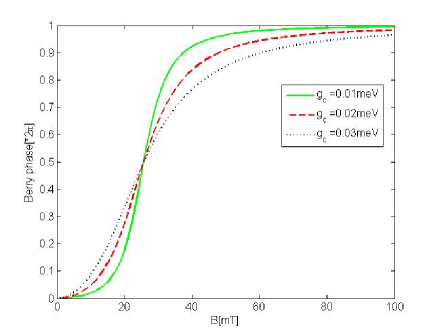
Figure 4: The Berry phases $\Gamma_{+}$ as a function of $B$ with three different light coupling constants ($g_{c}=0.01meV,0.02meV,0.03meV$). The parameters used are $\alpha=0.4\times 10^{-12}eVm$, $g=-4$, $m/m_{e}=0.05$, $l_{0}=80nm$, and $n=0$.

Figure 3 shows the effect of the dot size on the Berry phase. When dot size becomes large from 70nm to 90nm, although all three Berry phases change from 0 to $2\pi$, the threshold points of the magnetic field have a large movement. When the dot size is 70nm, the Berry phase will change dramatically at approximately 40mT, while the dot sizes are 80nm and 90nm, the turning points are approximately at 30mT and 20mT, respectively. This implies that the bigger the dot, the smaller the threshold of the magnetic field strength. Figure 4 illustrates the influence of spin-photon coupling constant on Berry phase. As the coupling constant becomes large, the Berry phase becomes less drastic as shown in Figure 4.

In a recent paper, Giuliano et al.Giuliano have designed an experimental arrangement, which is capacitively coupled the dot to one arm of a double-path electron interferometer. The phase carried by the transported electrons may be influenced by the dot. The dot’s phase gives raise to an interference term in the total conductance across the ring. More recently, Leek et al.Leek have measured Berry phase in a Ramsey fringe interference experiment. Our experimental setup proposed here is analogous with these two arrangements as shown in Figure 5. A beam light is split into two beams, one of the beams passes through the dot, and interferes with the other one. Accurate control of the light field for dot is achieved through phase and amplitude modulation of laser radiation coupled to the dot. We choose a special designed electric circuit to ensure the magnetic and laser vary synchronistically. Through detecting the interfered light, we can measure the Berry phase.

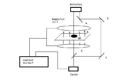
Figure 5: A sketch of a possible experimental setup to detect the Berry phase. a, b and c are three mirror, d is a beam splitter.

IV Conclusions

In conclusion, we have theoretically investigated the Berry phase in a single quantum dot in the presence of Rashba spin-orbit interaction. Berry phases as functions of magnetic field strength, dot size, spin-orbit coupling and photon-spin coupling constants are evaluated. It is shown that for a given quantum dot, the spin-orbit coupling constant and photon-spin coupling constant the Berry phase will alter dramatically from $0$ to $2\pi$ as the magnetic field strength increases. The threshold of magnetic field is dependent on the Rashba spin-orbit coupling constant, spin-photon coupling constant and the dot size. We also propose a practicable method to detect the Berry phase in such a quantum dot system. Finally, we hope that our predictions in the present work can be testified by experiments in the near future.

References

• (1) A.Shapere and F.Wilczek, Geometric Phases in Physics, (World Scientific, Singapore, 1989)
• (2) J.Anandan, Nature (London)360, 307(1992).
• (3) M.V.Berry, Proc.R.Soc.London Ser. A 392, 45(1984).
• (4) I.Fuentes-Guridi, A.Carollo, S.Bose and V.Vedral, Phys.Rev.Lett.89, 220404(2002).
• (5) X.X.Yi, L.C.Wang, and T.Y.Zheng, Phys.Rev.Lett.92, 150406(2004).
• (6) P.San-Jose, B.Scharfenberger, G.Shon, A.Shnirman, and G.Zarand, arXiv:cond-mat/0710.3931(2007).
• (7) H.Wang and K.D.Zhu, Euro.Phys.Lett82, 60006(2008).
• (8) Y.Zhang, Y.W.Tan, H.L.Stormer and P.Kim, Nature (London)438,201(2005).
• (9) M.MΓΆttΓΆnen, J.J.Vartiainen, and J.P.Pekola, Phys. Rev. Lett.100, 177201(2008).
• (10) P.J.Leek, J.M.Fink, A.Blais, Science318,1889(2007).
• (11) E.I.Rashba, Sov.Phys.Solid State2, 1109(1960)
• (12) E.B.Sonin, Phys. Rev. Lett. 99,266602(2007).
• (13) Y.A.Serebrennikov, Phys.Rev.B73,195317(2006).
• (14) J.C.Egues, G.Burkard, and D.Loss, Phys.Rev.Lett.89, 176401(2002).
• (15) E.I.Rashba, and Al.L.Efros, Phys. Rev. Lett.91, 126405 (2003).
• (16) Y.A.Bychkov and E.I.Rashba, JEPT Lett.39, 78(1984).
• (17) G.Dresselhaus Phys.Rev.B 100, 580(1955).
• (18) S.Debald and C.Emary Phys. Rev. Lett.94,226803(2005)
• (19) M.A.Marchiolli, R.J.Missori and J.A.Roversi arXiv: quant-ph/0404.008v1(2004).
• (20) D.Giuliano, P.Sodano, and A.Tagliacozzo Phys.Rev.B67, 155317(2003).