Three-Tangle for Rank-$3$ Mixed States: mixture of Greenberger-Horne-Zeilinger, W and flipped W states

Abstract

Three-tangle for the rank-three mixture composed of Greenberger-Horne-Zeilinger, W and flipped W states is analytically calculated. The optimal decompositions in the full range of parameter space are constructed by making use of the convex-roof extension. We also provide an analytical technique, which determines whether or not an arbitrary rank-$3$ state has vanishing three-tangle. This technique is developed by making use of the Bloch sphere $S^{8}$ of the qutrit system. The Coffman-Kundu-Wootters inequality is discussed by computing one-tangle and concurrences. It is shown that the one-tangle is always larger than the sum of squared concurrences and three-tangle. The physical implication of three-tangle is briefly discussed.

Entanglement is a genuine physical resource for the quantum information theoriesnielsen00 . It is at the heart of the recent much activities on the research of quantum computer. Although many new results have been derived recently for the entanglement of pure statespure , entanglement for mixed states is not much understood so far compared to the pure states. Since, however, the effect of environment generally changes the pure state into the mixed state, it is highly important to investigate the entanglement of the mixed states.

Entanglement for the bipartite mixed states, called concurrence, was studied by Hill and Wootters in Ref.form2 when the density matrix of the state has two or more zero-eigenvalue. Subsequently, Wootters extended the result of Ref.form2 to the arbitrary bipartite mixed statesform3 by making use of the time reversal operator of the spin-$1/2$ particle appropriately. In addition, the concurrence was used to derive the purely tripartite entanglement called residual entanglement or three-tangletangle1 . For three-qubit pure state $|\psi\rangle=\sum_{i,j,k=0}^{1}a_{ijk}|ijk\rangle$, the three-tangle $\tau_{3}$ becomestangle1

$$\tau_{3}=4|d_{1}-2d_{2}+4d_{3}|,$$ (1)

where

$$d_{1}=a^{2}_{000}a^{2}_{111}+a^{2}_{001}a^{2}_{110}+a^{2}_{010}a^{2}_{101}+a^{2}_{100}a^{2}_{011}$$ (2)

$$d_{2}=a_{000}a_{111}a_{011}a_{100}+a_{000}a_{111}a_{101}a_{010}+a_{000}a_{111}a_{110}a_{001}$$

$$\hskip 28.45274pt+a_{011}a_{100}a_{101}a_{010}+a_{011}a_{100}a_{110}a_{001}+a_{101}a_{010}a_{110}a_{001}$$

$$d_{3}=a_{000}a_{110}a_{101}a_{011}+a_{111}a_{001}a_{010}a_{100}.$$

The three-tangle is polynomial invariant under the local $SL(2,\mathbb{C})$ transformationver03 ; lei04 and exactly coincides with the modulus of a Cayley’s hyperdeterminantcay1845 ; miy03 . For the mixed three-qubit state $\rho$ the three-tangle is defined by making use of the convex roof constructionbenn96 ; uhlmann99-1 as

$$\tau_{3}(\rho)=\mbox{min}\sum_{i}p_{i}\tau_{3}(\rho_{i}),$$ (3)

where minimum is taken over all possible ensembles of pure states. The ensemble corresponding to the minimum of $\tau_{3}$ is called optimal decomposition.

Although the definition of three-tangle for the mixed states is simple as shown in Eq.(3), it is highly difficult to compute it. This is mainly due to the fact that the construction of the optimal decomposition for the arbitrary state is a formidable task. Even for the most simple case of rank-two state still we do not know how to construct the optimal decomposition except very rare cases.

Recently, Ref.tangle2 has shown how to construct the optimal decomposition for the rank-$2$ mixture of Greenberger-Horne-Zeilinger(GHZ) and W states:

$$\rho(p)=p|GHZ\rangle\langle GHZ|+(1-p)|W\rangle\langle W|,$$ (4)

where

$$|GHZ\rangle=\frac{1}{\sqrt{2}}\left(|000\rangle+|111\rangle\right)\hskip 28.45274pt|W\rangle=\frac{1}{\sqrt{3}}\left(|001\rangle+|010\rangle+|100\rangle\right).$$ (5)

The optimal decomposition for $\rho(p)$ was constructed with use of the fact that $\tau_{3}(|GHZ\rangle)=1$, $\tau_{3}(|W\rangle)=0$ and $\langle GHZ|W\rangle=0$. Once the optimal decompositions are constructed, it is easy to compute the three-tangle. For $\rho(p)$ the three-tangle has three-different expressions depending on the range of $p$ as following:

$$\tau_{3}(\rho(p))=\left\{\begin{array}[]{ll}0&\hskip 14.22636pt\mbox{for $0\leq p\leq p_{0}$}\\ g_{I}(p)&\hskip 14.22636pt\mbox{for $p_{0}\leq p\leq p_{1}$}\\ g_{II}(p)&\hskip 14.22636pt\mbox{for $p_{1}\leq p\leq 1$}\end{array}\right.$$ (9)

where

$$g_{I}(p)=p^{2}-\frac{8\sqrt{6}}{9}\sqrt{p(1-p)^{3}}\hskip 28.45274ptg_{II}(p)=1-(1-p)\left(\frac{3}{2}+\frac{1}{18}\sqrt{465}\right)$$ (10)

$$p_{0}=\frac{4\sqrt[3]{2}}{3+4\sqrt[3]{2}}\sim 0.6269\hskip 28.45274ptp_{1}=\frac{1}{2}+\frac{3}{310}\sqrt{465}\sim 0.7087.$$

More recently, this result was extended to the rank-$2$ mixture of generalized GHZ and generalized W states in Ref.tangle3 .

The purpose of this letter is to extend Ref.tangle2 to the case of rank-$3$ mixed states. In this paper we would like to analyze the optimal decompositions for the mixture of GHZ, W and flipped W states as

$$\rho(p,q)=p|GHZ\rangle\langle GHZ|+q|W\rangle\langle W|+(1-p-q)|\tilde{W}\rangle\langle\tilde{W}|,$$ (11)

where

$$|\tilde{W}\rangle=\frac{1}{\sqrt{3}}\left(|110\rangle+|101\rangle+|011\rangle\right).$$ (12)

For simplicity, we will define $q$ as

$$q=\frac{1-p}{n},$$ (13)

where $n$ is positive integer. Before we go further, it is worthwhile noting that $\rho(p,q)=\rho(p)$ when $n=1$ and therefore, Eq.(9) is the three-tangle in this case. When $n=\infty$, $\rho(p,q)$ can be constructed from $\rho(p)$ by local-unitary (LU) transformation $\sigma_{x}\otimes\sigma_{x}\otimes\sigma_{x}$. Since the three-tangle is LU-invariant quantity, the three-tangle of $\rho(p,q)$ with $n=\infty$ is again Eq.(9).

Now we start with three-qubit pure state

$$|Z(p,q,\varphi_{1},\varphi_{2})\rangle=\sqrt{p}|GHZ\rangle-e^{i\varphi_{1}}\sqrt{q}|W\rangle-e^{i\varphi_{2}}\sqrt{1-p-q}|\tilde{W}\rangle$$ (14)

whose three-tangle is

$$\tau_{3}(p,q,\varphi_{1},\varphi_{2})=\bigg{|}p^{2}-4p\sqrt{q(1-p-q)}e^{i(\varphi_{1}+\varphi_{2})}$$ (15)

$$-\frac{4}{3}q(1-p-q)e^{2i(\varphi_{1}+\varphi_{2})}-\frac{8\sqrt{6}}{9}\sqrt{pq^{3}}e^{3i\varphi_{1}}-\frac{8\sqrt{6}}{9}\sqrt{p(1-p-q)^{3}}e^{3i\varphi_{2}}\bigg{|}.$$

The state $|Z(p,q,\varphi_{1},\varphi_{2})\rangle$ has several interesting properties. Firstly, the mixed state $\rho(p,q)$ in Eq.(11) can be expressed in terms of $|Z(p,q,\varphi_{1},\varphi_{2})\rangle$ as following:

$$\rho(p,q)=\frac{1}{3}\Bigg{[}|Z(p,q,0,0)\rangle\langle Z(p,q,0,0)|$$ (16)

$$+|Z\left(p,q,\frac{2\pi}{3},\frac{4\pi}{3}\right)\rangle\langle Z\left(p,q,\frac{2\pi}{3},\frac{4\pi}{3}\right)|+|Z\left(p,q,\frac{4\pi}{3},\frac{2\pi}{3}\right)\rangle\langle Z\left(p,q,\frac{4\pi}{3},\frac{2\pi}{3}\right)|\Bigg{]}.$$

Secondly, $|Z(p,q,0,0)\rangle$, $|Z\left(p,q,\frac{2\pi}{3},\frac{4\pi}{3}\right)\rangle$ and $|Z\left(p,q,\frac{4\pi}{3},\frac{2\pi}{3}\right)\rangle$ have same three-tangle as shown from Eq.(15) directly. Thirdly, the numerical calculation shows that the $p$-dependence of $\tau_{3}(p,(1-p)/n,\varphi_{1},\varphi_{2})$ has many zeros depending on $\varphi_{1}$ and $\varphi_{2}$, but the largest zero $p=p_{0}$ arises when $\varphi_{1}=\varphi_{2}=0$ regardless of $n$. It can be proven rigorously with use of the implicit function theorem. The $n$-dependence of $p_{0}$ is given in Table I. Table I indicates that when $n$ increases from $n=2$, $p_{0}$ approaches to $4\sqrt[3]{2}/(3+4\sqrt[3]{2})\sim 0.6269$ from $3/4=0.75$. This is because of the fact that the three-tangle for $\rho(p,q)$ should be Eq.(9) in the $n\rightarrow\infty$ limit.

When $p\leq p_{0}$, one can construct the optimal decomposition by making use of Eq.(16) as following:

$$\rho\left(p,\frac{1-p}{n}\right)=\frac{p}{3p_{0}}\Bigg{[}|Z\left(p_{0},\frac{1-p_{0}}{n},0,0\right)\rangle\langle Z\left(p_{0},\frac{1-p_{0}}{n},0,0\right)|$$ (17)

$$\hskip 113.81102pt+|Z\left(p_{0},\frac{1-p_{0}}{n},\frac{2\pi}{3},\frac{4\pi}{3}\right)\rangle\langle Z\left(p_{0},\frac{1-p_{0}}{n},\frac{2\pi}{3},\frac{4\pi}{3}\right)|$$

$$\hskip 113.81102pt+|Z\left(p_{0},\frac{1-p_{0}}{n},\frac{4\pi}{3},\frac{2\pi}{3}\right)\rangle\langle Z\left(p_{0},\frac{1-p_{0}}{n},\frac{4\pi}{3},\frac{2\pi}{3}\right)|\Bigg{]}$$

$$\hskip 85.35826pt+\frac{p_{0}-p}{np_{0}}|W\rangle\langle W|+\frac{(n-1)(p_{0}-p)}{np_{0}}|\tilde{W}\rangle\langle\tilde{W}|.$$

Thus, we have vanishing three-tangle in this region:

$$\tau_{3}\left[\rho\left(p,\frac{1-p}{n}\right)\right]=0\hskip 28.45274pt\mbox{for $p\leq p_{0}$}.$$ (18)

Now, we consider $p_{0}\leq p\leq 1$ region. When $p=p_{0}$, Eq.(17) implies that the optimal decomposition consists of three pure states $|Z\left(p_{0},\frac{1-p_{0}}{n},0,0\right)\rangle$, $|Z\left(p_{0},\frac{1-p_{0}}{n},\frac{2\pi}{3},\frac{4\pi}{3}\right)\rangle$, and $|Z\left(p_{0},\frac{1-p_{0}}{n},\frac{4\pi}{3},\frac{2\pi}{3}\right)\rangle$ with same probability. This fact together with Eq.(16) strongly suggests that the optimal decomposition at $p_{0}\leq p$ is described by Eq.(16). As will be shown below, however, this is not true in the full range of $p_{0}\leq p\leq 1$.

The optimal decomposition (16) gives the three-tangle to $\rho(p,q)$ in a form

$$\alpha_{I}(p)=p^{2}-\frac{4\sqrt{n-1}}{n}p(1-p)-\frac{4(n-1)}{3n^{2}}(1-p)^{2}-\frac{8\sqrt{6n}\left[1+(n-1)^{3/2}\right]}{9n^{2}}\sqrt{p(1-p)^{3}}.$$ (19)

Since the three-tangle for mixed state is defined as a convex roof, $\alpha_{I}(p)$ should be convex function if it is a correct three-tangle in the range of $p_{0}\leq p\leq 1$. In order to check this we compute $d^{2}\alpha_{I}/dp^{2}$, which is

$$\frac{d^{2}\alpha_{I}(p)}{dp^{2}}=\frac{2}{9n^{2}}\left[\left\{9n^{2}+36n\sqrt{n-1}-12(n-1)\right\}-\sqrt{6n}\left\{1+(n-1)^{3/2}\right\}\frac{8p^{2}-4p-1}{\sqrt{p^{3}(1-p)}}\right].$$ (20)

Using Eq.(20) one can show that $d^{2}\alpha_{I}(p)/dp^{2}\leq 0$ when $p_{*}\leq p\leq 1$. The $n$-dependence of $p_{*}$ is given in Table I. Thus, we need to convexify $\alpha_{I}(p)$ in the region $p_{1}\leq p\leq 1$, where $p_{1}\leq p_{*}$. The constant $p_{1}$ will be determined shortly.

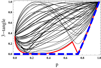
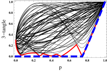
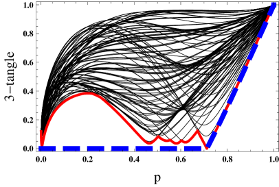
Figure 1: (color online) The plot of $p$-dependence of the Eq.(15) for various $\varphi_{1}$ and $\varphi_{2}$. We have chosen $\varphi_{1}$ and $\varphi_{2}$ from $0$ to $2\pi$ as an interval $0.3$. The three figures correspond to $n=2$ (Fig. 1a), $n=3$ (Fig. 1b) and $n=10$ (Fig. 1c) respectively. The minimum curve is plotted as a thick solid line in each figure. These figures indicate that the three-tangle in Eq.(27) (plotted as dashed line in each figure) is a convex hull of the thick solid line.

For large $p$ region one can construct the optimal decomposition as following:

$$\rho(p,q) = p|GHZ\rangle\langle GHZ|+\frac{1-p}{n}|W\rangle\langle W|+\frac{(n-1)(1-p)}{n}|\tilde{W}\rangle\langle\tilde{W}|$$

$$= p|GHZ\rangle\langle GHZ|+\frac{1-p}{1-p_{1}}\bigg{[}-p_{1}|GHZ\rangle\langle GHZ|+p_{1}|GHZ\rangle\langle GHZ|$$

$$\hskip 28.45274pt+\frac{1-p_{1}}{n}|W\rangle\langle W|+\frac{(n-1)(1-p_{1})}{n}|\tilde{W}\rangle\langle\tilde{W}|\bigg{]}$$

$$= \frac{p-p_{1}}{1-p_{1}}|GHZ\rangle\langle GHZ|+\frac{1-p}{3(1-p_{1})}\Bigg{[}|Z\left(p_{1},\frac{1-p_{1}}{n},0,0\right)\rangle\langle Z\left(p_{1},\frac{1-p_{1}}{n},0,0\right)|$$

$$\hskip 85.35826pt+|Z\left(p_{1},\frac{1-p_{1}}{n},\frac{2\pi}{3},\frac{4\pi}{3}\right)\rangle\langle Z\left(p_{1},\frac{1-p_{1}}{n},\frac{2\pi}{3},\frac{4\pi}{3}\right)|$$

$$\hskip 85.35826pt+|Z\left(p_{1},\frac{1-p_{1}}{n},\frac{4\pi}{3},\frac{2\pi}{3}\right)\rangle\langle Z\left(p_{1},\frac{1-p_{1}}{n},\frac{4\pi}{3},\frac{2\pi}{3}\right)|\Bigg{]}$$

which gives the three-tangle in a form

$$\alpha_{II}(p)=\frac{p-p_{1}}{1-p_{1}}+\frac{1-p}{1-p_{1}}\alpha_{I}(p_{1}).$$ (22)

Note that $d^{2}\alpha_{II}(p)/dp^{2}=0$. Thus, $\alpha_{II}(p)$ does not violate the convex constraint of the three-tangle in the large $p$ region. The parameter $p_{1}$ is determined by minimizing $\alpha_{II}(p)$, i.e. $\partial\alpha_{II}/\partial p_{1}=0$, which gives

$$\frac{4\sqrt{6n}\left[1+(n-1)^{3/2}\right]}{9n^{2}}\frac{2p_{1}-1}{\sqrt{p_{1}(1-p_{1})}}=1+\frac{4\sqrt{n-1}}{n}-\frac{4(n-1)}{3n^{2}}.$$ (23)

The $n$-dependence of $p_{1}$ is given in Table I. As expected $p_{1}$ is between $p_{0}$ and $p_{*}$. When $n$ increases from $n=2$, $p_{1}$ decreases from $(2+\sqrt{3})/4\sim 0.933$ to $1/2+3\sqrt{465}/310\sim 0.709$.

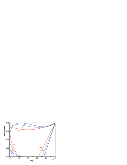
Figure 2: (color online) The $p$-dependence of one-tangle (upper solidlines), sum of squared concurrences (left solid lines) and three-tangle (right solid lines) for $n=1$, $2$ and $10$. This figure clearly indicates that not only CKW inequality (40) but also (43) hold for all integer $n$.

In summary, the three-tangle for $\rho(p,q)$ is

$$\tau_{3}(\rho(p,q))=\left\{\begin{array}[]{ll}0&\hskip 14.22636pt\mbox{for $0\leq p\leq p_{0}$}\\ \alpha_{I}(p)&\hskip 14.22636pt\mbox{for $p_{0}\leq p\leq p_{1}$}\\ \alpha_{II}(p)&\hskip 14.22636pt\mbox{for $p_{1}\leq p\leq 1$}\end{array}\right.$$ (27)

and the corresponding optimal decompositions are (17), (16), and (Three-Tangle for Rank-$3$ Mixed States: mixture of Greenberger-Horne-Zeilinger, W and flipped W states) respectively. In order to show that Eq.(27) is genuine optimal, we plotted the $p$-dependence of the three-tangles (15) for various $\varphi_{1}$ and $\varphi_{2}$ when $n=2$ (Fig. 1a), $n=3$ (Fig. 1b) and $n=10$ (Fig. 1c). These curves have been referred as the characteristic curvesoster07 . As Ref.oster07 indicated, the three-tangle is a convex hull of the minimum of the characteristic curves (thick solid lines in the figure). Fig. 1 indicates that the three-tangles (27) plotted as dashed lines are the convex characteristic curves, which implies that Eq.(27) is really optimal.

The above analysis can be applied to provide an analytical technique which decides whether or not an arbitrary rank-$3$ state has vanishing three-tangle. First we correspond our states to the qutrit states with

$$|GHZ\rangle=\left(\begin{array}[]{c}1\\ 0\\ 0\end{array}\right)\hskip 28.45274pt|W\rangle=\left(\begin{array}[]{c}0\\ 1\\ 0\end{array}\right)\hskip 28.45274pt|\tilde{W}\rangle=\left(\begin{array}[]{c}0\\ 0\\ 1\end{array}\right).$$ (37)

It is well-knownqutrit-1 that the density matrix of the arbitrary qutrit state can be represented by $\rho=(1/3)(I+\sqrt{3}\vec{n}\cdot\vec{\lambda})$, where $\vec{n}$ is $8$-dimensional unit vector and $\lambda_{i}\hskip 5.69046pt(i=1,\cdots,8)$ are Gell-Mann matrices. Thus the points on the $S^{8}$ correspond to pure qutrit states while the interior points denote the mixed states. Then, one can show straightforwardly that the pure states with vanishing three-tangle correspond to

$$|W\rangle\rightarrow\left(0,0,-\frac{\sqrt{3}}{2},0,0,0,0,\frac{1}{2}\right)$$ (38)

$$|\tilde{W}\rangle\rightarrow\left(0,0,0,0,0,0,0,-1\right)$$

$$|Z\left(p_{0},\frac{1-p_{0}}{n},0,0\right)\rangle\rightarrow\left(-\sqrt{3}\xi_{1},0,\eta_{1},-\sqrt{3}\xi_{2},0,\sqrt{3}\xi_{3},0,\eta_{2}\right)$$

$$|Z\left(p_{0},\frac{1-p_{0}}{n},\frac{2\pi}{3},\frac{4\pi}{3}\right)\rangle\rightarrow\left(\frac{\sqrt{3}}{2}\xi_{1},-\frac{3}{2}\xi_{1},\eta_{1},\frac{\sqrt{3}}{2}\xi_{2},\frac{3}{2}\xi_{2},-\frac{\sqrt{3}}{2}\xi_{3},\frac{3}{2}\xi_{3},\eta_{2}\right)$$

$$|Z\left(p_{0},\frac{1-p_{0}}{n},\frac{4\pi}{3},\frac{2\pi}{3}\right)\rangle\rightarrow\left(\frac{\sqrt{3}}{2}\xi_{1},\frac{3}{2}\xi_{1},\eta_{1},\frac{\sqrt{3}}{2}\xi_{2},-\frac{3}{2}\xi_{2},-\frac{\sqrt{3}}{2}\xi_{3},-\frac{3}{2}\xi_{3},\eta_{2}\right),$$

where $\xi_{1}=\sqrt{p_{0}(1-p_{0})/n}$, $\xi_{2}=\sqrt{n-1}\xi_{1}$, $\xi_{3}=\sqrt{n-1}(1-p_{0})/n$, $\eta_{1}=(\sqrt{3}/2)(1-(n+1)(1-p_{0})/n)$ and $\eta_{2}=(1/2)(1-3(n-1)(1-p_{0})/n)$. Thus these five points form a hyper-polyhedron in $8$-dimensional space. Then all rank-$3$ quantum states corresponding to the points in this hyper-polyhedron have vanishing three-tangle.

Now we would like to consider the Coffman-Kundu-Wootters(CKW) relationtangle1 , which is

$$4\mbox{det}\rho_{A}={\cal C}_{AB}^{2}+{\cal C}_{AC}^{2}+\tau_{3}(\psi)$$ (39)

for three-qubit pure state $|\psi\rangle$. In Eq.(39) ${\cal C}_{AB}$ and ${\cal C}_{AC}$ are the concurrences for the corresponding reduced states. Eq.(39) indicates that the entanglement of qubit $A$ is originated from both bipartite and tripartite contributions. For mixed state Ref.tangle1 has shown

$$4\min\left[\mbox{det}(\rho_{A})\right]\geq{\cal C}_{AB}^{2}+{\cal C}_{AC}^{2},$$ (40)

where minimum of one-tangle is taken over all possible decompositions of $\rho$. In Ref.tangle2 the CKW inequality (40) has been examined for the mixture of GHZ and W states. For this case it was shown that the one-tangle is always larger than the sum of squared concurrences and three-tangle.

Now, we would like to check the CKW inequality for $\rho(p,q)$ in Eq.(11) with $q=(1-p)/n$. In this case one can compute the minimum one-tangle directly, whose expression is

$$4\min\left[\mbox{det}\rho_{A}\right]=\frac{1}{9}\bigg{[}(8-4p-12q+5p^{2}+12q^{2}+12pq)$$ (41)

$$\hskip 85.35826pt+4\sqrt{pq(1-p-q)}\left(2\sqrt{6q}+2\sqrt{6(1-p-q)}-3\sqrt{p}\right)\bigg{]}.$$

Also it is straightforward to compute the sum of squared concurrences, which is

$${\cal C}_{AB}^{2}+{\cal C}_{AC}^{2}=2\left(\max\left[0,\frac{2}{3}(1-p)-\frac{1}{3}\sqrt{(3p+2q)(2+p-2q)}\right]\right)^{2}.$$ (42)

The one-tangle(upper solid lines), ${\cal C}_{AB}^{2}+{\cal C}_{AC}^{2}$(left solid lines), and three-tangle(right solid lines) are plotted in Fig. 1 for $n=1$, $n=2$ and $n=10$. This figure indicates that all quantities approach to their corresponding $n=1$ quantity when $n$ increases from $n=2$. This is consistent with the fact that $\rho(p,q)$ with $n=1$ is LU-equivalent to $\rho(p,q)$ with $n=\infty$. The inequality

$$4\min\left[\mbox{det}(\rho_{A})\right]\geq{\cal C}_{AB}^{2}+{\cal C}_{AC}^{2}+\tau_{3}$$ (43)

holds for all $n$. In the region $p_{C}\leq p\leq p_{0}$, where

$$p_{C}=\frac{(7n^{2}-4n+4)-3n\sqrt{5n^{2}-4n+4}}{(n-2)^{2}},$$ (44)

both ${\cal C}_{AB}^{2}+{\cal C}_{AC}^{2}$ and $\tau_{3}$ vanish while there is quite substantial one-tangle. Its interpretation is given in Ref.tangle2 from the mathematical point of view. However, its physical meaning is still unclear at least for us. In the region $p\geq p_{C}$ and $p\leq p_{0}$ the entanglement of the qubit $A$ mainly stems from the bipartite and tripartite correlations, respectively.

One may wonder why we do not take $q=\alpha(1-p)$ with real number $0\leq\alpha\leq 1$. For this case, however, it is unclear whether or not the $p$-dependence of $\tau_{3}(p,q,\varphi_{1},\varphi_{2})$ in Eq.(15) has maximum zero at $\varphi_{1}=\varphi_{2}=0$ regardless of $\alpha$. If this is correct, our result can be easily extended to the case of $q=\alpha(1-p)$ by changing $n\rightarrow 1/\alpha$.

There are many rank-$3$ mixed states whose three-tangles may exhibit interesting behavior. For example, let us consider the state

$$\pi(p,n)=p|GHZ,+\rangle\langle GHZ,+|+\frac{1-p}{n}|W\rangle\langle W|+\frac{(n-1)(1-p)}{n}|GHZ,-\rangle\langle GHZ,-|,$$ (45)

where $|GHZ,\pm\rangle=(1/\sqrt{2})(|000\rangle\pm|111\rangle)$. Unlike $\rho(p,n)$ discussed in the present paper $\pi(p,1)$ is not LU-equivalent with $\pi(p,\infty)$. When $n=1$, $\pi(p,1)$ is identical with $\rho(p,q)$ with $n=1$. When $n=\infty$, the three-tangle of $\pi(p,\infty)$ can be calculated by similar method and the result is $(2p-1)^{2}$. If $n$ increases from $n=2$, the three-tangle should move to $(2p-1)^{2}$ from Eq.(9) smoothly. The particular point $p=1/2$ may play a role as a fixed point. It is interesting to examine this behavior by deriving the optimal decomposition of $\pi(p,n)$ in the full range of $p$ and $n$.

Of course, it is extremely important if we develop a calculational technique, which enables us to compute the three-tangle for the arbitrary mixed states. In order to explore this issue we should develop a technique first, which enables us to compute the three-tangle for the arbitrary rank-two mixed states as Hill and Wootters did in the concurrence calculation in Ref.form2 . For the case of concurrence, however, Hill and Wootters exploited fully the magic properties of the magic basis $\{|e_{i}\rangle,i=1,\cdots,4\}$. In this basis the concurrence for the two-qubit state $|\psi\rangle$ can be expressed as $|\sum\alpha_{i}^{2}|$, where $|\psi\rangle=\sum_{i}\alpha_{i}|e_{i}\rangle$. Then this property and usual convexification technique make it possible to compute the concurrence for the arbitrary rank-two bipartite mixed states. Such a basis, however, is not found in the three-qubit system so far. Furthermore, we do not know whether or not such a basis exists in the higher-qubit system. Thus it is very difficult problem to go further this issue.

From the aspect of physics it is also of interest to investigate the physical role of the three-tangle. As shown in Ref.08-mixed the two-qubit mixed-state entanglement provides an information on the fidelity in the bipartite teleportation through noisy channels. Since the three-tangle is purely tripartite entanglement, it may give certain information in the scheme of quantum copy machine or three-party quantum teleportationkarl98 . It seems to be interesting to explore the physical role of the three-tangle in the particular real tasks.

Acknowledgement: This work was supported by the Kyungnam University Foundation Grant, 2008.

References

(1) M. A. Nielsen and I. L. Chuang, Quantum Computation and
Quantum Information (Cambridge University Press, Cambridge, England, 2000).
(2) T. C. Wei and P. M. Goldbart, Geometric measure of entanglement and
applications to bipartite and multipartite quantum states, Phys. Rev. A68 (2003)
042307 [quant-ph/0307219]; E. Jung, M. R. Hwang, H. Kim, M. S. Kim, D. K. Park, J. W. Son
and S. Tamaryan, Reduced State Uniquely Defines Groverian Measure of Original Pure
State, Phys. Rev. A77 (2008) 062317
[arXiv:0709.4292 (quant-ph)]; L. Tamaryan, DaeKil K. Park and S. Tamaryan,
Analytic Expressions for Geometric Measure of Three Qubit
States, Phys. Rev. A 77 (2008) 022325,
[arXiv:0710.0571 (quant-ph)]; L. Tamaryan, DaeKil Park, Jin-Woo Son, S. Tamaryan, Geometric
Measure of Entanglement and Shared Quantum States, Phys. Rev. A78 (2008) 032304,
[arXiv:0803.1040 (quant-ph)]; E. Jung, Mi-Ra Hwang, DaeKil Park, L. Tamaryan and S. Tamaryan,
Three-Qubit Groverian Measure, Quant. Inf. Comp. 8 (2008) 0925
[arXiv:0803.3311 (quant-ph)].
(3) S. Hill and W. K. Wootters, Entanglement of a Pair of Quantum Bits,
Phys. Rev. Lett. 78 (1997) 5022 [quant-ph/9703041].
(4) W. K. Wootters, Entanglement of Formation of an Arbitrary State
of Two Qubits, Phys. Rev. Lett. 80 (1998) 2245 [quant-ph/9709029].
(5) V. Coffman, J. Kundu and W. K. Wootters, Distributed entanglement,
Phys. Rev. A61 (2000) 052306 [quant-ph/9907047].
(6) F. Verstraete, J. Dehaene and B. D. Moor, Normal forms and entanglement
measures for multipartite quantum states, Phys. Rev. A68 (2003) 012103
[quant-ph/0105090].
(7) M. S. Leifer, N. Linden and A. Winter, Measuring polynomial invariants
of multiparty quantum states, Phys. Rev. A69 (2004) 052304 [quant-ph/0308008].
(8) A. Cayley, On the Theory of Linear Transformations, Cambridge Math.
J. 4 (1845) 193.
(9) A. Miyake, Classification of multipartite entangled states
by multidimensional determinants, Phys. Rev. A67 (2003) 012108 [quant-ph/0206111].
(10) C. H. Bennett, D. P. DiVincenzo, J. A. Smokin and W. K. Wootters,
Mixed-state entanglement and quantum error correction, Phys. Rev. A54
(1996) 3824 [quant-ph/9604024].
(11) A. Uhlmann, Fidelity and concurrence of conjugate states,
Phys. Rev. A62 (2000) 032307 [quant-ph/9909060].
(12) R. Lohmayer, A. Osterloh, J. Siewert and A. Uhlmann, Entangled
Three-Qubit States without Concurrence and Three-Tangle, Phys. Rev. Lett. 97
(2006) 260502 [quant-ph/0606071].
(13) C. Eltschka, A. Osterloh, J. Siewert and A. Uhlmann, Three-tangle
for mixtures of generalized GHZ and generalized W states, arXiv:0711.4477 (quant-ph).
(14) A. Osterloh, J. Siewert and A. Uhlmann. Tangles of superpositions and
the convex-roof extension, arXiv:0710.5909 [quant-ph].
(15) C. M. Caves and G. J. Milburn, Qutrit Entanglement,
quant-ph/9910001.
(16) E. Jung, M. R. Hwang, D. K. Park, J. W. Son and S. Tamaryan,
Mixed-state entanglement and quantum teleportation through noisy channels,
J. Phys. A: Math. Theor. 41 (2008) 385302 [arXiv:0804.4595 (quant-ph)].
(17) A. Karlsson and M. Bourennane, Quantum teleportation using
three-particle entanglement, Phys. Rev. A58 (1998) 4394.