Interplay between interference and Coulomb interaction in the ferromagnetic Anderson model with applied magnetic field

Abstract

We study the competition between interference due to multiple single-particle paths and Coulomb interaction in a simple model of an Anderson-like impurity with local-magnetic-field-induced level splitting coupled to ferromagnetic leads. The model along with its potential experimental relevance in the field of spintronics serves as a nontrivial benchmark system where various quantum transport approaches can be tested and compared. We present results for the linear conductance obtained by a spin-dependent implementation of the density matrix renormalization group scheme which are compared with a mean-field solution as well as a seemingly more advanced Hubbard-I approximation. We explain why mean-field yields nearly perfect results, while the more sophisticated Hubbard-I approach fails, even at a purely conceptual level since it breaks hermiticity of the related density matrix. Furthermore, we study finite bias transport through the impurity by the mean-field approach and recently developed higher-order density matrix equations. We find that the mean-field solution fails to describe the plausible results of the higher-order density matrix approach both quantitatively and qualitatively as it does not capture some essential features of the current-voltage characteristics such as negative differential conductance.

I Introduction

When electrons pass through a mesoscopic region, the superposition of several different single-particle transport paths can lead to interference, as, e.g., in an Aharonov-Bohm geometry with quantum dots embedded in the arms.Yacoby et al. (1995); Sigrist et al. (2004) As the size of the mesoscopic region diminishes, many-particle effects such as Coulomb blockade become increasingly important.Sohn et al. (1997) This may change the amplitudes of the competing transport paths and thereby alter the interference effect. Eventually, for sufficiently strong many-body interaction, the single-particle-paths picture breaks down and such systems should be treated using a true many-body formalism. This problem of the interplay between interference of several competing paths and many-body interaction has recently attracted a lot of attention theoretically in the general quantum-transport context Boese et al. (2001); König and Gefen (2002); Golosov and Gefen (2006); Žitko and Bonča (2006); Meden and Marquardt (2006); Tokura et al. (2007); Dinu et al. (2007); Fransson (2007); Kashcheyevs et al. (2007); Konik (2007); Lobos and Aligia (2008); Koerting et al. (2008); Weymann (2008); Lu et al. as well as from more specific points of view such as the molecular electronics, Hettler et al. (2003); Cardamone et al. (2006); Stafford et al. (2007); Begemann et al. (2008); Solomon et al. (2008); Qian et al. (2008); Ke et al. (2008) spintronics, König and Martinek (2003); Rudziński et al. (2005); Weymann and Barnas (2005); Cohen et al. (2007); Trocha and Barnaś (2007) or even full counting statisticsUrban et al. (2008) and superconducting transport.Osawa et al. (2008)

In the case of spintronics, the interference can be achieved without necessity of a multiply-connected orbital geometry due to the possibility of superposition of different purely spin amplitudes with the help of either non-collinearly magnetized leads Fransson (2005a); Weymann and Barnas (2005); Rudziński et al. (2005) or an additional spin-level splitting non-collinear with the lead magnetization. Pedersen et al. (2005); Weymann and Barnas (2005) Since experiments with strongly-interacting quantum dots and ferromagnetic contacts have recently been successfully performed van der Molen et al. (2006); Liu et al. (2007); Hauptmann et al. (2008) the spin interference effects proposed in previous workPedersen et al. (2005) and further elaborated here may be within experimental reach.

Previously, some of us considered a modelPedersen et al. (2005) consisting of a spin-$1/2$ level coupled to ferromagnetic leads with the magnetizations being either parallel or antiparallel. In addition, a magnetic field non-collinear with the spin direction of the leads was applied (see Fig. 1).

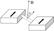
Figure 1: Sketch of our model, where the magnetic field $B$ in the central region is tilted by an angle $\phi$ with respect to the magnetization of the contacts.

For this Ferromagnetic Anderson model with an applied magnetic field $B$ (from now on nicknamed the FAB model) the linear conductance was obtained in two different regimes: without interactions on the dot, and in the cotunneling regime. For the non-interacting case with fully polarized leads, zero temperature, the bare level on resonance and a parallel lead configuration, the linear conductance can be calculated, e.g., using non-equilibrium Green functions (NEGF), and the exact result isPedersen et al. (2005) ($h$ is Planck’s constant)

$$G^{\mathrm{non-int}}=\frac{e^{2}}{h}\frac{\Gamma^{0}_{L}\Gamma^{0}_{R}}{B^{2}}\frac{\cos^{2}\phi}{1+\cos^{2}\phi\left[(\Gamma^{0}_{L}+\Gamma^{0}_{R})/2B\right]^{2}},$$ (1)

with $\Gamma^{0}_{\alpha}$ being the coupling to the leads with $\alpha=L,R$, $B$ the magnetic field times the magnetic moment of the level, and $\phi$ the angle between the magnetization in the leads and the applied magnetic field. The conductance shows anti-resonance at angles $\phi=\pi/2$ and $\phi=3\pi/2$ due to destructive interference, see Fig. 2.

Under the same conditions as stated above, the linear conductance can be obtained in the cotunneling regime ($[\Gamma_{L}^{0}+\Gamma_{R}^{0}]/B\ll 1$) even in the presence of an on-site Coulomb interaction $U$, see Eq. (5), by applying a scattering formalism: Pedersen et al. (2005)

$$G^{\mathrm{cotun}}=\frac{e^{2}\Gamma_{L}^{0}\Gamma_{R}^{0}}{h}\left[\frac{\cos^{2}(\phi/2)}{-B}+\frac{\sin^{2}(\phi/2)}{B+U}\right]^{2}.$$ (2)

In this regime, the conductance shows a cross-over from the behavior with anti-resonances at $\phi=\pi/2$ for the non-interacting case, to a spin-valve effect for $U\rightarrow\infty$ with $G^{\mathrm{cotun}}\propto\cos^{4}(\phi/2)$. That is the anti-resonances around $\phi=\pi/2$ disappear and the conductance vanishes for $\phi=\pi$ instead (see Fig. 2).

Figure 2: The linear conductance of Eq. (2), which shows the anti-resonances for non-interacting electrons (full line, $U=0$) and the spin valve behavior for strongly interacting electrons (dashed line, $U=100B$) as a function of the angle between the magnetizations of the leads and the applied magnetic field.

A simple physical picture for the situation described above is: In a basis where the Hamiltonian for the isolated dot is diagonal, the bare dot level energy is split by the magnetic field, and for non-interacting electrons the density of states has peaks at the two single-particle energies at $\mp B$, see Fig. 3. The widths of the two peaks depend on the angle $\phi$, and for fully polarized leads they are proportional to $\cos^{2}(\phi/2)$ or $\sin^{2}(\phi/2)$, respectively. For $\phi=0$ and $\phi=\pi$ one of the peaks is infinitely narrow and electrons can only pass through the other level, whereas for $\phi=\pi/2$ the peaks are equally wide resulting in the sharp anti-resonances due to interference. So the angular dependence of the conductance can be understood as interference through non-degenerate levels, which have widths depending on the angle between the magnetizations of the leads and the applied magnetic field. For a large on-site Coulomb interaction some weight of the density of states is moved away from the single-particle energies and away from the Fermi level, thereby destroying the anti-resonances.

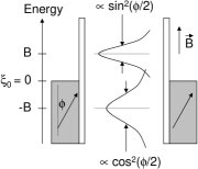
Figure 3: Schematic energy spectrum in the linear conductance regime for the non-interacting case. The bare resonant level is split due to magnetic field, and the angle between the magnetizations of the leads and the applied magnetic field is denoted by $\phi$. The widths of the two resonances depend on $\phi$ as $\cos^{2}(\phi/2)$ and $\sin^{2}(\phi/2)$, respectively.

The qualitative difference between the interacting and non-interacting regime is important, as it shows a very crucial feature in the transport through mesoscopic systems, namely that it is generally not the single-electron transport paths which determine the transport, but rather many-electron processes. Besides from leading to interesting physical effects, it also puts strong demands on the theoretical transport formalism applied to such systems, as it should be able to handle both the coherence and the interactions. It also has to be applicable for sufficiently low temperature, because otherwise thermal fluctuations will wash out the interference effect. That makes our model an excellent benchmark for transport formalisms. Including interactions, if they are sufficiently strong, is a challenge in the standard NEGF formalism where all single-particle effects including the interference are captured exactly. On the other hand, the density matrix language (generalized master equation; GME) starting from exact many-body states of the system, thus including the interaction exactly, faces problems when the broadening due to the leads comparable with level splitting (leading to interference effects) is to be incorporated. Thus, this kind of models poses significant challenges to standard transport approaches even outside notoriously difficult strongly-correlated regimes such as the Kondo regime.

Therefore, we use this model for a detailed comparison study of the performance of different transport formalisms in the potentially problematic and so far not addressed regime of broadening comparable to the level splitting $B\approx\Gamma^{0}_{\alpha}$ and arbitrarily strong interaction $U$. In particular, we test the results of higher-order, i.e. beyond mean-field, decoupling schemes based on NEGF Rudziński et al. (2005); Kashcheyevs et al. (2006); Fransson (2007) and/or many-body-states-based NEGF (Hubbard operator NEGF) approaches. Fransson et al. (2002); Sandalov et al. (2003); Fransson (2005b); Datta (2006); Frobrich and Kuntz (2006); Bergfield and Stafford ; Galperin et al. (2008) We find that the Hubbard-I approximation in the framework of NEGF,Meir et al. (1991); Fransson (2005b) frequently applied to the Anderson model with or without ferromagnetic leads,Rudziński et al. (2005); Fransson (2007); Bergfield and Stafford ; Galperin et al. (2008) gives unphysical and even mathematically wrong results for the model considered in this paper. This finding raises serious questions about the very foundation of the many-body-states-based NEGF approaches.Fransson et al. (2002); Sandalov et al. (2003); Galperin et al. (2008)

As stated above, so far only the non-interacting and the cotunneling regime have been considered (see Fig. 4), and for the latter only in linear response. In this paper, we calculate the linear conductance at zero temperature for arbitrary values of the tunneling coupling, applied magnetic field and on-site Coulomb interaction using a density matrix renormalization group (DMRG) scheme, see Sec. III. Surprisingly, in the linear response regime the results obtained using the DMRG scheme can, in certain situations, be reproduced using Green functions with a mean-field approximation, which is discussed in Sec. IV. The unexpected failure of the Hubbard-I approximation in the framework of NEGFMeir et al. (1991); Fransson (2005b) is analyzed in Sec. V. In section VI we extend the calculations beyond linear response by applying a generalized master equation formalismPedersen and Wacker (2005) which works in a basis of many-particle states and takes into account higher-order tunneling processes. In Sec. VII the failure of the mean-field Green function method for finite bias is demonstrated. Finally, we conclude on our findings in Sec. VIII. Appendix A contains the cotunneling expression for less than full polarization of the leads and off-resonant transport, and App. B presents details of the mean-field Green function calculation.

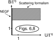
Figure 4: Sketch of the different parameter regimes. For vanishing interaction $U$, nonequilibrium Green functions provide the complete solution of the transport problem, see Eq. (1). For large level splitting, the scattering formalism allows for a quantitative description of the cotunneling events, see Eqs. (2),(29). In this work we provide results for the more intricate region of moderate level splitting and a finite on-site Coulomb interaction.

II The model system

The model Hamiltonian of the quantum dot coupled to magnetic leads is

$$H=H_{LR}+H_{T}+H_{D},$$ (3)

where

$$H_{LR}=\sum_{\alpha=L,R,k\sigma}\xi_{\alpha,k\sigma}c^{\dagger}_{\alpha,k\sigma}c_{\alpha,k\sigma}.$$ (4)

Here $\sigma=\uparrow/\downarrow$ is the spin of the electrons, $\alpha$ denotes the left or right electrodes, which are assumed to be polarized along the $z$-axis (the spin quantization axis), either parallel or anti-parallel. However, in this paper we only consider parallel magnetizations of the leads. The quantum dot is subjected to a magnetic field ${\bf B}$, which is tilted by an angle $\phi$ with respect to the $z$-axis and lies within the $xz$-plane. Note that we neglect the negative sign of the electron charge for simplicity. Thus, the energetically preferred spin direction is pointing in the direction of B throughout this paper. The dot-Hamiltonian reads ($n_{\sigma}=d^{\dagger}_{\sigma}d_{\sigma}$)

$$H_{D}=\sum_{\sigma}\xi_{0}d^{\dagger}_{\sigma}d_{\sigma}+Un_{\uparrow}n_{\downarrow}-\sum_{\sigma\sigma^{\prime}}\,\mu_{B}\mathbf{B}\cdot\boldsymbol{\tau}_{\sigma\sigma^{\prime}}d^{\dagger}_{\sigma}d_{\sigma^{\prime}},$$ (5)

where $\xi_{0}$ is the orbital quantum dot energy, $B=|\mu_{B}\mathbf{B}|$ represents the magnetic field splitting, $\boldsymbol{\tau}$ is a vector containing the Pauli spin-matrices, and $U$ is the on-site Coulomb interaction for double occupancy. In a spin basis parallel to ${\bf B}$, the dot Hamiltonian is diagonalized as

$$H_{D}=\sum_{\tilde{\sigma}}(\xi_{0}-\tilde{\sigma}B)d^{\dagger}_{\tilde{\sigma}}d_{\tilde{\sigma}}+Un_{\tilde{\uparrow}}n_{\tilde{\downarrow}},$$ (6)

where the $d_{\sigma}$ and $d_{\tilde{\sigma}}$ operators are related by the unitary rotation

$$d_{\sigma}=\sum_{\tilde{\sigma}}R_{\sigma\tilde{\sigma}}d_{\tilde{\sigma}},\quad\mathbf{R}=\left(\begin{array}[]{cc}\cos(\phi/2)&\sin(\phi/2)\\ -\sin(\phi/2)&\cos(\phi/2)\end{array}\right).$$ (7)

Finally, the tunneling Hamiltonian is

$$\begin{split}H_{T}=&\sum_{\alpha=L,R}\sum_{k\sigma}\left(t_{\alpha,k\sigma}c^{\dagger}_{\alpha,k\sigma}d_{\sigma}+\mathrm{h.c.}\right)\\ =&\sum_{\alpha=L,R}\sum_{k\sigma\tilde{\sigma}}\left(t_{\alpha,k\sigma}\mathbf{R}_{\sigma\tilde{\sigma}}c^{\dagger}_{\alpha,k\sigma}d_{\tilde{\sigma}}+\mathrm{h.c.}\right).\end{split}$$ (8)

Here we allow for the tunneling matrix element $t_{\alpha,k\sigma}$ to be spin-dependent, because the states in the leads depend on the spin direction. Note that there is no spin-flip associated with the tunneling here, i.e., there is no spin-active interface, which would require the use of a non-diagonal tunneling matrix $t_{\alpha,k\sigma\sigma^{\prime}}$. Depending on the parameters this would correspond to having an angle between the lead magnetizations, which would modify the details but not the general behavior that we discuss.

We define the energy-dependent coupling constants as

$$\Gamma_{\alpha}(\varepsilon)=2\pi\sum_{k\sigma}|t_{\alpha,k\sigma}|^{2}\delta(\varepsilon-\xi_{\alpha,k\sigma})=\sum_{\sigma}\Gamma_{\alpha,\sigma}(\varepsilon),$$ (9)

and let $P_{\alpha}$ denote the polarization of the tunneling from lead $\alpha$ defined through $\Gamma_{\alpha,\sigma}(\varepsilon)=\frac{1}{2}\left(1+\sigma P_{\alpha}\right)\Gamma_{\alpha}(\varepsilon)$. Notice that $P_{\alpha}\in[-1,1]$ such that $P_{\alpha}=\pm 1$ corresponds to full spin-$\uparrow/\downarrow$ polarization and $P_{\alpha}=0$ corresponds to unpolarized leads. For parallel (antiparallel) polarization of the leads the $P_{\alpha}$’s have the same (opposite) sign.

In the basis where the dot part of the Hamiltonian is diagonal, the coupling of the two dot states, $\tilde{\uparrow}$ and $\tilde{\downarrow}$, to the lead $\alpha$ is given by a matrix in the spin index, see also Eq. (34),

$$\Gamma_{\alpha,\tilde{\sigma}\tilde{\sigma}^{\prime}}(\varepsilon)=\frac{\Gamma_{\alpha}(\varepsilon)}{2}\times\bigg{\{}\begin{array}[]{ll}\left(1+\tilde{\sigma}P_{\alpha}\cos\phi\right)&\textrm{for }\tilde{\sigma}=\tilde{\sigma}^{\prime}\\ P_{\alpha}\sin\phi&\textrm{for }\tilde{\sigma}\neq\tilde{\sigma}^{\prime}\end{array}.$$ (10)

In the calculations using the DMRG and the density matrix technique, we use a polarization of both leads less than $1$ for technical reasons. The minority spin only introduces a smearing of the results discussed for fully polarized leads.

III Linear response: DMRG

III.1 Tight-binding Hamiltonian

In order to apply the DMRG method to the model a discretized version of the leads must be formulated. The simplest choice is to model the leads as one-dimensional semi-infinite tight-binding (TB) chains that are discretized appropriately. With this choice and denoting the hopping matrix element between the resonant level and the leads by $t_{\alpha,\sigma}$ ($\alpha=L,R$), the tight-binding Hamiltonian reads $H^{\mathrm{TB}}=\sum_{\alpha=L,R}H_{\alpha}^{\mathrm{TB}}+H_{T}^{\mathrm{TB}}+H_{D}$, where

$$H_{\alpha}^{\mathrm{TB}} = -\sum_{n=2}^{\infty}\sum_{\sigma}\frac{D}{2}\left(c^{\dagger}_{\alpha,n\sigma}c^{\phantom{{\dagger}}}_{\alpha,n-1\sigma}+c^{\dagger}_{\alpha,n-1\sigma}c^{\phantom{{\dagger}}}_{\alpha,n\sigma}\right),$$

(11)

$$H_{T}^{\mathrm{TB}} = -\sum_{\alpha=L,R}\sum_{\sigma}\left(t_{\alpha,\sigma}c^{\dagger}_{\alpha,1\sigma}d^{\phantom{{\dagger}}}_{\sigma}+\mathrm{h.c.}\right),$$ (12)

and where $H_{D}$ is given in Eq. (5). That is in the DMRG implementation we work in the lead spin-basis and do not use the diagonalized version of the dot part of the Hamiltonian. In $H_{\alpha}^{\mathrm{TB}}$, $2D$ is the bandwidth of the tight-binding chain representation of the leads corresponding to the hopping amplitude $D/2$ between the internal sites in the chains.

In order to link the different theoretical approaches applied to solve the model, an expression for the effective energy-dependent coupling constants between the single site and the tight-binding leads, $\Gamma^{\mathrm{TB}}_{\alpha,\sigma}(\varepsilon)$, must be established. For the one-dimensional tight-binding model of the leads, these are given by Datta (1995)

$$\Gamma_{\alpha,\sigma}^{\mathrm{TB}}(\varepsilon)=-2|t_{\alpha,\sigma}|^{2}~{}\mathrm{Im}\left[{g^{r}_{\alpha,\sigma}(1,1,\varepsilon)}\right],$$ (13)

where $g^{r}_{\alpha,\sigma}(1,1,\varepsilon)$ is the surface component of the retarded Green function of the semi-infinite left or right chain at energy $\varepsilon$. The surface of the tight-binding chain is the first site, and the Green function readsEconomou (1983)

$$g^{r}_{\alpha,\sigma}(1,1,z) = 2\frac{z-\sqrt{z^{2}-D^{2}}}{D^{2}},$$ (14)

where $z=\varepsilon+i\eta$ is complex, and thus the imaginary part of the Green function is finite only inside the band, $\pm D$, and is proportional to the semi-elliptic density of states. Thus the coupling constants are given by

$$\Gamma^{\mathrm{TB}}_{\alpha,\sigma}(\varepsilon)=\frac{4|t_{\alpha,\sigma}|^{2}\sqrt{D^{2}-\varepsilon^{2}}}{D^{2}}.$$ (15)

In Sec. III.2 we discuss the implementation of the polarization, and explain that half-filled leads can be used, corresponding to $\varepsilon=0$.

III.2 Modeling the polarization

Full polarization of the leads is avoided for several reasons. Most prominently, full polarization decouples one spin species in a lead completely in the sense that the hopping matrix element between the lead and the resonant level is zero for all angles. Dealing with decoupled Hilbert spaces is undesired as it creates numerical problems such as ill-conditioned matrices, making the numerical solution of the resolvent equations hard.Kühner and White (1999); Jeckelmann (2002); Bohr et al. (2006)

Furthermore, there are single points where the model itself is ill-defined for full polarization. At the angles $\phi=0$ and $\phi=\pi$ the spin-flip process of the dot is inactive because of the prefactor $\sin\phi$. Due to the full polarization also the hopping matrix element for the minority spin connecting the lead and the dot is zero. Thus the minority spin level is completely decoupled and hence has a constant occupation. The occupation of the majority spin level depends, however, on the occupation of the minority spin level through the on-site Coulomb interaction term $Un_{\uparrow}n_{\downarrow}$. That is the properties of the model for these specific angles depend on the initial occupation of the minority spin level, and no unique stationary state exists.

It should be noted that the qualitative behavior for (large) partial and full polarization are similar except for the problem for specific angles described above. It is, however, clear that a decreased polarization in the leads tends to wash out the spin dependence in the model, and in the limit of unpolarized leads all spin characteristics are lost.

There is a certain freedom of choice in the modeling of the polarization. Although the polarization is a property of the leads, it can be modeled by spin-dependent hopping matrix elements connecting the dot to the leads.Pedersen et al. (2005) There are different approaches to modeling the polarization of the leads and we have chosen the simplest one to implement in the DMRG setup. Rather than using spin-dependent filling in the leads, we use half-filled leads for both spin species, and model the polarization by modifying the hopping matrix elements connecting the leads and the dot. This is indicated in Fig. 5, where we show the DMRG setup using a momentum-space representation of the leads. This choice for the polarization simplifies the DMRG setup significantly as identical discretizations can be used for the two spin species in each lead such that the spin species are again treated equally apart from the polarization dependent hopping matrix elements,

$$t_{\alpha,\sigma} = t^{0}_{\alpha}\sqrt{\frac{1}{2}\big{(}1+\sigma P_{\alpha}\big{)}}.$$ (16)

In all calculations presented, we use identical polarizations of the two leads, $P_{L}=P_{R}=P$, such that the coupling to the leads are identical when $t^{0}_{L}=t^{0}_{R}$.

In the remainder of the article we measure all energies in units of the sum of the coupling constants at the equilibrium chemical potential, $\varepsilon=0$,

$$\Gamma^{0}=\sum_{\alpha,\sigma}\Gamma_{\alpha,\sigma}^{\mathrm{TB}}(0).$$ (17)

For the tight-binding chains this corresponds to measuring all energies in units of $\frac{4}{D}\left(|t_{L}^{0}|^{2}+|t_{R}^{0}|^{2}\right)$, see Eqs. (15),(16).

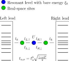
Figure 5: (Color online) Sketch of the DMRG setup for the FAB model. Notice the implementation of the polarization through the hopping matrix elements, where $t_{\alpha,\sigma}$ and the on-site Coulomb interaction $U$ are indicated in the figure. In the DMRG evaluation a single lead mapping is used in combination with a momentum-space representation of the single tight-binding lead.Bohr (2007) Here $t_{k}$ indicates a discretization dependent hopping to all states in the momentum-space.

III.3 Calculation of the conductance

In order to obtain the conductance we make use of the Meir-Wingreen formulaMeir and Wingreen (1992) rather than the Kubo formula used in previous work.Bohr et al. (2006); Bohr and Schmitteckert (2007) The evaluation of the spectral function at zero bias and for proportional couplingsHaug and Jauho (1996) can be done within a single lead framework, effectively halving the lead size. For parallel magnetizations of the leads, the FAB model falls in the linear regime within this class of models, and thus the finite size scaling for the evaluation of the spectral function is significantly better than the evaluation of the Kubo formula, enabling faster and more accurate calculations.Bohr (2007) Using DMRG we thus evaluate the two spin components of the full spectral function in separate calculations, and therefore need to recombine the spin resolved spectral functions into the total conductance,

$$G(\xi_{0},\phi)=$$ (18)

$$\frac{e^{2}}{h}\sum_{\sigma}\frac{2|t_{L,\sigma}|^{2}|t_{R,\sigma}|^{2}}{|t_{L,\sigma}|^{2}+|t_{R,\sigma}|^{2}}A_{\sigma}(\xi_{0},\phi,\omega=0),$$

where the polarization enters through the hopping matrix elements $t_{\alpha,\sigma}$, and $A_{\sigma}$ denotes the spin resolved spectral function of the dot. In this paper, we make the assumption that the hopping matrix elements between the leads and the dot are identical for both leads, $t^{0}_{L}=t^{0}_{R}$, and that the polarizations in both leads are identical, $P_{L}=P_{R}$, such that $t_{L,\sigma}=t_{R,\sigma}=t_{\sigma}$.

In order to achieve the necessary precision in the DMRG calculations a momentum-space representation of the leads is used. Although the physics takes place at the Fermi level also energies well away from the Fermi level need to be represented properly, and the discretization scheme used should support this. We use a discretization of the momentum part of each lead consisting of a logarithmic discretization that covers a large energy span, and switch to a linear discretization on the low-energy scale close to the Fermi level.Bohr and Schmitteckert (2007) All the DMRG calculations presented in this paper were performed using $55$ sites in the lead description, corresponding to $35$ sites scaled logarithmically and $20$ sites scaled linearly around the Fermi level.Bohr and Schmitteckert (2007)

It should be noted that by virtue of the DMRG method all interactions are rigorously taken into account. The approximation in the method presented lie in the use of a finite sized lead which can be benchmarked in the non-interacting limit, and as such the method used contains only controllable approximations.

III.4 Results

Using the momentum-space representation of the leads in the DMRG setup we have calculated the spectral function, and using the Meir-Wingreen formula in Eq. (18) evaluated the conductance. For different values of the magnetic field strength $B$ and the on-site Coulomb interaction strength $U$, we have calculated the conductance versus the angle $\phi$ between the magnetic field and the polarization direction. In all examples, we keep the polarization in the two leads identical, $P_{L}=P_{R}=0.8$. As evident from the Hamiltonian, the model is symmetric around $\phi=\pi$ since $\cos(2\pi-\phi)=\cos\phi$ and $\sin(2\pi-\phi)=-\sin\phi$ such that only the spin-flip term in $H_{D}$ acquires an insignificant phase [see Eq. (5)]. Therefore we confine our studies to angles in the interval $\phi\in[0,\pi]$, and the interval $\phi\in[\pi,2\pi]$ is found by reflecting the results around $\phi=\pi$.

In order to determine the discretization needed for the leads, exact diagonalization calculations for the spectral function have been performed and, using Eq. (18), compared to the NEGF results in the non-interacting limit, $U=0$ (not shown).Bohr (2007)^, By virtue of the exact diagonalization, the only error present in this approach is the error due to the finite size of the leads. The results show excellent agreement between the exact diagonalization and the Green function results for a range of parameter values, and we conclude that the modeling of the leads is sufficient for resolving the model.

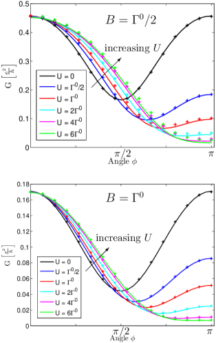
Figure 6: (Color online) The linear conductance vs. the angle $\phi$ for $B=\Gamma^{0}/2$ and $B=\Gamma^{0}$. The ‘+’ symbols are the DMRG results and the full lines are the non-equilibrium Green function results using the Hartree-Fock approximation. We apply an elliptic density of states, using Eq. (15) for the coupling constant with $D=2\Gamma^{0}$. The other parameters are $P=P_{L}=P_{R}=0.8$ and $\xi_{0}=0$. The Green function result is exact in the non-interacting limit, $U=0$, and is thus a rigorous benchmark for DMRG in this limit. The good agreement demonstrates the accuracy of the discretization, and confirms the capability of the DMRG. Furthermore there is also a surprisingly good agreement between these two methods for finite interactions as discussed in detail in Sec. IV.

Having benchmarked the DMRG setup in the known limit of $U=0$ we turn to the interesting regime of finite interactions. In Fig. 6 we show the results of the DMRG calculations (‘+’ symbols), keeping the bare level resonant, $\xi_{0}=0$. The calculations presented in each figure were performed keeping the strength of the magnetic field $B$ fixed and varying the interaction strength $U$ and the angle $\phi$, where the specific parameter values are given in the plots.

For the parameter regimes considered here the numerical zero-temperature DMRG results confirm the simple physical picture sketched in the introduction. That is the linear conductance versus the angle $\phi$ shows anti-resonances for $\phi=\pi/2$ in the non-interacting limit, and a spin-valve behavior for strong on-site interaction.

When $B/\Gamma^{0}$ decreases the maximum conductance increases as the levels move closer to resonance, but the qualitative behavior is the same when $U$ is varied. Previous work showed that for fully polarized leads and $U=0$, the anti-resonances become sharper for decreasing $B/\Gamma^{0}$ (see the left panel in Fig. 2 in Ref. Pedersen et al., 2005). Due to the finite polarization, the sharpening of the anti-resonances is not very clear in the DMRG results.

Finally we note that the cotunneling expression derived under the assumption $B\gg\Gamma^{0}$, see Eq. (29), reproduces the DMRG results fairly well already for $B=2\Gamma^{0}$ (not shown).

IV Linear response: Mean-field solution

Mean-field solutions are often problematic when considering systems with only a few degrees of freedom such as, e.g., transport through quantum dots with only a few levels contributing to the transport. In this case, the mean-field solution fails to describe Coulomb blockade Muralidharan et al. (2006) and can lead to unphysical bistabilities at finite bias due to a sudden switch between different transport modes.

Surprisingly, Fig. 6 shows that the mean-field version of the Hamiltonian from Eq. (3) actually reproduces the linear conductance results of the previous section rather well, which we will explain below.

The mean-field version of the Hamiltonian in Eq. (3) is obtained by re-writing the interaction term as consisting of a Hartree and a Fock-term

$$H_{\mathrm{Hartree}} = U(d^{\dagger}_{\tilde{\uparrow}}d_{\tilde{\uparrow}}{\langle d^{\dagger}_{\tilde{\downarrow}}d_{\tilde{\downarrow}}\rangle}+d^{\dagger}_{\tilde{\downarrow}}d_{\tilde{\downarrow}}{\langle d^{\dagger}_{\tilde{\uparrow}}d_{\tilde{\uparrow}}\rangle}),$$ (19)

$$H_{\mathrm{Fock}} = -U(d^{\dagger}_{\tilde{\uparrow}}d_{\tilde{\downarrow}}{\langle d^{\dagger}_{\tilde{\downarrow}}d_{\tilde{\uparrow}}\rangle}+d^{\dagger}_{\tilde{\downarrow}}d_{\tilde{\uparrow}}{\langle d^{\dagger}_{\tilde{\uparrow}}d_{\tilde{\downarrow}}\rangle}),$$

i.e., the replacement is $Un_{\tilde{\uparrow}}n_{\tilde{\downarrow}}\rightarrow H_{\mathrm{Hartree}}+H_{\mathrm{Fock}}$. Keeping only the Hartree-term gives a basis-dependent Hamiltonian, and for the FAB-model the two spins are correlated (for $\phi\neq 0,\pi$) due to the coupling to leads giving a non-vanishing Fock term.

From the mean-field Hamiltonian the linear conductance can be obtained using the non-equilibrium Green function formalism, and the calculation is similar to the non-interacting calculation in Ref. Pedersen et al., 2005. However here the non-interacting dot Green function is replaced with the Hartree-Fock dot Green function

$$\begin{split}\mathbf{G}&{}_{\mathrm{HF}}^{-1}(\omega)=\\ &\left(\begin{array}[]{cc}\omega-(\xi_{0}-B+U{\langle d^{\dagger}_{\tilde{\downarrow}}d_{\tilde{\downarrow}}\rangle})&+U{\langle d^{\dagger}_{\tilde{\downarrow}}d_{\tilde{\uparrow}}\rangle}\\ +U{\langle d^{\dagger}_{\tilde{\uparrow}}d_{\tilde{\downarrow}}\rangle}&\omega-(\xi_{0}+B+U{\langle d^{\dagger}_{\tilde{\uparrow}}d_{\tilde{\uparrow}}\rangle})\\ \end{array}\right).\end{split}$$ (20)

The generalized occupations have to be calculated self-consistently through the relation

$${\langle d^{\dagger}_{\tilde{\sigma}}d_{\tilde{\sigma}^{\prime}}\rangle}=\frac{-i}{2\pi}\int_{-\infty}^{\infty}d\omega~{}G^{<}_{\tilde{\sigma}^{\prime}\tilde{\sigma}}(\omega),$$ (21)

with the lesser Green function being

$$\mathbf{G}^{<}(\omega)={\rm i}f_{L}(\omega)\mathbf{G}^{r}(\omega)\mathbf{\Gamma}_{L}\mathbf{G}^{a}(\omega)+{\rm i}f_{R}(\omega)\mathbf{G}^{r}(\omega)\mathbf{\Gamma}_{R}\mathbf{G}^{a}(\omega),$$ (22)

where the expressions for the coupling constants, $\mathbf{\Gamma}_{\alpha}$, are derived in App. B.

The zero-temperature linear conductance is obtained asHaug and Jauho (1996); Datta (1995)

$$G^{\mathrm{MF}}=\frac{e^{2}}{h}\mathrm{Tr}\left[\mathbf{G}^{a}(0)\mathbf{\Gamma}_{L}\mathbf{G}^{r}(0)\mathbf{\Gamma}_{R}\right].$$ (23)

The results for $B=\Gamma^{0}/2$ and $B=\Gamma^{0}$ are shown in Fig. 6 together with the DMRG results. It is clearly seen that for $B=\Gamma^{0}$ the results agree almost exactly, but for $B<\Gamma^{0}$ deviations start to appear, especially for angles around $\pi/2$. This rather surprising success of the mean-field solutions can be understood by an inspection of the occupations, see Fig. 7:

First we notice that the couplings to the levels depend on the angle $\phi$, see Eq. (10), and consider the non-interacting case $U=0$. At $\phi=0$ the spin-$\tilde{\uparrow}$ level is roughly $80\%$ occupied due to a large broadening, but the spin-$\tilde{\downarrow}$ level is almost unoccupied due to the large $B/(\Gamma_{L,\tilde{\downarrow}\tilde{\downarrow}}+\Gamma_{R,\tilde{\downarrow}\tilde{\downarrow}})=5$. At $\phi=\pi$ the spin-$\tilde{\uparrow}$-level is almost decoupled and the occupation goes to $1$, whereas the occupation of the spin-$\tilde{\downarrow}$ level is $\sim 20\%$. For the intermediate angles, there is a smooth cross-over between the two regimes, see the black curves in Fig. 7. When calculating the occupations self-consistently for finite $U$, the overall trend does not change: $\langle n_{\tilde{\uparrow}}\rangle$ remains almost identical, and $\langle n_{\tilde{\downarrow}}\rangle$ decreases for increasing $U$, see Fig. 7.

So the reason why the mean-field solutions performs relatively well (at least at zero temperature) is that when one of the levels fluctuates the most, the other level has an occupation being either approximately zero or $1$, i.e., the products of the fluctuations vanishes. For this specific model, the success of the mean-field solution is due to the combination of the split levels and the angle dependent couplings, which means that the term $(n_{\tilde{\uparrow}}-\langle n_{\tilde{\uparrow}}\rangle)(n_{\tilde{\downarrow}}-\langle n_{\tilde{\downarrow}}\rangle)$, neglected in the mean-field Hamiltonian, remains small for all angles. The largest deviation between the mean-field results and the DMRG results is expected for the angles around $\phi=\pi/2$, which is also observed in Fig. 6.

At elevated temperatures or for even smaller magnetic fields, the mean-field solution is expected to perform worse due to larger fluctuations of the occupations, but for finite temperatures no exact results are currently available for comparison. Furthermore, while we have shown here that the mean-field solutions are somewhat fortuitously reliable to describe linear response, we demonstrate in Sec. VII that they fail for the FAB model for finite bias.

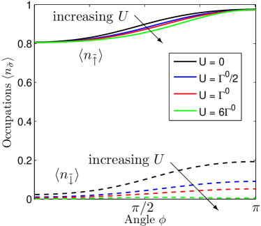
Figure 7: (Color online) The mean-field occupations vs. $\phi$ for $B=\Gamma^{0}/2$ and four different values of the on-site Coulomb interaction. The upper bunch of curves are for $\langle n_{\tilde{\uparrow}}\rangle$ and the lower ones are for $\langle n_{\tilde{\downarrow}}\rangle$. The rest of the parameters are as in Fig. 6.

V Linear response: Hubbard-I approximation

Another popular and widely used approximation is the Hubbard-I approximation (HIA) which corresponds to a decoupling of equations of motion for the Green’s functions at a higher level of the hierarchy than the simple mean-field approximation used in the previous section. Therefore, one could expect better performance of this approximation compared to the mean-field approximation. This expectation is further supported by the fact that HIA naturally arises as the lowest-order approximation in the theories developing perturbation series around the state of the isolated system, i.e. around the so-called “atomic limit”. Despite the lack of existence of the standard Wick theorem due to the non-Gaussian nature of the unperturbed system with arbitrary correlations, systematic (even renormalized) perturbation theory reportedly exists Sandalov et al. (2003); Ovchinnikov and Val’kov (2004) and HIA is in a certain sense the lowest order in that expansion. Indeed, it turns out that HIA can rather simply and yet correctly describe the non-trivial effects of single-level broadening in the Coulomb blockade regime of transport studied by other sophisticated methodsPedersen and Wacker (2005); Könemann et al. (2006) and confirmed experimentally.Könemann et al. (2006) Therefore HIA appears to be the solution to the problem of a simultaneous description of interference/broadening and interaction.

However, this optimistic picture breaks down as soon as more complicated systems are addressed, namely, any system where coherence between different transport channels is involved. The FAB model is one such example and we will demonstrate the breakdown of HIA for this model. A similar situation arises for the problem of a single spin-degenerate level with local Coulomb interaction coupled to superconducting leads in the so-called $\pi$-junction regime, where the Josephson supercurrent is observed. The HIA is known to fail to predict this theoretically and experimentally well-established fact, see e.g. Ref. Osawa et al., 2008, Fig. 4a. The situation in the case of the FAB model is even more severe since the HIA failure is not just physical, as in the superconducting case, but the results are even mathematically inconsistent. Fundamental analytical identities such as $\left(\mathbf{G}^{r}\right)^{\dagger}=\mathbf{G}^{a}$ and, consequently, the hermiticity of the density matrix is broken within the HIA.

To demonstrate this explicitly, we use the Hamiltonian in Eq. (3) and perform analogous derivations as in Refs. Rudziński et al., 2005, Fransson, 2005b for simpler models without any magnetization at all or without the local splitting, respectively. We arrive at the matrix equation

$$\mathbf{G}(\varepsilon)=\mathbf{g}(\varepsilon)+\mathbf{g}(\varepsilon)\mathbf{\Sigma}(\varepsilon)\mathbf{G}(\varepsilon)$$ (24)

for the causal Green function $G_{\tilde{\sigma}\tilde{\sigma}^{\prime}}(\varepsilon)$ (in energy representation) of the central dot. Here

$$\Sigma_{\tilde{\sigma}\tilde{\sigma}^{\prime}}(\varepsilon)=\sum_{\alpha k\sigma}|t_{\alpha,k\sigma}|^{2}\left(\mathbf{R}^{\dagger}\right)_{\tilde{\sigma}\sigma}\frac{1}{\varepsilon-\xi_{\alpha,k\sigma}}\mathbf{R}_{\sigma\tilde{\sigma}^{\prime}}.$$ (25)

is the self-energy matrix due to the coupling to the contacts, and we introduced the auxiliary Green function

$$\mathbf{g}(\varepsilon)=\left(\begin{array}[]{cc}\frac{\varepsilon-\xi_{{\tilde{\uparrow}}}-U(1-\langle d^{\dagger}_{{\tilde{\downarrow}}}d_{{\tilde{\downarrow}}}\rangle)}{(\varepsilon-\xi_{{\tilde{\uparrow}}})(\varepsilon-\xi_{{\tilde{\uparrow}}}-U)}&\frac{-U\langle d^{\dagger}_{{\tilde{\downarrow}}}d_{{\tilde{\uparrow}}}\rangle}{(\varepsilon-\xi_{{\tilde{\uparrow}}})(\varepsilon-\xi_{{\tilde{\uparrow}}}-U)}\\ \frac{-U\langle d^{\dagger}_{{\tilde{\uparrow}}}d_{{\tilde{\downarrow}}}\rangle}{(\varepsilon-\xi_{{\tilde{\downarrow}}})(\varepsilon-\xi_{{\tilde{\downarrow}}}-U)}&\frac{\varepsilon-\xi_{{\tilde{\downarrow}}}-U(1-\langle d^{\dagger}_{{\tilde{\uparrow}}}d_{{\tilde{\uparrow}}}\rangle)}{(\varepsilon-\xi_{{\tilde{\downarrow}}})(\varepsilon-\xi_{{\tilde{\downarrow}}}-U)}\end{array}\right)\mathbf{,}$$ (26)

where $\xi_{{\tilde{\uparrow}}/{\tilde{\downarrow}}}=\xi_{0}\mp B$ are the level energies in the basis parallel to ${\bf B}$ as given in Eq. (6). For vanishing splitting, $B=0$, these are precisely the Eqs. (15)–(21) of Ref. Rudziński et al., 2005. The retarded and advanced Green function are then again obtained by ${\bf G}^{r/a}(\varepsilon)={\bf G}(\varepsilon\pm{\rm i}0^{+})$, respectively. In addition, we define the retarded and advanced components of the other functions in the same way.

A general condition relating the retarded and advanced Green’s functions is $\left(\mathbf{G}^{r}\right)^{\dagger}=\mathbf{G}^{a}$. As Eq. (24) implies

$$\mathbf{g}^{r/a}=\left[\left(\mathbf{G}^{r/a}\right)^{-1}+\mathbf{\Sigma}^{r/a}\right]^{-1},$$ (27)

and $\left(\mathbf{\Sigma}^{r}\right)^{\dagger}=\mathbf{\Sigma}^{a}$ from Eq. (25) this requires $\left(\mathbf{g}^{r}\right)^{\dagger}=\mathbf{g}^{a}$. This is, however, only compatible with Eq. (26) if the off-diagonal elements are mutually complex conjugated. For non-zero coherences $\langle d^{\dagger}_{{\tilde{\downarrow}}}d_{{\tilde{\uparrow}}}\rangle=\langle d^{\dagger}_{{\tilde{\uparrow}}}d_{{\tilde{\downarrow}}}\rangle^{*}\neq 0$ and finite level splitting $\xi_{{\tilde{\uparrow}}}\neq\xi_{{\tilde{\downarrow}}}$ pertinent to the FAB model this condition is not satisfied and, thus, HIA breaks the necessary mathematical condition for the Green’s functions. Similarly, self-consistent evaluation of the (generalized) populations in the spirit of Eq. (21) in thermal equilibrium (since we study currently the linear response only) would yield a non-hermitian density matrix, yet another mathematical problem stemming from the inconsistency of the HIA equations.

It should be stressed that the inconsistency only shows up if both the local level splitting and the coherences between different spin states (stemming from non-collinear magnetization arrangement) are present. Therefore, the inconsistency has apparently not been noticed beforeRudziński et al. (2005); Fransson (2005b) since previously employed models do not contain both necessary ingredients.

Nevertheless, the FAB model is both mathematically and physically a realistic model and the failure of HIA reveals problems inherent in that approximation. As mentioned before, the HIA is in some sense the lowest-order expansion in reportedly systematic theories based on Hubbard operator Green’s functions.Sandalov et al. (2003) One can show that the same problems carry over to the many-body formalism, see Ref. Fransson, 2005b for a pedagogical overview of the connection between the formulation of HIA in the standard as well as the many-body formalism.

VI Finite bias: 2vN approach

So far we have only considered linear response and zero temperature. In this section we apply a density matrix formalism developed in Ref. Pedersen and Wacker, 2005, giving access to the regime of finite bias and finite temperature. The method works in a basis of many-particle eigenstates for the dot Hamiltonian, thereby including all interactions on the dot exactly. Correlated transitions between the lead and the dot states with up to two different electron states are included exactly, which suggest the notation second order von Neumann approach (2vN). By solving the resulting set of equations for the steady-state, a certain class of higher-order processes are also included. Interference effects are also included by a full treatment of the nondiagonal density matrix elements.

The dot part of the Hamiltonian, $H_{D}$, has four many-particle eigenstates $\{|0\rangle,|\tilde{\uparrow}\rangle,|\tilde{\downarrow}\rangle,|2\rangle\}$, where $|2\rangle=\tilde{d}^{\dagger}_{\downarrow}\tilde{d}^{\dagger}_{\uparrow}|0\rangle$, and the energies are $0,E_{\tilde{\uparrow}}=\xi_{0}-B,E_{\tilde{\downarrow}}=\xi_{0}+B$ and $E_{2}=E_{\tilde{\uparrow}}+E_{\tilde{\downarrow}}+U$, respectively. Inserting a complete set of dot states in the tunneling Hamiltonian from Eq. (8) gives

$$\begin{split}H_{T}=\sum_{k\sigma\alpha,ab}\left(T_{ba}(k\sigma\alpha)|b\rangle\langle a|c_{\alpha,k\sigma}+c^{{\dagger}}_{\alpha,k\sigma}|a\rangle\langle b|T_{ba}^{*}(k\sigma\alpha)\right)\end{split}$$ (28)

where $a,b$ denotes the dot many-particle eigenstates and $T_{ba}(k\sigma\alpha)=\sum_{\mu}t_{\alpha,k\sigma}^{*}R_{\sigma\mu}\langle b|d_{\mu}^{\dagger}|a\rangle$ are the couplings between these states and the lead states.

Inserting these coupling matrix elements and eigenenergies in Eqs. (10),(11) in Ref. Pedersen and Wacker, 2005 gives a closed set of equations for the elements of the reduced density matrix, which can be solved numerically. As for the DMRG calculation we assume the leads to be $80\%$ polarized. Significantly larger polarizations ($\approx 1$) are difficult to handle numerically, especially in the linear conductance regime. This also limits the values for the bias voltages and temperatures which can be used.

For the finite bias calculations presented here, we use a constant density of states, so that effects due to the change of the chemical potentials are not superimposed by changes in the contact couplings. For numerical purposes, we implement a finite band width with elliptically shaped edges at $0.95D<|\varepsilon|<D$, where $D$ surpasses all other relevant energy scales. In all plots, the bias voltage $V$ is applied symmetrically, $\mu_{L}=-\mu_{R}=eV/2$.

Before considering finite bias, we have carefully inspected the results for low bias ($eV/\Gamma^{0}=0.05-0.1$) and low temperature ($k_{B}T/\Gamma^{0}=0.05-0.1$) for $B/\Gamma^{0}=0.5,1,2$ for all angles $\phi$ (not shown). For the non-interacting case, the exact NEGF results are reproduced for all parameters tested. From the low-bias results we have extracted a numerical value for the linear conductance, and the results show almost quantitative agreement with the exact DMRG results for all tested values of $U$ and all angles. The discrepancies can be attributed to the (small but) finite bias and the finite temperature used in the density matrix calculation. We conclude that the 2vN approach is capable of describing the effect of the interactions and the coherence in the low-bias regime for the model system considered.

Fig. 8a) shows the current versus bias voltage for different angles, where the bare level is on resonance, $\xi_{0}=0$, $B=2\Gamma^{0}$ and an on-site Coulomb interaction $U=8\Gamma^{0}$. Shoulders in the current are expected if half the bias matches the single-electron transition energies in the dot. This happens at $eV/\Gamma^{0}=4$ for the transitions ${|0\rangle}\rightarrow{|\tilde{\uparrow}\rangle}$ and ${|0\rangle}\rightarrow{|\tilde{\downarrow}\rangle}$, at $eV/\Gamma^{0}=12$ for ${|\tilde{\downarrow}\rangle}\rightarrow{|2\rangle}$, and finally at $eV/\Gamma^{0}=20$ for ${|\tilde{\uparrow}\rangle}\rightarrow{|2\rangle}$.

In the low-bias regime, $eV/\Gamma^{0}<4$, the current is suppressed when the angle $\phi$ is increased from $0$ to $\pi$ due to the spin-valve effect (see also, e.g., Fig. 6 for large $U/\Gamma^{0}$).

In the intermediate regime $12<eV/\Gamma^{0}<20$, the current shows a very pronounced angular dependence, with a significant current drop between $\phi=0$ and $\phi=\pi$. For $\phi\approx\pi$ one even detects negative differential conductance around $eV=12\Gamma^{0}$. In this region, the lower spin level $\tilde{\uparrow}$ can be filled not only by the process ${|0\rangle}\rightarrow{|\tilde{\uparrow}\rangle}$ but also by ${|\tilde{\downarrow}\rangle}\rightarrow{|2\rangle}$. It is thus more likely to be filled compared to lower biases $eV<12\Gamma^{0}$. In the case $\phi=0$, $\tilde{\uparrow}$ is aligned with the lead polarization and therefore exhibits high tunneling rates. Thus its increased occupation probability goes along with an increase of current around $eV=12\Gamma^{0}$. In contrast, for $\phi=\pi$, $\tilde{\uparrow}$ is pointing against the lead polarization and therefore has a low tunneling rate, explaining the drop of current around $eV=12\Gamma^{0}$. For intermediate angles there is a smooth cross-over between the two limits. Here the non-diagonal elements of the density matrix are non-vanishing and quantum coherence plays a role, as the two dot states are superpositions of the lead spins. Off-diagonal elements are also important to include in transport through dots coupled to non-collinear ferromagnetic leads, even in the absence of an applied magnetic field.Braun et al. (2004)^,

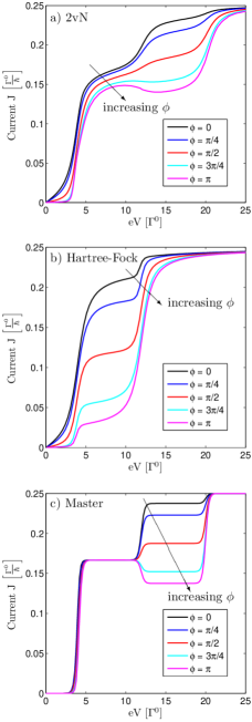
Figure 8: (Color online) The current versus bias voltage for five different angles $\phi$ obtained using the 2vN density matrix formalism (a), the mean-field Hartree-Fock approach (b), and the master equation approach (c). The parameters are: $\xi_{0}=0$, $B=2\Gamma^{0}$, $U=8\Gamma^{0}$, $k_{B}T=0.1\Gamma^{0}$, $P_{L}=P_{R}=0.8$ and the bias is applied symmetrically. For the 2vN-method we used a constant density of states with a half band-width $D=20\Gamma^{0}$, see the main text, while for the Hartree-Fock calculation the wide-band limit is applied, i.e. the real-part of the self-energy was neglected.

VII Finite bias: mean-field NEGF and master equation

Figure 8b) shows the current versus applied bias calculated using the Hartree-Fock mean-field version of the Hamiltonian, see Eqs. (19)-(22) and App. B, within the NEGF formalism using a self-consistent calculation of the occupations, see, e.g., Ref. Datta, 1995. The parameters are identical to Fig. 8a) in order to allow for a direct comparison.

In the low-bias regime ($eV<4\Gamma^{0}$), where the average occupations $\langle n_{\tilde{\uparrow}}\rangle$, $\langle n_{\tilde{\downarrow}}\rangle$ are close to one and zero, respectively, the results agree with the 2vN formalism of Sec. VI. This goes well with the observation from section IV, that the conductance is well reproduced within the mean-field model.

In the region $4<eV/\Gamma^{0}<12$, we find $\langle n_{\tilde{\uparrow}}\rangle\approx 0.5$ as the lower energy state $\tilde{\uparrow}$ is in the window between the Fermi levels with symmetric coupling to both contacts. Thus the higher energy state $\tilde{\downarrow}$ has the energy $B+U/2=6\Gamma^{0}$ which is above the emitter Fermi level and $\langle n_{\tilde{\downarrow}}\rangle\approx 0$. If $\tilde{\uparrow}$ is aligned with the lead polarization (i.e. $\phi=0$), the current is larger, while it is low for $\phi=\pi$ as seen in Fig. 8b). Finally, at $eV/\Gamma^{0}>12$, the upper level $\tilde{\downarrow}$ enters the window between the Fermi levels, takes an average occupation $\langle n_{\tilde{\downarrow}}\rangle\approx 0.5$, and contributes also to the current. The repulsion of the levels by $U/2$ is an artefact of the mean-field model, and correspondingly neither the current values nor the shoulders agree with the more detailed 2vN results shown in Fig. 8a).

Fig. 8c) shows the corresponding result from the master equation approach Kinaret et al. (1992); Pfannkuche and Ulloa (1995); Muralidharan et al. (2006) where the occupations of the many-particle states are determined by electron hopping processes to and from the leads. While this approach does not provide any current for low biases, where cotunneling dominates the transport, it provides reliable results for the current plateaus. In particular, the occurrence of negative differential conductance for $\phi\approx\pi$ for biases around $12\Gamma^{0}/e$ is confirmed. Note that the presence of pronounced steps of width $k_{B}T$ is due to the entire neglect of broadening in this approach. Similar results are obtained by taking into account nondiagonal density matrices within the 1vN approach Pedersen et al. (2007) (not shown).

VIII Conclusion

In this article, we provided a full description of the Ferromagnetic Anderson model with applied magnetic field $B$ (FAB). We have successfully implemented the density matrix renormalization group (DMRG) method, which provides the linear conductance for arbitrary strength of the on-site Coulomb interaction and arbitrary level splitting. The data interpolate between the known results of non-equilibrium Green functions (NEGF) for zero interaction and the cotunneling results for large level splitting. A key result is the strong suppression of conductance with increasing on-site Coulomb interaction if the magnetic field on the dot is opposite to the lead polarization.

The DMRG results can serve as a benchmark for different approaches, where we find that both the second order von Neumann (2vN) approach and the NEGF approach with mean-field interaction give reliable results for the conductance. While the 2vN approach also provides plausible results for finite bias, the mean-field NEGF fails due to the wrong treatment of partially occupied states.

For finite bias the 2vN approach predicts a strong dependence of the current on the direction of the magnetic field in the intermediate bias region. Here negative differential conductance is predicted if the magnetic field on the dot is opposite to the lead polarization. This feature can also be qualitatively obtained from the simpler master equation approach.

Finally we have shown that the Hubbard I approximation leads to unphysical results for this particular model. This shows that the FAB model constitutes a sensitive test case for different approaches due to its involved interplay between interference, broadening, and interaction.

Appendix A Cotunneling expression

The expression for the cotunneling current in Eq. (2) can easily be generalized to arbitrary polarization and off-resonant transport, $\xi_{0}\neq 0$. For identical polarizations of the leads, $P_{L}=P_{R}=P$, it reads

$$\begin{split}G^{\mathrm{cotun}}=&\frac{e^{2}\Gamma_{L}^{0}\Gamma_{L}^{0}}{2\pi\hbar}\Bigg{[}\left(\frac{1+P}{2}\right)^{2}\left(\frac{\cos^{2}(\phi/2)}{\xi_{0}-B}+\frac{\sin^{2}(\phi/2)}{\xi_{0}+B+U}\right)^{2}\\ &+2\frac{(1+P)(1-P)}{4}\left(\frac{-\sin(\phi/2)\cos(\phi/2)}{\xi_{0}-B}+\frac{\sin(\phi/2)\cos(\phi/2)}{\xi_{0}+B+U}\right)^{2}+\left(\frac{1-P}{2}\right)^{2}\left(\frac{\sin^{2}(\phi/2)}{\xi_{0}-B}+\frac{\cos^{2}(\phi/2)}{\xi_{0}+B+U}\right)^{2}\Bigg{]}.\end{split}$$ (29)

Appendix B Equations for the NEGF solution

For completeness we present here the equations for the non-equilibrium Green function calculations within the Hartree-Fock approximation. Using the equation-of-motion technique, the Green functions in the diagonal basis arePedersen et al. (2005)

$$\mathbf{G}^{r,a}(\varepsilon) =\left(\mathbf{G}_{\mathrm{HF}}^{-1}-\mathbf{\Sigma}^{r,a}_{L}(\varepsilon)-\mathbf{\Sigma}^{r,a}_{R}(\varepsilon)\right)^{-1},$$ (30a)

$$[\mathbf{\Sigma}^{r,a}_{\alpha}(\varepsilon)]_{\tilde{\sigma}\tilde{\sigma}^{\prime}} =\sum_{k\sigma}(\mathbf{R}^{\dagger})_{\tilde{\sigma}\sigma}|t_{\alpha,k\sigma}|^{2}g^{r,a}_{\alpha,k\sigma}(\varepsilon)\mathbf{R}_{\sigma\tilde{\sigma}^{\prime}}\,,$$ (30b)

where $g^{r,a}_{\alpha,k\sigma}(\varepsilon)=(\varepsilon-\xi_{\alpha,k\sigma}\pm i0^{+})^{-1}$ and $\mathbf{\Gamma}_{\alpha}=-i\left[\mathbf{\Sigma}^{r}_{\alpha}-\mathbf{\Sigma}^{a}_{\alpha}\right]$. The Green function $\mathbf{G}_{\mathrm{HF}}^{-1}(\varepsilon)$ is stated in Eq. (20).

For the tight-binding chain of Sec. III with elliptic bands we find

$$\begin{split}\Gamma_{\alpha}(\varepsilon)\equiv&2\pi\sum_{k\sigma}|t_{\alpha,k\sigma}|^{2}\delta(\varepsilon-\xi_{\alpha,k\sigma})\\ =&\sum_{\sigma}\Gamma^{\mathrm{TB}}_{\alpha,\sigma}(\varepsilon)=\frac{4|t_{\alpha}^{0}|^{2}\sqrt{D^{2}-\varepsilon^{2}}}{D^{2}}\,,\end{split}$$ (31)

where Eqs. (15), (16) have been used. The ${\tilde{\uparrow}}{\tilde{\uparrow}}$-component of the self-energy becomes

$$\begin{split}\left[\Sigma^{r,a}_{\alpha}(\varepsilon)\right]_{{\tilde{\uparrow}}{\tilde{\uparrow}}}=&\sum_{k\sigma}\frac{(\mathbf{R}^{\dagger})_{{\tilde{\uparrow}}\sigma}|t_{\alpha,k\sigma}|^{2}\mathbf{R}_{\sigma{\tilde{\uparrow}}}}{\varepsilon-\xi_{\alpha,k\sigma}\pm i0^{+}}\\ =&\frac{1}{2}(1+P_{\alpha}\cos\phi)\int\frac{d\varepsilon^{\prime}}{2\pi}\frac{\Gamma_{\alpha}(\varepsilon^{\prime})}{\varepsilon-\varepsilon^{\prime}\pm i0^{+}}\,,\end{split}$$ (32)

where we used the definition of the polarization [see below Eq. (9)].

The principal part of the integral can be found analytically for the elliptic density of states

$$\mathcal{P}\int^{D}_{-D}\frac{d\varepsilon^{\prime}}{2\pi}\frac{\Gamma_{\alpha}(\varepsilon^{\prime})}{\varepsilon-\varepsilon^{\prime}}=\frac{\Gamma_{\alpha}(0)\varepsilon}{2D}~{}~{}\mathrm{for}~{}|\varepsilon|<D,$$ (33)

where it has been used that $\Gamma_{\alpha}(0)=4|t^{0}_{\alpha}|^{2}/D$.

The other components are calculated similarly, and the full expression for the self-energy becomes

$$\Sigma^{r,a}_{\alpha}(\varepsilon)=\frac{1}{2}\left(\begin{array}[]{cc}1+P_{\alpha}\cos\phi&P_{\alpha}\sin\phi\\ P_{\alpha}\sin\phi&1-P_{\alpha}\cos\phi\\ \end{array}\right)\\ \times\left[\frac{\varepsilon\Gamma_{\alpha}(0)}{2D}\mp\frac{i\Gamma_{\alpha}(\varepsilon)}{2}\right].$$ (34)

After a self-consistent evaluation of the Green functions, the current can within the mean-field approximation be evaluated as

$$\begin{split}J^{\mathrm{MF}}=\frac{1}{2\pi\hbar}\int_{-\infty}^{\infty}d\varepsilon\mathrm{Tr}&\left[\mathbf{G}^{a}(\varepsilon)\mathbf{\Gamma}_{L}(\varepsilon)\mathbf{G}^{r}(\varepsilon)\mathbf{\Gamma}_{R}(\varepsilon)\right]\\ &~{}\times\left[f_{L}(\varepsilon)-f_{R}(\varepsilon)\right],\end{split}$$ (35)

with $f_{\alpha}(\varepsilon)=1/\left[e^{(\varepsilon-\mu_{\alpha})/k_{B}T}+1\right]$, $\alpha=L,R$, being the Fermi function.

References

- Yacoby et al. (1995) A. Yacoby, M. Heiblum, D. Mahalu, and H. Shtrikman, Phys. Rev. Lett. 74, 4047 (1995).
- Sigrist et al. (2004) M. Sigrist, A. Fuhrer, T. Ihn, K. Ensslin, S. E. Ulloa, W. Wegscheider, and M. Bichler, Phys. Rev. Lett. 93, 066802 (2004).
- Sohn et al. (1997) L. L. Sohn, L. P. Kouwenhoven, and G. Schön, eds., Mesoscopic Electron Transport, vol. E 345 of NATO ASI Series (Kluwer Academic Publishers, Boston, 1997).
- Boese et al. (2001) D. Boese, W. Hofstetter, and H. Schoeller, Phys. Rev. B 64, 125309 (2001).
- König and Gefen (2002) J. König and Y. Gefen, Phys. Rev. B 65, 045316 (2002).
- Golosov and Gefen (2006) D. I. Golosov and Y. Gefen, Phys. Rev. B 74, 205316 (2006).
- Žitko and Bonča (2006) R. Žitko and J. Bonča, Phys. Rev. B 74, 045312 (2006).
- Meden and Marquardt (2006) V. Meden and F. Marquardt, Phys. Rev. Lett. 96, 146801 (2006).
- Tokura et al. (2007) Y. Tokura, H. Nakano, and T. Kubo, New J. Phys. 9, 113 (2007).
- Dinu et al. (2007) I. V. Dinu, M. Ţolea, and A. Aldea, Phys. Rev. B 76, 113302 (2007).
- Fransson (2007) J. Fransson, Phys. Rev. B 76, 045416 (2007).
- Kashcheyevs et al. (2007) V. Kashcheyevs, A. Schiller, A. Aharony, and O. Entin-Wohlman, Phys. Rev. B 75, 115313 (2007).
- Konik (2007) R. M. Konik, Phys. Rev. Lett. 99, 076602 (2007).
- Lobos and Aligia (2008) A. M. Lobos and A. A. Aligia, Phys. Rev. Lett. 100, 016803 (2008).
- Koerting et al. (2008) V. Koerting, J. Paaske, and P. Wölfle, Phys. Rev. B 77, 165122 (2008).
- Weymann (2008) I. Weymann, Phys. Rev. B 78, 045310 (2008).
- (17) H. Lu, Z. Chen, R. Lü, and B. Zhu, arXiv:0806.2511.
- Hettler et al. (2003) M. H. Hettler, W. Wenzel, M. R. Wegewijs, and H. Schoeller, Phys. Rev. Lett. 90, 076805 (2003).
- Cardamone et al. (2006) D. Cardamone, C. Stafford, and S. Mazumdar, Nano Letters 6, 2422 (2006).
- Stafford et al. (2007) C. A. Stafford, D. M. Cardamone, and S. Mazumdar, Nanotechnology 18, 424014 (2007).
- Begemann et al. (2008) G. Begemann, D. Darau, A. Donarini, and M. Grifoni, Phys. Rev. B 77, 201406 (2008).
- Solomon et al. (2008) G. C. Solomon, D. Q. Andrews, T. Hansen, R. H. Goldsmith, M. R. Wasielewski, R. P. V. Duyne, and M. A. Ratner, J. Chem. Phys. 129, 054701 (2008).
- Qian et al. (2008) Z. Qian, R. Li, X. Zhao, S. Hou, and S. Sanvito, Phys. Rev. B 78, 113301 (2008).
- Ke et al. (2008) S.-H. Ke, W. Yang, and H. U. Baranger (2008), arXiv:0806.3593.
- König and Martinek (2003) J. König and J. Martinek, Phys. Rev. Lett. 90, 166602 (2003).
- Rudziński et al. (2005) W. Rudziński, J. Barnaś, R. Świrkowicz, and M. Wilczyński, Phys. Rev. B 71, 205307 (2005).
- Weymann and Barnas (2005) I. Weymann and J. Barnas, Eur. Phys. J. B 46, 289 (2005).
- Cohen et al. (2007) G. Cohen, O. Hod, and E. Rabani, Phys. Rev. B 76, 235120 (2007).
- Trocha and Barnaś (2007) P. Trocha and J. Barnaś, Phys. Rev. B 76, 165432 (2007).
- Urban et al. (2008) D. Urban, J. König, and R. Fazio, Phys. Rev. B 78, 075318 (2008).
- Osawa et al. (2008) K. Osawa, N. Yokoshi, and S. Kurihara (2008), arXiv:0806.0527.
- Fransson (2005a) J. Fransson, Europhys. Lett. 70, 796 (2005a).
- Pedersen et al. (2005) J. N. Pedersen, J. Q. Thomassen, and K. Flensberg, Phys. Rev. B 72, 045341 (2005).
- van der Molen et al. (2006) S. J. van der Molen, N. Tombros, and B. J. van Wees, Phys. Rev. B 73, 220406 (2006).
- Liu et al. (2007) R. S. Liu, D. Suyatin, H. Pettersson, and L. Samuelson, Nanotechnology 18, 055302 (2007).
- Hauptmann et al. (2008) J. Hauptmann, J. Paaske, and P. Lindelof, Nature Physics 4, 373 (2008).
- Kashcheyevs et al. (2006) V. Kashcheyevs, A. Aharony, and O. Entin-Wohlman, Phys. Rev. B 73, 125338 (2006).
- Fransson et al. (2002) J. Fransson, O. Eriksson, and I. Sandalov, Phys. Rev. Lett. 88, 226601 (2002).
- Sandalov et al. (2003) I. Sandalov, B. Johansson, and O. Eriksson, Int. J Quantum Chem. 94, 113 (2003).
- Fransson (2005b) J. Fransson, Phys. Rev. B 72, 075314 (2005b).
- Datta (2006) S. Datta (2006), arXiv:cond-mat/0603034v1.
- Frobrich and Kuntz (2006) P. Frobrich and P. Kuntz, Physics Reports 432, 223 (2006).
- (43) J. P. Bergfield and C. A. Stafford, arXiv:0803.2756.
- Galperin et al. (2008) M. Galperin, A. Nitzan, and M. A. Ratner, Phys. Rev. B 78, 125320 (2008).
- Meir et al. (1991) Y. Meir, N. S. Wingreen, and P. A. Lee, Phys. Rev. Lett. 66, 3048 (1991).
- Pedersen and Wacker (2005) J. N. Pedersen and A. Wacker, Phys. Rev. B 72, 195330 (2005).
- Datta (1995) S. Datta, Electronic Transport in Mesoscopic Systems (Cambridge University Press, Cambridge, 1995).
- Economou (1983) E. N. Economou, Green’s Functions in Quantum Physics (Springer, Berlin, 1983).
- Kühner and White (1999) T. D. Kühner and S. R. White, Phys. Rev. B 60, 335 (1999).
- Jeckelmann (2002) E. Jeckelmann, Phys. Rev. B 66, 045114 (2002).
- Bohr et al. (2006) D. Bohr, P. Schmitteckert, and P. Wölfle, Europhys. Lett. 73, 246 (2006).
- Bohr (2007) D. Bohr, Ph.D. thesis, Department of Micro and Nanotechnology, Technical University of Denmark (2007).
- Meir and Wingreen (1992) Y. Meir and N. S. Wingreen, Phys. Rev. Lett. 68, 2512 (1992).
- Bohr and Schmitteckert (2007) D. Bohr and P. Schmitteckert, Phys. Rev. B 75, 241103(R) (2007).
- Haug and Jauho (1996) H. Haug and A.-P. Jauho, Quantum Kinetics in Transport and Optics of Semiconductors (Springer, Berlin, 1996).
- Muralidharan et al. (2006) B. Muralidharan, A. W. Ghosh, and S. Datta, Phys. Rev. B 73, 155410 (2006).
- Ovchinnikov and Val’kov (2004) S. G. Ovchinnikov and V. V. Val’kov, Hubbard Operators in the Theory of Strongly Correlated Electrons (Imperial College Press, 2004).
- Könemann et al. (2006) J. Könemann, B. Kubala, J. König, and R. J. Haug, Phys. Rev. B 73, 033313 (2006).
- Braun et al. (2004) M. Braun, J. König, and J. Martinek, Phys. Rev. B 70, 195345 (2004).
- Kinaret et al. (1992) J. M. Kinaret, Y. Meir, N. S. Wingreen, P. A. Lee, and X.-G. Wen, Phys. Rev. B 46, 4681 (1992).
- Pfannkuche and Ulloa (1995) D. Pfannkuche and S. E. Ulloa, Phys. Rev. Lett. 74, 1194 (1995).
- Pedersen et al. (2007) J. N. Pedersen, B. Lassen, A. Wacker, and M. H. Hettler, Phys. Rev. B 75, 235314 (2007).