Aggregation of penalized empirical risk minimizers in regression

Abstract

We give a general result concerning the rates of convergence of penalized empirical risk minimizers (PERM) in the regression model. Then, we consider the problem of agnostic learning of the regression, and give in this context an oracle inequality and a lower bound for PERM over a finite class. These results hold for a general multivariate random design, the only assumption being the compactness of the support of its law (allowing discrete distributions for instance). Then, using these results, we construct adaptive estimators. We consider as examples adaptive estimation over anisotropic Besov spaces or reproductive kernel Hilbert spaces. Finally, we provide an empirical evidence that aggregation leads to more stable estimators than more standard cross-validation or generalized cross-validation methods for the selection of the smoothing parameter, when the number of observation is small.

and

1 Introduction

1.1 Motivations

In this paper, we explore some statistical properties of penalized empirical risk minimization (PERM) and aggregation procedures in the regression model. From these properties, we will be able to obtain results concerning adaptive estimation for several problems. Given a data set $D_{n}$, we consider two problems. Let us define the norm $\|g\|^{2}:=\int g(x)^{2}P_{X}(dx)$ where $P_{X}$ is the law of the covariates and let $E[\cdot]$ be the expectation w.r.t. the joint law of $D_{n}$. The first problem is the problem of estimation of the regression function $f_{0}$. Namely, we aim at constructing some procedure $\bar{f}_{n}$ satisfying

$$E\|\bar{f}_{n}-f_{0}\|^{2}\leq\psi(n)$$ (1.1)

where $\psi(n)$, called the rate of convergence, is a quantity we wish very small as $n$ increases. To get this kind of inequality, it is well-known that one has to assume that $f_{0}$ belongs to a set with a small complexity (cf., for instance, the ”No free Lunch theorem” in Devroye et al. (1996)). This is what we do in Section 2 below, where an assumption on the complexity is considered, see Assumption ($C_{\beta}$) on the metric entropy.

However, this kind of “a priori” may not be fulfilled. That is why the second problem, called agnostic learning has been introduced (cf. Haussler (1992); Kearns et al. (1994) and references therein). For this problem, one is given a set $F$ of functions. Without any assumption on $f_{0}$, we want to construct (from the data) a procedure $\tilde{f}$ which has a risk as close as possible to the smallest risk over $F$. Namely, we want to obtain oracle inequalities, that is inequalities of the form

$$E\|\tilde{f}-f_{0}\|^{2}\leq C\min_{f\in F}\|f-f_{0}\|^{2}+\phi(n,F),$$

where $C\geq 1$ and $\phi(n,F)$ is called the residue, which is the quantity that we want to be small as $n$ increases. When $F$ is of finite cardinality $M$, the agnostic problem is called aggregation problem and the residue $\phi(n,F)=\phi(n,M)$ is called rate of aggregation. The main difference between the problems of estimation and aggregation is that we don’t need any assumption on $f_{0}$ for the second problem. Nevertheless, aggregation methods have been widely used to construct adaptive procedures for the estimation problem. That is the reason why we study aggregation procedures in Section 3 below. We will use these procedures in Section 4 to construct adaptive estimators in several particular cases, such as adaptive estimation in reproductive kernel Hilbert spaces (RKHS) or adaptive estimation over anisotropic Besov spaces.

In Section 3, we also prove that the “natural” aggregation procedure, namely empirical risk minimization (ERM) (or its penalized version), fails to achieve the optimal rate of aggregation in this setup. This result motivates the use of an aggregation procedure instead of the most common ERM. Moreover, we provide an empirical evidence in Section 5 that aggregation (with jackknife) is more stable than the classical cross-validation or generalized cross-validation procedures when the number of observations and the signal-to-noise ratio are small.

The approach proposed in this paper allows to give rates of convergence for adaptive estimators over very general function sets, such as the anisotropic besov space, with very mild assumption on the law of the covariates: all the results are stated with the sole assumption that the law of the covariates is compact.

1.2 The model

Let $(X,Y),(X_{1},Y_{1}),\ldots,(X_{n},Y_{n})$, be independent and identically distributed variables in $\mathbb{R}^{d}\times\mathbb{R}$. We consider the regression model

$$Y=f_{0}(X)+\sigma\varepsilon,$$ (1.2)

where $f_{0}:\mathbb{R}^{d}\rightarrow\mathbb{R}$ and $\varepsilon$ is called noise. To simplify, we assume that the noise level $\sigma$ is known. We denote by $P$ the probability distribution of $(X,Y)$ and by $P_{X}$ the margin distribution in $X$ or design, or covariates distribution. We denote by $P^{n}$ the joint distribution of the sample

$$D_{n}:=[(X_{i},Y_{i})\;;\;1\leq i\leq n],$$

and by $P_{n}=P^{n}[\cdot|X^{n}]$ where $X^{n}:=(X_{1},\ldots,X_{n})$, the joint distribution of the sample $D_{n}$ conditional on the design $X^{n}:=(X_{1},\ldots,X_{n})$. The expectation w.r.t. $P_{n}$ is denoted by $E_{n}$. The noise $\varepsilon$ is symmetrical and subgaussian conditionally on $X$. Indeed, we assume that there is $b_{\varepsilon}>0$ such that

$$(G1)(b_{\varepsilon}):\quad E[\exp(t\varepsilon)|X]\leq\exp(b_{\varepsilon}^{2}t^{2}/2)\quad\forall t>0$$ (1.3)

which is equivalent (up to an appropriate choice for the constant $b_{\varepsilon}$) to

$$(G2)(b_{\varepsilon}):P[\varepsilon>t|X]\leq\exp(-t^{2}/(2b_{\varepsilon}^{2}))\quad\forall t>0.$$

Assumption (1.3) is standard in nonparametric regression, it includes the models of bounded and Gaussian regression. An important fact, that will be used in the proofs, is that for $\varepsilon_{1},\ldots,\varepsilon_{n}$ independent and such that $\varepsilon_{i}$ satisfies $(G1)(b_{i})$ for any $i=1,\ldots,n$, the random variable $\sum_{i=1}^{n}a_{i}\varepsilon_{i}$ satisfies $(G1)(\sum a_{i}^{2}b_{i}^{2}$) for any $a_{1},\ldots,a_{n}\in{\mathbb{R}}$ and thus the concentration property $(G2)(\sqrt{2}\sum a_{i}^{2}b_{i}^{2}$). Other equivalent definitions of subgaussianity are, when $\varepsilon$ is symmetrical, to assume that $E[\exp(\varepsilon^{2}/b_{\varepsilon}^{2}|X)]\leq 2$ for some $b_{\varepsilon}>0$, or $(E[|\varepsilon|^{p}|X])^{1/p}\leq b_{\varepsilon}\sqrt{p}$ for any $p\geq 1$.

Concerning the design, we only assume that $X$ has a compact support, and without loss of generality we can take its support equal to $[0,1]^{d}$. In particular we do not need $P_{X}$ to be continuous with respect to the the Lebesgue measure. Note that the problem of adaptive estimation with such a general multivariate design is not common in literature. In the so-called “distribution free nonparametric estimation” framework, when we want to obtain convergence rates and not only the consistency of the estimators, it is, as far as we know, always assumed that $|Y|\leq L$ a.s. for some constant $L>0$, see for instance Györfi et al. (2002), Kohler and Krzyżak (2001a), Kohler and Krzyżak (2001b), Kohler (2000) and Kerkyacharian and Picard (2007), which is a setting less general than the one considered here.

Remark.

The results presented here can be extended to subexponential noise, that is when $E[\exp(|\varepsilon|/b_{\varepsilon})|X]\leq 2$ for some $b_{\varepsilon}>0$, but it involves complications (chaining with an adaptative truncation argument in the proof of Theorem 1 below, see for instance Bitouzé et al. (1999) or van de Geer (2000), among others) that we prefer to skip here.

2 PERM over a large function set

We consider the following problem of estimation: we fix a function space $\mathcal{F}$ and we want to recover $f_{0}$ based on the sample $D_{n}$ using the knowledge that $f_{0}\in\mathcal{F}$. The set $\mathcal{F}$ is endowed with a seminorm $|\cdot|_{\mathcal{F}}$. To fix the ideas, when $d=1$, one can think for instance of the Sobolev space $\mathcal{F}=W_{2}^{s}$ of functions such that $|f|_{\mathcal{F}}^{2}=\int f^{(s)}(t)^{2}dt<+\infty$, where $s$ is a natural integer and $f^{(s)}$ is the $s$-th derivative of $f$. In this case, the estimator described below is the so-called smoothing spline estimator, see for instance Wahba (1990). Several other examples are given in Section 4 below.

2.1 Definition of the PERM

The idea of penalized empirical risk minimization is to make the balance between the goodness-of-fit of the estimator to the data with its smoothness. The quantity $|f|_{\mathcal{F}}$ measures the smoothness (or “roughness”) of $f\in\mathcal{F}$ and the balance is quantifyied by a parameter $h>0$.

Definition 1 (PERM).

Let $\lambda=(h,\mathcal{F})$ be fixed. We say that $\bar{f}_{\lambda}$ is a penalized empirical risk minimizer if it minimizes

$$R_{n}(f)+\operatorname{pen}_{\lambda}(f)$$ (2.1)

over $\mathcal{F}$, where $\operatorname{pen}_{\lambda}(f):=h^{2}|f|_{\mathcal{F}}^{\alpha}$ for some $\alpha>0$ and where

$$R_{n}(f):=\|Y-f\|_{n}^{2}=\frac{1}{n}\sum_{i=1}^{n}(Y_{i}-f(X_{i}))^{2}$$

is the empirical risk of $f$ over the sample $D_{n}$.

The parameter $\alpha$ is a tuning parameter, which can be chosen depending on the seminorm $|\cdot|_{\mathcal{F}}$, see the examples in Section 4. For simplicity, we shall always assume that a PERM $\bar{f}_{\lambda}$ exists, since we can always find $\tilde{f}_{\lambda}$ such that $R_{n}(\tilde{f}_{\lambda})+\operatorname{pen}_{\lambda}(\tilde{f}_{\lambda})\leq\inf_{f\in\mathcal{F}}\{R_{n}(f)+\operatorname{pen}_{\lambda}(f)\}+1/n$ which satisfies the same upper bound from Theorem 2 (see below) as an hypothetic $\bar{f}_{\lambda}$. However, a minimizer may not be necessarily unique, but this is not a problem for the theoretical results proposed below. PERM has been studied in a tremendous number of papers, we only refer to van de Geer (2000, 2007), Massart (2007) and Györfi et al. (2002), which are the closest to the material proposed in this Section.

In Theorem 2 below we propose a general upper bound for PERM over a space $\mathcal{F}$ that satisfies the complexity Assumption $(C_{\beta})$ below. The proof of this upper bound involves a result concerning the supremum of the empirical process $Z(f):=\sigma n^{-1/2}\sum_{i=1}^{n}f(X_{i})\varepsilon_{i}$ over $f\in\mathcal{F}$ which is given in Theorem 1 below.

2.2 Some definitions and useful tools

Let $(E,\|\cdot\|)$ be a normed space. For $z\in E$, we denote by $B(z,\delta)$ the ball centered at $z$ with radius $\delta$. We say that $\{z_{1},\ldots,z_{p}\}$ is a $\delta$-cover of some set $A\subset E$ if

$$A\subset\bigcup_{1\leq i\leq p}B(z_{i},\delta).$$

The $\delta$-covering number $N(\delta,A,\|\cdot\|)$ is the minimal size of a $\delta$-cover of $A$ and

$$H(\delta,A,\|\cdot\|):=\log N(\delta,A,\|\cdot\|)$$

is the $\delta$-entropy of $A$. The main assumption in this section concerns the complexity of the space $\mathcal{F}$, which is quantified by a bound on the entropy of its unit ball $B_{\mathcal{F}}:=\{f\in\mathcal{F}:|f|_{\mathcal{F}}\leq 1\}$. We denote for short $H_{\infty}(\delta,A)=H(\delta,A,\|\cdot\|_{\infty})$ where $\|f\|_{\infty}:=\sup_{x\in[0,1]^{d}}|f(x)|$. We denote by $C([0,1]^{d})$ the set of continuous functions on $[0,1]^{d}$.

Assumption ($C_{\beta}$).

We assume that $\mathcal{F}\subset C([0,1]^{d})$ and that there is a number $\beta\in(0,2)$ such that for any $\delta>0$, we have

$$H_{\infty}\big{(}\delta,B_{\mathcal{F}}\big{)}\leq D\delta^{-\beta}$$ (2.2)

where $D>0$ is independent of $\delta$.

This assumption entails that, for any radius $R>0$, we have

$$H_{\infty}\big{(}\delta,B_{\mathcal{F}}(R)\big{)}\leq D\Big{(}\frac{R}{\delta}\Big{)}^{\beta}$$

where $B_{\mathcal{F}}(R):=\{f\in\mathcal{F}:|f|_{\mathcal{F}}\leq R\}$. Assumption $(C_{\beta})$ is satisfied by barely all smoothness spaces considered in nonparametric literature (at least when the smoothness of the space is large enough compared to the dimension, see below). The most general space that we consider in this paper and which satisfies $(C_{\beta})$ is the anisotropic Besov space $B_{p,q}^{\boldsymbol{s}}$, where $\boldsymbol{s}=(s_{1},\ldots,s_{d})$ is a vector of positive numbers. This space is precisely defined in Appendix A. Each $s_{i}$ corresponds to the smoothness in the direction $e_{i}$, where $\{e_{1},\ldots,e_{d}\}$ is the canonical basis of $\mathbb{R}^{d}$. The computation of the entropy of $B_{p,q}^{\boldsymbol{s}}$ can be found in Triebel (2006), we give more details in Appendix A. If $\boldsymbol{\bar{s}}$ is the harmonic mean of $\boldsymbol{s}$, namely

$$\frac{1}{\boldsymbol{\bar{s}}}:=\frac{1}{d}\sum_{i=1}^{d}\frac{1}{s_{i}},$$ (2.3)

then $B_{p,q}^{\boldsymbol{s}}$ satisfies $(C_{\beta})$ with $\beta=d/\boldsymbol{\bar{s}}$, given that $\boldsymbol{\bar{s}}>d/s$, which is the usual condition to have the embedding $B_{p,q}^{\boldsymbol{s}}\subset C([0,1]^{d})$.

Remark.

Under the restriction $\beta\in(0,2)$, the Dudley’s entropy integral satisfies

$$\int_{0}^{{\rm diam}(B_{\mathcal{F}},\|\cdot\|_{\infty})}\sqrt{H_{\infty}(\delta,B_{\mathcal{F}})}d\delta<\infty,$$

where $\text{diam}(B_{{\cal F}},\|\cdot\|_{\infty})$ is the $L_{\infty}$-diameter of $B_{\mathcal{F}}$. This is a standard assumption coming from empirical process theory. It is related to the so-called chaining argument, that we use in the proof of Theorem 1. However, in order to consider a larger space of functions $\mathcal{F}$, we could think of function spaces with a complexity $\beta\geq 2$. In this case, using a slightly different chaining argument (cf. van der Vaart and Wellner (1996)), the quantity appearing in the upper bound of some subgaussian process is of the type $\int_{c/\sqrt{n}}^{\text{diam}(B_{{\cal F}},\|\cdot\|_{\infty})}\sqrt{H_{\infty}(\delta,B_{\mathcal{F}})}d\delta$ which converges whatever $\beta$ is. However, such considerations are beyond the scope of the paper and are to be considered in a future work.

2.3 About the supremum of the process $Z(\cdot)$

The beginning of the proof of Theorem 2 is, as usual with the proof of upper bounds for $M$-estimators, based on an inequality that links the empirical norm of estimation and the empirical process of the model. This idea goes back to key papers van de Geer (1990) and Birgé and Massart (1993), see also van de Geer (2000, 2007) and Massart (2007) for a detailed presentation. In regression, it writes, if $\bar{f}$ is a PERM and if $f_{0}\in\mathcal{F}$:

$$\|\bar{f}-f_{0}\|_{n}^{2}+\operatorname{pen}(\bar{f}) \leq\frac{2}{\sqrt{n}}Z_{n}(\bar{f}-f_{0})+\operatorname{pen}(f_{0}),$$

where

$$Z_{n}(f):=\frac{\sigma}{\sqrt{n}}\sum_{i=1}^{n}f(X_{i})\varepsilon_{i}.$$ (2.4)

This inequality explains why the next Theorem 1 is the main ingredient of the proof of Theorem 2 below. Then, an important remark is that (1.3) entails

$$P_{n}[Z_{n}(f)>z]\leq\exp\Big{(}\frac{-z^{2}}{2b^{2}\|f\|_{n}^{2}}\Big{)}$$ (2.5)

for any fixed $f$, $z>0$ and $n\geq 1$, where $\|f\|_{n}^{2}:=n^{-1}\sum_{i=1}^{n}f(X_{i})^{2}$ and where we take for short $b:=\sigma b_{\varepsilon}$. This deviation inequality is at the core of the proof of Theorem 1 below. Let us introduce the empirical ball $B_{n}(f_{0},\delta):=\{f:\|f-f_{0}\|_{n}\leq\delta\}$ and let us recall that $P_{n}:=P^{n}[\cdot|X^{n}]$ is the joint law of the sample $D_{n}$ conditionally to the design $X^{n}=(X_{1},\ldots,X_{n})$.

Theorem 1.

Let $Z_{n}(\cdot)$ be the empirical process (2.4) and assume that $(\mathcal{F},|\cdot|_{\mathcal{F}})$ satisfies $(C_{\beta})$. Then, if $f_{0}\in\mathcal{F}$, we can find constants $z_{1}>0$ and $D_{1}>0$ such that:

$$P_{n}\Big{[}\sup_{f\in\mathcal{F}\cap B_{n}(f_{0},\delta)}\frac{Z_{n}(f-f_{0})}{\|f-f_{0}\|_{n}^{1-\beta/2}(1+|f|_{\mathcal{F}})^{\beta/2}}>z\Big{]}\leq\exp(-D_{1}z^{2}\delta^{-\beta})$$ (2.6)

for any $\delta>0$ and $z\geq z_{1}$ (we recall that $\beta\in(0,2)$).

The proof of this Theorem is given is Section 6, it uses techniques from empirical process theory such as peeling and chaining. It is a uniform version of (2.5), localized around $f_{0}$ (for the empirical norm). In this theorem, we use the “weighting trick” that was introduced in van de Geer (1990, 2000): we divide $Z_{n}(\cdot)$ by $\|f-f_{0}\|_{n}$ and $|f|_{\mathcal{F}}$ in order to counterpart, respectively, the variance of $Z_{n}(\cdot)$ and the massiveness of the class $\mathcal{F}$. This renormalization of the empirical process is also at the core of the proof of Theorem 2.

2.4 Upper bound for the PERM

Theorem 2 below provides an upper bound for the mean integrated squared error (MISE) of the PERM, both for integration w.r.t. the empirical norm $\|f\|_{n}^{2}=n^{-1}\sum_{i=1}^{n}f(X_{i})^{2}$ and the norm $\|f\|^{2}:=\int f(x)^{2}P_{X}(dx)$.

Theorem 2.

Let $\mathcal{F}$ be a space of functions satisfying $(C_{\beta})$. Let $\lambda=(h,\mathcal{F})$ and $\bar{f}_{\lambda}$ be a PERM given by (2.1), where $h$ satisfies

$$h=an^{-1/(2+\beta)}$$ (2.7)

for some constant $a>0$ and where $\alpha>2\beta/(\beta+2)$. If $f_{0}\in\mathcal{F}$, we have:

$$E_{n}\|\bar{f}_{\lambda}-f_{0}\|_{n}^{2}\leq C_{1}(1+|f_{0}|_{\mathcal{F}}^{\alpha})n^{-2/(2+\beta)}$$

for $n$ large enough, where $C_{1}$ is a fixed constant depending on $a$, $\beta$, $\alpha$ and $b$. If we assume further that $\|\bar{f}_{\lambda}-f_{0}\|_{\infty}\leq Q$ a.s. for some constant $Q>0$, we have

$$E^{n}\|\bar{f}_{\lambda}-f_{0}\|^{2}\leq C_{2}(1+|f_{0}|_{\mathcal{F}}^{\alpha})n^{-2/(2+\beta)}$$

for $n$ large enough, where $C_{2}$ is a fixed constant depending on $C_{1}$ and $Q$.

Remark.

Theorem 2 holds if we truncate $\bar{f}_{\lambda}$ by some constant $Q$ such that $\|f_{0}\|_{\infty}\leq Q$. Such a truncation cannot be avoided in such a general regression setting. Indeed, the PERM is, without truncation, in general non consistent, see the example from Problem 20.4, p. 430 in Györfi et al. (2002).

Remark.

Theorem 2 holds for any design law $P_{X}$, even for the degenerate case where $P_{X}=\delta_{x}$ for some fixed point $x\in[0,1]^{d}$, where $\delta$ is the Dirac probability measure. Of course, in this case, the rate $n^{-2/(2+\beta)}$ becomes suboptimal, since the estimation problem with such a $P_{X}$ is no more “truly nonparametric”. Indeed, for a discrete $P_{X}$ with finite support, it is proved in Hamers and Kohler (2004) that the optimal rate is the parametric rate $1/n$ using a local averaging estimator.

2.5 About the smoothing parameter $h$

It is well-known that in practice, the choice of the parameter $h$ is of first importance. From the theoretical point of view, in order to make $\bar{f}_{\lambda}$ rate-optimal, $h$ must equal in order to a quantity involving the complexity of $\mathcal{F}$: see condition (2.7) on the bandwidth and the Assumption $(C_{\beta})$. This problem is commonplace in nonparametric statistics. Indeed, the role of the penalty in (2.1) is to make the balance with the massiveness of the space $\mathcal{F}$. Without this penalty, or if $h$ is too small, $\bar{f}_{\lambda}$ roughly interpolates the data, which is not suitable when the aim is denoising (this phenomenon is called overfitting).

Of course, the complexity parameter $\beta$ is unknown to the statistician, and even worse, it does not necessarily make sense in practice. So, several procedures are proposed to select $h$ based on the data. The most popular are the leave-one-out cross validation (CV) and the simpler generalized cross validation (GCV), which is often used with smoothing spline estimators because of its computational simplicity, see Wahba (1990) among others. Such methods are known to provide good results in most cases. However, there is, as far as we know, no convergence rates results for estimators based on CV or GCV selection of smoothing parameters. In Section 4 below, we propose an alternative approach. Indeed, instead of selecting one particular $h$, we mix several estimators computed for different $h$ in some grid using an aggregation algorithm. This aggregation algorithm is described in Section 3. We show that this approach allows to construct adaptive estimators with optimal rates of convergence in several particular cases, see Section 4. Moreover, we prove empirically in Section 5 that the aggregation approach is more stable than CV or GCV when the number of observations is small.

3 PERM and aggregation over a finite set of functions

Let us fix a set $F(\Lambda):=\{f_{\lambda}:\lambda\in\Lambda\}$ of arbitrary functions, and denote by $M=|\Lambda|$ its cardinality.

3.1 Suboptimality of PERM over a finite set

In this section, we prove that minimizing the empirical risk $R_{n}(\cdot)$ (or a penalized version) on $F(\Lambda)$ is a suboptimal aggregation procedure in the sense of Tsybakov (2003b). According to Tsybakov (2003b), the optimal rate of aggregation in the gaussian regression model is $(\log M)/n$. This means that it is the minimum price one has to pay in order to mimic the best function among a class of $M$ functions with $n$ observations. This rate is achieved by the aggregate with cumulative exponential weights, see Catoni (2001) and Juditsky et al. (2006). In Theorem 3 below, we prove that the usual PERM procedure cannot achieve this rate and thus, that it is suboptimal compared to the aggregation methods with exponential weights. The lower bounds for aggregation methods appearing in the literature (see Tsybakov (2003b); Juditsky et al. (2006); Lecué (2006)) are usually based on minimax theory arguments. The one considered here is based on geometric considerations, and involves an explicit example that makes the PERM fail. For that, we consider the Gaussian regression model with uniform design.

Assumption (G).

Assume that $\varepsilon$ is standard Gaussian and that $X$ is univariate and uniformly distributed on $[0,1]$.

Theorem 3.

Let $M\geq 2$ be an integer and assume that (G) holds. We can find a regression function $f_{0}$ and a family $F(\Lambda)$ of cardinality $M$ such that, if one considers a penalization satisfying $|\operatorname{pen}(f)|\leq C\sqrt{(\log M)/n},\forall f\in F(\Lambda)$ with $0\leq C<\sigma(24\sqrt{2}c^{*})^{-1}$ ($c^{*}$ is an absolute constant from the Sudakov minorization, see Theorem 7 in Appendix B), the PERM procedure defined by

$$\tilde{f}_{n}\in\operatorname*{argmin}_{f\in F(\Lambda)}(R_{n}(f)+\operatorname{pen}(f))$$

satisfies

$$E^{n}\|\tilde{f}_{n}-f_{0}\|^{2}\geq\min_{f\in F(\Lambda)}\|f-f_{0}\|^{2}+C_{3}\sqrt{\frac{\log M}{n}}$$

for any integer $n\geq 1$ and $M\geq M_{0}(\sigma)$ such that $n^{-1}\log[(M-1)(M-2)]\leq 1/4$ where $C_{3}$ is an absolute constant.

This result tells that, in some particular cases, the PERM cannot mimic the best element in a class of cardinality $M$ faster than $((\log M)/n)^{1/2}$. This rate is very far from the optimal one $(\log M)/n$.

Let $F(\Lambda)$ be the set that we consider in the proof of Theorem 3 (see Section 6 below), and take $\operatorname{pen}(f)=0$. Using Monte-Carlo (we do $5000$ loops), we compute the excess risk $E\|\tilde{f}_{n}-f_{0}\|^{2}-\min_{f\in F(\Lambda)}\|f-f_{0}\|^{2}$ of the ERM. In Figure 1 below, we compare the excess risk and the bound $((\log M)/n)^{1/2}$ for several values of $M$ and $n$. It turns out that, for this set $F(\Lambda)$, the lower bound $((\log M)/n)^{1/2}$ is indeed accurate for the excess risk. Actually, by using the classical symmetrization argument and the Dudley’s entropy integral, it is easy to obtain an upper bound for the excess risk of the ERM of the order of $((\log M)/n)^{1/2}$ for any class $F(\Lambda)$ of cardinality $M$.

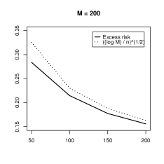
Figure 1: The excess risk of the ERM compared to $((\log M)/n)^{1/2}$ for several values of $M$ and $n$ ($x$-axis)

3.2 Aggregation

For each $f_{\lambda}\in F(\Lambda)$, we compute a weight $\theta(f_{\lambda})\in[0,1]$ such that $\sum_{\lambda\in\Lambda}\theta(f_{\lambda})=1$. These weights give a level of significance to each $f_{\lambda}\in F(\Lambda)$. The aggregated estimator is then the convex combination

$$\widehat{\mathsf{f}}:=\sum_{\lambda\in\Lambda}\theta(f_{\lambda})f_{\lambda},$$ (3.1)

where the weight of $f\in F(\Lambda)$ is given by

$$\theta(f):=\frac{\exp\big{(}-nR_{n}(f)/T\big{)}}{\sum_{\lambda\in\Lambda}\exp\big{(}-nR_{n}(f_{\lambda})/T\big{)}},$$ (3.2)

where $T>0$ is the so-called temperature parameter and where $R_{n}(f)$ is the empirical risk of $f$. This aggregation algorithm (with “Gibbs” or “exponential” weights) can also be found for instance in Catoni (2001); Leung and Barron (2006); Juditsky et al. (2005a, b); Yang (2000, 2004); Lecué (2007). See also Gaïffas and Lecué (2007) for adaptation by aggregation in a semiparametric model.

The next theorem is an oracle inequality for the aggregation method (3.2). It will be useful to derive the adaptive upper bounds stated in Section 4 below.

Theorem 4.

Assume that for any $f\in F(\Lambda)$, we have $\|f-f_{0}\|_{\infty}\leq Q$ for some $Q>0$. For any $a>0$, the aggregation method (3.2) satisfies

$$E^{n}\|\widehat{\mathsf{f}}-f_{0}\|^{2}\leq(1+a)\min_{f\in F(\Lambda)}\|f-f_{0}\|^{2}+(C+T)\frac{(\log n)^{1/2}\log M}{n},$$

where $C$ is a constant depending on $a,Q$ and $\sigma$.

When $T$ is too large, the weights (3.2) are close to the uniform law over the set of weak estimators, and of course, the resulting aggregate is inaccurate. When $T$ is too small, one weight is close to $1$, and the others close to $0$: in this situation, the aggregate does barely the same job as the ERM procedure. This is not suitable since Theorem 3 told us that ERM is suboptimal. Hence, $T$ realize a tradeoff between the ERM and the uniform weights procedure. It can be simply chosen by minimization of the empirical risk. We know empirically that it provides good results, see Gaïffas and Lecué (2007). Namely, we select the temperature

$$\widehat{T}:=\operatorname*{argmin}_{T\in\mathcal{T}}\sum_{i=1}^{n}\big{(}Y_{i}-\widehat{\mathsf{f}}^{(T)}(X_{i})\big{)}^{2},$$ (3.3)

where $\widehat{\mathsf{f}}^{(T)}$ is the aggregated estimator (3.1) with temperature $T$ and where $\mathcal{T}$ is some set of temperatures. This is what we do in the empirical study conducted in Section 5.

4 Examples of adaptive results

In this section, we construct adaptive estimators for several regression problems using the tools from Section 2 and 3. This involves, as usual with algorithms coming from statistical learning theory, a split of the sample into two parts (an exception can be found in Leung and Barron (2006)). The main steps of the construction of adaptive estimators given in this section are:

1. split, at random, the whole sample $D_{n}$ into a training sample

   $$D_{m}:=[(X_{i},Y_{i}):1\leq i\leq m],$$

   where $m<n$, and a learning sample

   $$D_{(m)}:=[(X_{i},Y_{i}):m+1\leq i\leq n];$$

2. choose a set $\Lambda$ of parameters and compute, using the training sample $D_{m}$, the corresponding class $F(\Lambda)=\{\bar{f}_{\lambda}:\lambda\in\Lambda\}$ of PERM (see Definition 1 in Section 2). Each $\Lambda$ depends on the considered problem of adaptive estimation, see below;

3. using the learning sample $D_{(m)}$, compute the aggregation weights and the aggregated estimator $\widehat{\mathsf{f}}_{n}$, respectively given by Equations (3.2) and (3.1).

Then, using Theorem 2 (see Section 2) and Theorem 3 (see Section 3), we will derive adaptive upper bounds for estimators $\widehat{\mathsf{f}}_{n}$ constructed in this way. Throughout the section, we shall assume the following.

Assumption (Split size).

Let $\ell$ be learning sample size, so that $\ell+m=n$. We shall assume from now on, to simplify the presentation, that $\ell$ is a fraction of $n$, typically $n/2$ or $n/4$.

4.1 About the split, jackknife

The behavior of the aggregate $\widehat{\mathsf{f}}_{n}$ can depend strongly on the split selected in Step 1, in particular when the number of observations is small. Hence, a good strategy is to jackknife: repeat, say, $J$ times Steps 1–3 to obtain aggregates $\{\widehat{\mathsf{f}}_{n}^{(1)},\ldots,\widehat{\mathsf{f}}_{n}^{(J)}\}$, and compute the mean:

$$\widehat{\mathsf{f}}_{n}:=\frac{1}{J}\sum_{j=1}^{J}\widehat{\mathsf{f}}_{n}^{(j)}.$$

This jackknifed estimator provides better results than a single aggregate, see Section 5 for an empirical study, where we show also that it gives more stable estimators than the ones involving cross-validation of generalized cross-validation. By convexity of $f\mapsto\|f-f_{0}\|^{2}$, the jackknifed estimator satisfies the same upper bounds as a single aggregate: each of the adaptive upper bounds stated below also holds when we use the jackknife.

For the set of weak estimators considered in this paper, the split of the data is not a theoretical artefact. Indeed, if one skips Step 1 (compute $F(\Lambda)$ and $\widehat{\mathsf{f}}_{n}$ using the whole sample $D_{n}$), then $\widehat{\mathsf{f}}_{n}$ has a very poor performance. An empirical illustration of this phenomenon is given in Figure 2. Herein, we show the aggregation weights (3.2) when the data is splitted and when it is not splitted. We consider an univariate design and cubic smoothing splines. Namely, we compute the set $F(\Lambda)$ of PERM (see (2.1)) with $\mathcal{F}=\{f\in L^{2}([0,1]):\int f^{(2)}(t)dt<+\infty\}$ and penalty $\operatorname{pen}(f)=h^{2}\int f^{(2)}(t)dt$, where $f^{(2)}$ stands for the second derivative of $f$. We do that for several smoothing parameters $h$ in a grid $H$, so that $\Lambda:=\{(h,\mathcal{F}):h\in H\}$. We used the smooth.spline routine in the R software to compute $F(\Lambda)$.

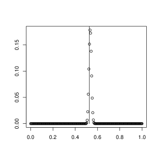
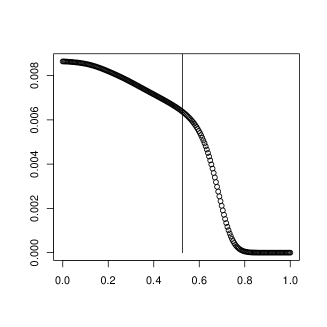
Figure 2: Aggregation weights with split (left) and without split (right) and smoothing parameter obtained by cross-validation (vertical line)

In Figure 2, the x-axis is related to the value of $h$: it is the value of the parameter spar from the smooth.spline routine. The vertical line is the value of spar selected by cross-validation. The conclusion from Figure 2 is that, when the data is not splitted, an overfitting phenomenon occurs: the aggregation algorithm does not work, since it does not concentrate around a value of spar. Of course, the resulting aggregated estimator has a very poor performance.

4.2 How to derive the adaptive upper bounds

In every examples considered below, the scheme to derive adaptive upper bounds is as follows. Say that $(\mathcal{F}_{\beta}:\beta\in B)$ is a set of embedded functions classes ($\mathcal{F}_{\beta}\subset\mathcal{F}_{\beta^{\prime}}$ if $\beta<\beta^{\prime}$) where each $\mathcal{F}_{\beta}$ satisfy Assumption $(C_{\beta})$. Let $B_{n}$ be an appropriate discretization of $B$. Let $\widehat{\mathsf{f}}_{n}$ be the aggregated estimator obtained using Steps 1–3 (see the beginning of the section), with parameter $\Lambda=\Lambda_{n}=\{(n^{-2/(2+\beta)},\mathcal{F}_{\beta}):\beta\in B_{n}\}$ and let $M_{n}$ be the cardinality of $F(\Lambda_{n})$. Let $E^{m}$ and $E^{(m)}$ be the expectations with respect to, repectively, the joint laws of $D_{m}$ and $D_{(m)}$, so that, by independence, we have $E^{n}[\cdot]=E^{m}[E^{(m)}[\cdot]]$. Let $f_{0}\in\mathcal{F}_{\beta_{0}}$ for some $\beta_{0}\in B$. Using Theorem 4, we have

$$E^{(m)}\|\widehat{\mathsf{f}}_{n}-f_{0}\|^{2} \leq C\min_{f\in F(\Lambda_{n})}\|f-f_{0}\|^{2}+\frac{C(\log n)^{1/2}\log M_{n}}{n}$$

$$\leq C\|\bar{f}_{\lambda_{n}}-f_{0}\|^{2}+\frac{C(\log n)^{1/2}\log M_{n}}{n},$$

where $\lambda_{n}=(n^{-2/(2+\beta_{n})},\mathcal{F}_{\beta_{n}})$, with $\beta_{n}\in B_{n}$ chosen such that $\mathcal{F}_{\beta_{0}}\subset\mathcal{F}_{\beta_{n}}$ and $n^{-2/(2+\beta_{n})}\leq C_{1}n^{-2/(2+\beta_{0})}$. Then, integrating w.r.t. to $E^{m}$ and using Theorem 2, we have, if $M_{n}$ is no more than a power of $n$:

$$E^{n}\|\widehat{\mathsf{f}}_{n}-f_{0}\|^{2} \leq CE^{m}\|\bar{f}_{\lambda_{n}}-f_{0}\|^{2}+o(n^{-2/(2+\beta_{0})})$$

$$\leq C_{2}n^{-2/(2+\beta_{n})}+o(n^{-2/(2+\beta_{0})})\leq C_{3}n^{-2/(2+\beta_{0})}.$$

This prove that, if $f_{0}\in\mathcal{F}_{\beta_{0}}$ for some $\beta_{0}\in B$, we have $E^{n}\|\widehat{\mathsf{f}}_{n}-f_{0}\|^{2}\leq C_{3}n^{-2/(2+\beta_{0})}$, thus $\widehat{\mathsf{f}}_{n}$ is indeed adaptive over $(\mathcal{F}_{\beta}:\beta\in B)$.

4.3 Sobolev spaces, spline estimators

When $\mathcal{F}$ is a Sobolev space, the PERM (2.1) with $\alpha=2$ is a very popular smoothing technique: see, among others, Wahba (1990) and Green and Silverman (1994). The most simple example is when $d=1$ and

$$\mathcal{F}=W_{2}^{s}([0,1]):=\Big{\{}f\in L^{2}([0,1]):|f|_{W_{2}^{s}}^{2}:=\int_{0}^{1}f^{(s)}(t)^{2}dt<\infty\Big{\}},$$

where $s$ is some natural integer and $f^{(s)}$ stands for the $s$-th derivative of $f$. In this case, the PERM is called a smoothing spline, since in this situation the unique minimizer of (2.1) is a spline, see for instance Wahba (1990) or Györfi et al. (2002). When $s=2$ (cubic splines), the routine smooth.spline from the R software (and for other softwares as well) neatly computes the solution to (2.1) using the B-spline basis, and chooses the parameter $h$ via generalized cross-validation (GCV).

The $d$-dimensional case is easily understood with the definition of $W_{2}^{s}([0,1]^{d})$ as the space of functions $f\in L^{2}([0,1]^{d})$ with all derivatives of total order $s$ in $L^{2}([0,1]^{d})$. Namely,

$$W_{2}^{s}([0,1]^{d}):=\Big{\{}f\in L^{2}([0,1]^{d}):|f|_{W_{2}^{s}([0,1]^{d})}^{2}<\infty\Big{\}},$$

where

$$|f|_{W_{2}^{s}([0,1]^{d})}^{2}:=\sum_{\mathbf{k}\in\mathbb{N}_{0}^{d}:|\mathbf{k}|=s}\frac{s!}{\mathbf{k}!}\int_{[0,1]^{d}}(D_{\mathbf{k}}f(x))^{2}dx,$$ (4.1)

where for $\mathbf{k}=(k_{1},\ldots,k_{d})$ we use the notations $\mathbf{k}!:=\prod_{i=1}^{d}k_{i}!$ and $|\mathbf{k}|:=\sum_{i=1}^{d}k_{i}$ and where $D_{\mathbf{k}}$ is the differential operator $\partial^{s}/(\partial^{k_{1}}\cdots\partial^{k_{d}})$. When $d>1$, the PERM for the choice $\mathcal{F}=W_{2}^{s}([0,1]^{d})$ is called a thin plate spline, see again for instance Wahba (1990) or Györfi et al. (2002), where the practical computation of such PERM is explained in details. The usual assumption $s>d/2$ gives the embedding $W_{s}([0,1]^{d})\subset C[0,1]^{d}$ and that Assumption $(C_{\beta})$ holds, see Birman and Solomjak (1967). The situation where $s$ is not an integer is a particular case of what we do in Section 4.5 below. The case where $\mathcal{F}$ is a Sobolev space is actually a particular case of both the next sections. Indeed, it is well known (see Wahba (1990) for instance) that a Sobolev space is a Reproductive Kernel Hilbert Space (RKHS) for an appropriate kernel choice, and that it is also a Besov space $B_{2,2}^{s}$.

4.4 Reproductive Kernel Hilbert Spaces

Reproductive Kernel Hilbert Spaces (cf. Aronszajn (1950)), RKHS for short, provide a unified context for regularization in a wide variety of statistical model. Computational properties of estimators obtained by minimization of a functional onto a RKHS make these functions space very useful for statisticians. In this short section, we briefly recall some definitions and computational properties of RKHS.

Let ${\cal X}$ be an abstract space (in this paper, we take ${\cal X}=[0,1]^{d}$). We say that $K:{\cal X}\times{\cal X}\longmapsto\mathbb{R}$ is a reproducing kernel, RK for short, if for any integer $p$ and any points $x_{1},\ldots,x_{p}$ in ${\cal X}$, the matrix $(K(x_{i},x_{j}))_{1\leq i,j\leq p}$ is symmetric positive definite. Let $K$ be a RK. The Hilbert space associated with $K$, called Reproducing Kernel Hilbert Space and denoted by ${\cal H}_{K}$, is the completion of the space of all the finite linear combination $\sum_{j}a_{j}K(x_{j},\cdot)$ endowed with the inner product $\langle\sum_{j}a_{j}K(x_{j},\cdot),\sum_{k}b_{k}K(y_{k},\cdot)\rangle_{K}=\sum_{j,k}a_{j}b_{k}K(x_{j},y_{k})$. We denote by $|\cdot|_{K}$ the associated norm on ${\cal H}_{K}$.

The representer theorem (see Kimeldorf and Wahba (1971) for results on optimization in RKHS) is at the heart of minimization of functional onto RKHS. The solution of the minimization problem

$$\bar{f}\in\operatorname*{argmin}_{f\in{\cal H}_{K}}\{R_{n}(f)+h^{2}|f|_{{\cal H}_{K}}^{2}\}$$ (4.2)

is the linear combination

$$\bar{f}(\cdot)=\sum_{i=1}^{n}\alpha_{i}K(X_{i},\cdot),\mbox{ where }\boldsymbol{\alpha}=(\alpha_{i})_{1\leq i\leq n}=(\mathbf{K}_{X}+nh^{2}\mathbf{I}_{n})^{-1}\mathbf{Y},$$

where $\mathbf{K}_{X}$ is the Gram matrix $(K(X_{i},X_{j}))_{1\leq i,j\leq n}$, where $\mathbf{Y}=(Y_{1},\ldots,Y_{n})$ and where $\mathbf{I}_{n}$ is the identity matrix in $\mathbb{R}^{n}$. They are many different ways to simplify the computation of the coefficients $\boldsymbol{\alpha}$, see for instance Amato et al. (2006).

In order to derive convergence rates for the estimator defined in (4.2) from Theorem 2, we use some results about covering numbers of RKHS obtained in Cucker and Smale (2002) (other results on the entropy of RKHS can be found in Steinwart and Scovel (2007); Carl and Stephani (1990)). Let now assume that $P_{X}$ is a Borel measure. If $K$ is a Mercer kernel (this is a continuous reproducing kernel), the RKHS associated with $K$ is the set

$${\cal H}_{K}=\Big{\{}f\in L_{2}(P_{X}):f=\sum_{j=1}^{\infty}a_{j}\psi_{j}\mbox{ s.t. }\sum_{j=1}^{\infty}\lambda_{j}^{-1}a_{j}^{2}\leq\infty\Big{\}},$$

where $(\lambda_{j})_{j\geq 1}$ is the sequence of decreasing eigenvalues of the operator

$$L_{K}:\left\{\begin{array}[]{ccc}L^{2}(P_{X})&\longrightarrow&L^{2}(P_{X})\\ f&\longmapsto&\int_{\cal X}K(\cdot,y)f(y)dP_{X}(y)\end{array}\right.$$

and $(\psi_{j})_{j\leq 1}$ the sequence of corresponding eigenvectors. According to Proposition 9 and Theorem D in Cucker and Smale (2002), if for any $k\geq 1$ the $k$-th eigenvalue of $L_{K}$ is such that

$$\lambda_{k}\leq Ck^{-l}$$ (4.3)

for some $C>0$ and $l>1/2$ then the entropy of $B_{K}(R):=\{f\in{\cal H}_{K}:|f|_{K}\leq R\}$ satisfies for any $\delta>0$:

$$H_{\infty}(\delta,B_{K}(R))\leq\Big{(}\frac{2RC_{l}}{\delta}\Big{)}^{1/l},$$

where $C_{l}$ is slightly greater than $6Cl^{l}$. In this case, Theorem 2 and the arguments from Section 4.2 gives the following result.

Corollary 1 (Adaptive upper bound for RKHS).

Let $\bar{f}$ be defined by (4.2) with a reproducing kernel $K$ such that the eigenvalues of the operator $L_{K}$ satisfy (4.3). Then, if $h=an^{-l/(2l+1)}$ and $\|\bar{f}-f_{0}\|_{\infty}\leq Q$, we have

$$E^{n}\|\bar{f}-f_{0}\|_{L^{2}(P_{X})}^{2}\leq C_{2}(1+|f_{0}|^{2}_{\mathcal{H}_{K}})n^{-2l/(2l+1)}$$

when $n$ is large enough.

Now, let $L=[l_{\min},l_{\max}]$ where $l_{\min}>1/2$ and $(\mathcal{H}_{l}:l\in L)$ be a family of nested RKHS. Assume that the kernel of each $\mathcal{H}_{l}$ satisfies (4.3). Let $\widehat{\mathsf{f}}_{n}$ be the aggregated estimator defined by Steps 1-3 with $\Lambda_{n}=\{\lambda=(n^{-l/(2l+1)},\mathcal{H}_{l}):l\in L_{n}\}$ and $L_{n}:=\{l_{\min},l_{\min}+(\log n)^{-1},\ldots,l_{\max}\}$. We have, if $f_{0}\in\mathcal{H}_{l}$ for some $l\in L$,

$$E^{n}\|\widehat{\mathsf{f}}_{n}-f_{0}\|_{L^{2}(P_{X})}^{2}\leq C_{2}(1+|f_{0}|^{2}_{\mathcal{H}_{l}})n^{-2l/(2l+1)}$$

when $n$ is large enough.

4.5 Anisotropic Besov spaces

In nonparametric estimation literature, Besov spaces are of particular interest since they include functions with inhomogeneous smoothness, for instance functions with rapid oscillations or bumps. Roughly, these spaces are used in statistics when we want to prove theoretically that some adaptive estimator is able to recover the details of a functions. When one considers a multivariate regression, the question of anisotropic smoothness naturally arises. Anisotropy means that the smoothness of $f_{0}$ differs in function of coordinates. As far as we know, adaptive estimation of a multivariate curve with anisotropic smoothness was previously considered only in Gaussian white noise or density models, see Hoffmann and Lepski (2002), Kerkyacharian et al. (2001), Kerkyacharian et al. (2007), Neumann (2000). There is no results concerning the adaptive estimation of the regression with anisotropic smoothness on a general random design.

In this Section, we construct, using Steps 1-3, an adaptive estimator over anisotropic Besov spaces $B_{p,q}^{\boldsymbol{s}}$, where $\boldsymbol{s}=(s_{1},\ldots,s_{d})$ is the vector of smoothnesses. If $\{e_{1},\ldots,e_{d}\}$ is the canonical basis of $\mathbb{R}^{d}$, each $s_{i}$ is the smoothness in the direction $e_{i}$. A precise definition of $B_{p,q}^{\boldsymbol{s}}$ is given in Appendix A. Let $s$ be the harmonic mean of $\boldsymbol{s}$, see (2.3). Let us introduce two vectors $\boldsymbol{s}^{\min}$ and $\boldsymbol{s}^{\max}$ in $\mathbb{R}_{+}^{d}$ with positive coordinates and harmonic means $\bar{\boldsymbol{s}}^{\min}$ and $\bar{\boldsymbol{s}}^{\max}$ respectively. Assume that $\boldsymbol{s}^{\min}\leq{\boldsymbol{s}}^{\max}$, which means that $s_{i}^{\min}\leq s_{i}^{\max}$ for any $i\in\{1,\ldots,d\}$ and assume that $\bar{\boldsymbol{s}}^{\min}>d/\min(p,2)$. In view of Theorem 5 and the embedding (A.1) (see Appendix A), we know that Assumption $(C_{\beta})$ holds for every $B_{p,\infty}^{\boldsymbol{s}}$ such that $\boldsymbol{s}\geq\boldsymbol{s}^{\min}$ with $\beta=d/\bar{\boldsymbol{s}}$ (and every $B_{p,q}^{\boldsymbol{s}}$, since $B_{p,q}^{\boldsymbol{s}}\subset B_{p,\infty}^{\boldsymbol{s}}$), where $\bar{\boldsymbol{s}}$ is the harmonic mean of $\boldsymbol{s}$. Consider the “cube of smoothness”

$$\boldsymbol{S}:=\prod_{i=1}^{d}[s_{i}^{\min},s_{i}^{\max}],$$ (4.4)

and consider the uniform discretization of this cube with step $(\log n)^{-1}$:

$$\boldsymbol{S}_{n}:=\prod_{i=1}^{d}\big{\{}s_{i}^{\min}+k(\log n)^{-1}:1\leq k\leq[(s_{i}^{\max}-s_{i}^{\min})\log n]\big{\}},$$ (4.5)

and the set of parameters

$$\Lambda(\boldsymbol{S}):=\{\lambda=(n^{-\bar{\boldsymbol{s}}/(2\bar{\boldsymbol{s}}+d)},B_{p,q}^{\boldsymbol{s}}):\boldsymbol{s}\in\boldsymbol{S}_{n}\}.$$

Now, we compute, following Steps 1-3, the aggregated estimator $\widehat{\mathsf{f}}_{n}^{\boldsymbol{S}}$ with set of parameters $\Lambda(\boldsymbol{S})$ (see the beginning of the section). Following the arguments from Section 4.2, we can prove in the following Corollary 2 that $\widehat{\mathsf{f}}_{n}^{\boldsymbol{S}}$ is adaptive over the whole range of anisotropic Besov spaces $\{B_{p,q}^{\boldsymbol{s}}:\boldsymbol{s}\in\boldsymbol{S}\}$.

Corollary 2.

Assume that $\|\bar{f}-f_{0}\|_{\infty}\leq Q$ for every $\bar{f}\in F(\boldsymbol{S})$. If $f_{0}\in B_{p,q}^{\boldsymbol{s}}$ for some $s\in\boldsymbol{S}$, then

$$E^{n}\|\widehat{\mathsf{f}}_{n}^{\boldsymbol{S}}-f_{0}\|_{L^{2}(P_{X})}^{2}\leq Cn^{-2\bar{\boldsymbol{s}}/(2\bar{\boldsymbol{s}}+d)}$$

when $n$ is large enough, where $C$ is a constant depending on $\boldsymbol{S},d$ and $Q$.

In Corollary 2 we recover the “expected” minimax rate $n^{-2\bar{\boldsymbol{s}}/(2\bar{\boldsymbol{s}}+d)}$ of estimation of a $d$-dimensional curve in a Besov space. Note that there is no regular or sparse zone here, since the error of estimation is measured with $L^{2}(P_{X})$ norm. A minimax lower bound over $B_{p,q}^{\boldsymbol{s}}$ can be easily obtained using standard arguments, such as the ones from Tsybakov (2003a), together with Bernstein estimates over $B_{p,q}^{\boldsymbol{s}}$ that can be found in Hochmuth (2002). Note that the only assumption required on the design law in this corollary is the compactness of its support.

5 Empirical study

In this Section, we compare empirically our aggregation procedure with the popular cross-validation (CV) and generalized cross-validation (GCV) procedures for the selection of the smoothing parameter $h$ (see Section 2.5) in smoothing splines (we use the smooth.spline routine from the R software, see http://www.r-project.org/). Concerning CV, GCV and smoothing splines, we refer to Wahba (1990) and Green and Silverman (1994). Those routines provide satisfactory results in most cases, in particular for the examples of regression functions considered here. However, we show that when the sample size $n$ is small (less than 50), and when the noise level is high (we take root-signal-to-noise ratio equals to $2$), then our aggregation approach is more stable, see Figure 4 below. Here in, we consider two examples of regression function, given, for $x\in[-1,1]$, by:

• hardsine$(x)=2\sin(1+x)\sin(2\pi x^{2}+1)$

• oscsine$(x)=(x+1)\sin(4\pi x^{2})$.

We simply take $X$ uniformly distributed on $[-1,1]$ and Gaussian noise with variance $\sigma$ chosen so that the root-signal-to-noise ratio is $2$. In Figure 3 we show typical simulation in this setting, where $n=30$.

Figure 3: Examples of simulated data, for $f_{0}$=harsine (left) and $f_{0}$=oscsine (right)

In Figure 4, we show the mises $E\|\widehat{f}_{n}-f_{0}\|_{n}^{2}$ computed by Monte Carlo using $1000$ simulations of the model. The tuning of the estimators in both examples is the following: for GCV, we simply use the smooth.spline routine with default selection of $h$ by GCV. For CV, we use the same routine, with the option cv=TRUE so that CV is used instead. For aggregation, we use Steps 1-3 (see Section 4). Step 1 is done with $m=3n/4$ and $\ell=n/4$. For Step 2, we use the smooth.spline routine to compute a set of weak estimators, using the option spar=x, where x lies in the set $\{0,0.01,0.02\ldots,1\}$. The parameter spar is related to the value of the smoothing parameter $h$. For Step 3, we compute the weights with temperature given by (3.3) (over the training sample) and the set $\mathcal{T}=\{10,20,\ldots,100\}$. Then, we repeat steps 1-3 $J=100$ times and compute the jackknifed estimator, see Section 4.1. This gives our aggregated estimator.

On Figure 4, we plot the MISEs (the mean of the $1000$ MISEs obtained for each simulation) for sample sizes $n\in\{20,30,50,100\}$ and in Figure 5 we plot the corresponding standard deviations. The conclusion is that for small $n$, aggregation provides a more accurate and stable estimation than the GCV or CV. When $n$ is $100$ or larger, than the aggregation procedure has barely the same accuracy as GCV or CV.

Figure 4: MISE for $f_{0}$=harsine (left) and $f_{0}$=oscsine (right)

Figure 5: standard deviation of the MISE for $f_{0}$=harsine (left) and $f_{0}$=oscsine (right)

6 Proofs of the main results

We recall that $P_{n}$ stands for the joint law of the training sample $D_{n}$ conditional on $X^{n}:=(X_{1},\ldots,X_{n})$, that is $P_{n}:=P^{n}[\cdot|X^{n}]$.

Proof of Theorem 1.

First, we use the peeling argument: we decompose $B_{n}(f_{0},\delta)$ into the union of the sets $S_{j}$ for $j\geq 0$, where for $\delta_{j}:=\delta 2^{-j/\beta}$

$$S_{j}:=B_{n}(f_{0},\delta_{j})-B_{n}(f_{0},\delta_{j+1}),$$

and decompose $\mathcal{F}$ into the union of the sets

$$B_{\cal F}(2^{k/\beta})-B_{\cal F}(2^{(k-1)/\beta})=\{f\in\mathcal{F}:2^{(k-1)/\beta}<|f|_{\mathcal{F}}\leq 2^{k/\beta}\},$$

for $k\geq 1$, where $B_{\mathcal{F}}(2^{k/\beta})=\{f\in\mathcal{F}:|f|_{\mathcal{F}}\leq 2^{k/\beta}\}$ This gives that the left hand side of (2.6) is smaller than

$$\sum_{j\geq 0} P_{n}\Big{[}\sup_{\begin{subarray}{c}f\in S_{j}\text{ s.t. }\\ |f|_{\mathcal{F}}\leq 1\end{subarray}}\frac{Z(f-f_{0})}{\|f-f_{0}\|_{n}^{1-\beta/2}(1+|f|_{\mathcal{F}})^{\beta/2}}>z\Big{]}$$

$$+\sum_{j\geq 0}\sum_{k\geq 1}P_{n}\Big{[}\sup_{f\in S_{j}\cap B_{\mathcal{F}}(2^{k/\beta})}\frac{Z(f-f_{0})}{\|f-f_{0}\|_{n}^{1-\beta/2}(1+|f|_{\mathcal{F}})^{\beta/2}}>z\Big{]},$$

which is smaller than

$$\sum_{j,k\geq 0}P_{n}\Big{[}\sup_{f\in B_{n}(f_{0},\delta_{j})\cap B_{\cal F}(2^{k/\beta})}Z(f-f_{0})>z(\delta,j,k)\Big{]}=:\sum_{j,k\geq 0}P_{j,k},$$

where $z(\delta,j,k):=z\delta_{j}^{1-\beta/2}2^{k/2-1/2}$. Let us consider, for any $\delta>0$, a minimal $\delta$-covering $F(\delta,k)$ of the set $B_{\mathcal{F}}(2^{k/\beta})$ for the $\|\cdot\|_{\infty}$-norm. Assumption $(C_{\beta})$ implies

$$|F(\delta,k)|\leq\exp\big{(}D(2^{k/\beta}/\delta)^{\beta}\big{)}=\exp(D2^{k}\delta^{-\beta}).$$

Moreover, without loss of generality, we can assume that $F(\delta,k)\subset B_{\mathcal{F}}(2^{k/\beta})$. For any $i\in\mathbb{N}$ and $j,k$ fixed, we introduce

$$F^{(i)}:=F(\delta_{i,j},k)\text{ where }\delta_{i,j}:=\delta_{j}2^{-i/\beta}=\delta 2^{-(i+j)/\beta},$$ (6.1)

and, for any $f\in B_{\cal F}(2^{k/\beta})$ we denote by $\pi_{i}(f)$ an element of $F^{(i)}$ such that $\|\pi_{i}(f)-f\|_{\infty}\leq\delta_{i,j}$. We have

$$P_{j,k} \leq P_{n}\Big{[}\sup_{f\in B_{n}(f_{0},\delta_{j})\cap B_{\cal F}(2^{k/\beta})}|Z(\pi_{0}(f)-f_{0})|>z(\delta,j,k)/2\Big{]}$$

$$+P_{n}\Big{[}\sup_{f\in B_{n}(f_{0},\delta_{j})\cap B_{\cal F}(2^{k/\beta})}|Z(f-\pi_{0}(f))|>z(\delta,j,k)/2\Big{]}$$

$$=:P_{j,k,1}+P_{j,k,2}.$$

First, we consider $P_{j,k,1}$:

$$P_{j,k,1}\leq P_{n}\Big{[}\sup_{f\in F^{(0)}\cap B_{n}(f_{0},\delta_{j})}|Z(\pi_{0}(f)-f_{0})|>z(\delta,j,k)/2\Big{]}.$$

We use (2.5) and the union bound over $F^{(0)}$ together with the fact that $f\in B_{n}(f_{0},\delta_{j})$ to obtain:

$$P_{j,k,1}\leq|F^{(0)}|\exp\Big{(}\frac{-az^{2}(\delta,j,k)}{4\delta_{j}^{2}}\Big{)}=\exp\Big{(}\frac{2^{j+k}}{\delta^{\beta}}(D-az^{2}/8)\Big{)},$$

where $a:=(2b^{2})^{-1}$. Now, in order to control $P_{j,k,2}$, we use the so-called chaining argument, which involves increasing approximations by the covers $F^{(i)}$, see (6.1). Let us consider

$$E_{i}:=(2^{1/\beta-1/2}-1)2^{-i(1/\beta-1/2)}$$

for $i\geq 1$ ($E_{i}>0$ since $\beta\in(0,2)$). By linearity of $Z_{n}(\cdot)$ and since $\sum_{i\geq 1}E_{i}=1$, we have

$$P_{j,k,2} \leq\sum_{i\geq 1}P_{n}\Big{[}\sup_{\begin{subarray}{c}f\in B_{n}(f_{0},\delta_{j})\\ |f|_{\mathcal{F}}\leq 2^{k/\beta}\end{subarray}}|Z(\pi_{i}(f)-\pi_{i-1}(f))|>E_{i}z(\delta,j,k)/2\Big{]}$$

$$=:\sum_{i\geq 1}P_{i,j,k,2}.$$

Now, since

$$\|\pi_{i}(f)-\pi_{i-1}(f)\|_{n} \leq\|\pi_{i}(f)-\pi_{i-1}(f)\|_{\infty}$$

$$\leq\|\pi_{i}(f)-f\|_{\infty}+\|\pi_{i-1}(f)-f\|_{\infty}$$

$$\leq\delta_{i,j}+\delta_{i-1,j}=\delta_{i,j}(1+2^{1/\beta}),$$

and since the number of pairs $\{\pi_{i}(f),\pi_{i-1}(f)\}$ is at most

$$|F^{(i)}|\times|F^{(i-1)}|\leq\exp\Big{(}\frac{3D2^{i+j+k}}{2\delta^{\beta}}\Big{)},$$

we obtain using again (2.5):

$$P_{i,j,k,2} \leq|F^{(i)}|\times|F^{(i-1)}|\times\exp\Big{(}\frac{-aE_{i}^{2}z^{2}(\delta,j,k)}{4\delta_{i,j}^{2}(1+2^{1/\beta})^{2}}\Big{)}$$

$$=\exp\Big{(}\frac{2^{i+j+k}}{\delta^{\beta}}\big{(}3D/2-C_{1}z^{2}\big{)}\Big{)}$$

where $C_{1}=C_{1}(s,d,a):=a(2^{1/\beta-1/2}-1)/(8(1+2^{1/\beta})^{2})>0$. Then, if we choose $z_{1}:=(3/C_{1})^{1/2}$, we have for any $z\geq z_{1}$ and $D_{1}:=C_{1}/2$:

$$\sum_{j,k\geq 0}P_{j,k} \leq\sum_{j,k\geq 0}\Big{(}P_{j,k,1}+\sum_{i\geq 1}P_{i,j,k,2}\Big{)}$$

$$\leq\sum_{j,k\geq 0}\Big{(}\exp(-D_{1}2^{j+k}z^{2}\delta^{-\beta})+\sum_{i\geq 1}\exp(-D_{1}2^{i+j+k}z^{2}\delta^{-\beta})\Big{)}$$

and the Theorem follows. ∎

Proof of Theorem 2.

For short, we shall write $\bar{f}$ instead of $\bar{f}_{\lambda}$, and $\operatorname{pen}(f)$ instead of $\operatorname{pen}_{\lambda}(f)$. In view of (2.1), we have

$$\|Y-\bar{f}\|_{n}^{2}+\operatorname{pen}(\bar{f})\leq\|Y-f\|_{n}^{2}+\operatorname{pen}(f)\quad\forall f\in\mathcal{F},$$ (6.2)

which is equivalent to

$$\|\bar{f}-f\|_{n}^{2}+\operatorname{pen}(\bar{f})\leq 2\langle Y-f,\bar{f}-f\rangle_{n}+\operatorname{pen}(f)\quad\forall f\in\mathcal{F},$$

where $\langle f,g\rangle_{n}=n^{-1}\sum_{i=1}^{n}f(X_{i})g(X_{i})$. This entails, since $f_{0}\in\mathcal{F}$, that

$$\|\bar{f}-f_{0}\|_{n}^{2}+\operatorname{pen}(\bar{f})\leq\frac{2}{\sqrt{n}}Z(\bar{f}-f_{0})+\operatorname{pen}(f_{0})$$ (6.3)

where $Z(\cdot)$ is the empirical process given by (2.4). Recall that $B_{n}(f_{0},\delta)$ stands for the ball centered at $f_{0}$ with radius $\delta$ for the norm $\|\cdot\|_{n}$. Let us introduce the event

$$\mathcal{Z}(z,\delta):=\Big{\{}\sup_{f\in\mathcal{F}\cap B_{n}(f_{0},\delta)}\frac{Z(f-f_{0})}{\|f-f_{0}\|_{n}^{1-\beta/2}(1+|f|_{\mathcal{F}})^{\beta/2}}\leq z\Big{\}}.$$ (6.4)

In view of Theorem 1, see Section 2.3, we can find constants $z_{1}>0$ and $D_{1}>0$ such that:

$$P_{n}\big{[}\mathcal{Z}(z,\delta)^{\complement}\big{]}\leq\exp(-D_{1}z^{2}\delta^{-\beta}),$$

for any $\delta>0$ and $z\geq z_{1}$. When $2n^{-1/2}Z(\bar{f}-f_{0})\leq\operatorname{pen}(f_{0})$, we have $\|\bar{f}-f_{0}\|_{n}^{2}\leq 2\operatorname{pen}(f_{0})$. When $2n^{-1/2}Z(\bar{f}-f_{0})\geq\operatorname{pen}(f_{0})$, we have, for any $z>0$, in view of (6.3), whenever $\bar{f}\in B_{n}(f_{0},\delta)$ for some $\delta>0$, that on $\mathcal{Z}(z,\delta)$,

$$\|\bar{f}-f_{0}\|_{n}^{2}+\operatorname{pen}(\bar{f})\leq\frac{4z}{\sqrt{n}}\|\bar{f}-f_{0}\|_{n}^{1-\beta/2}(1+|\bar{f}|_{\mathcal{F}})^{\beta/2}.$$

If $|\bar{f}|_{\mathcal{F}}\leq 1$, this entails

$$\|\bar{f}-f_{0}\|_{n}^{2}+\operatorname{pen}(\bar{f})\leq(a^{-2}(2^{\beta}4z)^{4/(2+\beta)}+1)h^{2}.$$

Otherwise, we have

$$\|\bar{f}-f_{0}\|_{n}^{2}+\operatorname{pen}(\bar{f})\leq\frac{2^{\beta/2}4z}{\sqrt{n}}\|\bar{f}-f_{0}\|_{n}^{1-\beta/2}|\bar{f}|_{\mathcal{F}}^{\beta/2},$$

and we use the following lemma.

Lemma 1.

Let $r,I,h,\varepsilon$ be positive numbers, $\beta\in(0,2)$ and $\alpha>2\beta/(\beta+2)$. Then, if

$$r^{2}+h^{2}I^{\alpha}\leq\varepsilon\,r^{1-\beta/2}I^{\beta/2},$$ (6.5)

we have

$$r\leq(\varepsilon^{\alpha}h^{-\beta})^{2/(2\alpha+\alpha\beta-2\beta)},\quad I\leq(\varepsilon^{2}h^{-(\beta+2)})^{2/(2\alpha+\alpha\beta-2\beta)}$$

and consequently

$$r^{2}+h^{2}I^{\alpha}\leq 2(\varepsilon^{\alpha}h^{-\beta})^{4/(2\alpha+\alpha\beta-2\beta)}.$$

The proof of this Lemma is given in Section 7 below. It entails, since $h=an^{-1/(2+\beta)}$ and $\alpha>2\beta/(\beta+2)$, that

$$\|\bar{f}-f_{0}\|_{n}^{2}+h^{2}|\bar{f}|_{\mathcal{F}}^{\alpha}\leq 2((2^{\beta/2}4z)^{\alpha}a^{-\beta})^{4/(2\alpha+\alpha\beta-2\beta)}n^{-2/(\beta+2)}.$$

Thus, when $\bar{f}\in B_{n}(f_{0},\delta)$, we have on $\mathcal{Z}(z,\delta)$:

$$\|\bar{f}-f_{0}\|_{n}^{2}+\operatorname{pen}(\bar{f})\leq p(z)^{2}h^{2}$$

where

$$p(z)^{2}:=C_{1}(1+z^{4/(2+\beta)}+z^{4\alpha/(2\alpha+\alpha\beta-2\beta)})$$

and $C_{1}$ is a constant depending on $\alpha,\beta$ and $a$. Let us assume for now that $\|\bar{f}-f_{0}\|_{n}\leq\delta$ for some $\delta>0$, and let us introduce

$$\mathcal{Z}_{1}(z,\delta):=\mathcal{Z}(z,\delta)\cap\mathcal{Z}(z_{1},p(z)h),$$

where $z_{1}$ is a constant coming from Theorem 1. On $\mathcal{Z}_{1}(z,\delta)$, we have

$$\|\bar{f}-f_{0}\|_{n}^{2}+\operatorname{pen}(\bar{f})\leq p(z_{1})^{2}h^{2}.$$ (6.6)

Indeed, we have $\bar{f}\in B_{n}(f_{0},\delta)$ thus, on $\mathcal{Z}(z,\delta)$, $\|\bar{f}-f_{0}\|_{n}^{2}+\operatorname{pen}(\bar{f})\leq p(z_{1})^{2}h^{2}$ and so $\|\bar{f}-f_{0}\|_{n}^{2}\leq p(z)^{2}h^{2}$. Thus, on the event $\mathcal{Z}(z_{1},p(z)h)$, we have (6.6). Moreover, Theorem 1 yields

$$P_{n}\big{[}\mathcal{Z}_{1}(z,\delta)^{\complement}\big{]}\leq\exp(-D_{1}z^{2}\delta^{-\beta})+\exp(-D_{1}z_{1}^{2}(p(z)h)^{-\beta}).$$ (6.7)

Now, in view of (6.2) and since $f_{0}\in\mathcal{F}$, we have the following rough majoration:

$$\|\bar{f}-f_{0}\|_{n}^{2}+\operatorname{pen}(\bar{f}) \leq 2(\|\bar{f}-Y\|^{2}_{n}+\operatorname{pen}(\bar{f}))+2\|f_{0}-Y\|_{n}^{2}$$

$$\leq 2(\|f_{0}-Y\|_{n}^{2}+\operatorname{pen}(f_{0}))+2\|f_{0}-Y\|_{n}^{2}$$

$$\leq 4\sigma^{2}\|\varepsilon\|_{n}^{2}+2\operatorname{pen}(f_{0}),$$ (6.8)

which entails

$$E_{n}\big{[}\big{(}\|\bar{f}-f_{0}\|_{n}^{2}+\operatorname{pen}(\bar{f})\big{)}^{2}\big{]}\leq\sigma^{4}C(\varepsilon)^{2}+8h^{4}|f_{0}|_{\mathcal{F}}^{2\alpha}$$

where $C(\varepsilon)^{2}=32(E[\varepsilon^{4}]/n+2(E[\varepsilon^{2}])^{2})$. Putting all this together, we obtain, by a decomposition of $E_{n}[\|\bar{f}-f_{0}\|_{n}^{2}+\operatorname{pen}(\bar{f})]$ over the union of the sets $\{\|\bar{f}-f_{0}\|_{n}\leq\delta\}\cap\mathcal{Z}_{1}(z,\delta)$, $\mathcal{Z}_{1}(z,\delta)^{\complement}$ and $\{\|\bar{f}-f_{0}\|_{n}>\delta\}$ that

$$E_{n}[\|\bar{f}- f_{0}\|_{n}^{2}+\operatorname{pen}(\bar{f})]\leq p(z_{1})^{2}h^{2}$$

$$+(\sigma^{2}C(\varepsilon)+2\sqrt{2}h^{2}|f_{0}|_{\mathcal{F}}^{\alpha})\big{(}P_{n}[\mathcal{Z}_{1}(z,\delta)^{\complement}]^{1/2}+P_{n}[\|\bar{f}-f_{0}\|_{n}>\delta]^{1/2}\big{)}.$$

In view of (6.8), if $\delta>2\operatorname{pen}(f_{0})\vee 1$ then we have $\{\|\bar{f}-f_{0}\|_{n}^{2}>\delta^{2}\}\subset\{\|\varepsilon\|_{n}^{2}>(\delta^{2}-\delta)/(4\sigma^{2})\}$. Thus, using the subgaussianity assumption (1.3), we have $P[\|\bar{f}-f_{0}\|_{n}>\delta]^{1/2}\leq\exp(-(\delta^{2}-\delta)^{2}/(8\sigma^{2}))\leq(\exp(-C_{2}(\log n)^{4}))=o(h^{2})$ if one chooses $\delta=\log n$. Now, using (6.7) with this choice of $\delta$ and $z=(\log n)^{1+\beta/2}$ we have also $P_{n}[\mathcal{Z}_{1}(z,\delta)^{\complement}]^{1/2}\leq\exp(-C_{3}(\log n)^{2})=o(h^{2})$. This concludes the proof of the first upper bound of Theorem 2.

To prove the upper bound for the integrated norm $\|\cdot\|$ instead of the empirical norm $\|\cdot\|_{n}$, we decompose $\|\bar{f}-f_{0}\|^{2}=A_{1}+A_{2}$ where

$$A_{1}:=\|\bar{f}-f_{0}\|^{2}-8(\|\bar{f}-f_{0}\|_{n}^{2}+\operatorname{pen}(\bar{f}))\text{ and }A_{2}:=8(\|\bar{f}-f_{0}\|_{n}^{2}+\operatorname{pen}(\bar{f})).$$

The first part of Theorem 2 provides

$$E^{n}[A_{2}]\leq C_{1}(1+|f_{0}|_{\mathcal{F}}^{\alpha})n^{-2/(2+\beta)}.$$

Recall that we assumed that $\|\bar{f}-f_{0}\|_{\infty}\leq Q$ a.s. for the second part of the Theorem. To handle $A_{1}$, we use the following Lemma.

Lemma 2.

Let $(\mathcal{F},|\cdot|_{\mathcal{F}})$ and $h$ satisfy the same assumptions as in Theorem 2. Define $\mathcal{F}_{Q}:=\{f\in\mathcal{F}:\|f-f_{0}\|_{\infty}\leq Q\}$. We can find constants $z_{0},D_{0}>0$ such that for any $z\geq z_{0}$:

$$P_{X}^{n}\big{[}\exists f\in\mathcal{F}_{Q}:\|f-f_{0}\|^{2} -8(\|f-f_{0}\|_{n}^{2}+\operatorname{pen}(f))\geq 10zh^{2}\big{]}$$

$$\leq\exp\big{(}-D_{0}nh^{2}z\big{)},$$

where $z_{0}$ and $D_{0}$ are constants depending on $a,\alpha,\beta$ and $Q$.

The proof of Lemma 2 is given in Section 7. Using together Lemma 2 and the fact that $A_{1}\leq Q^{2}$ a.s., we have by a decomposition over the union of $\{A_{1}\geq 10z_{0}h^{2}\}$ and $\{A_{1}<10z_{0}h^{2}\}$:

$$E^{n}[A_{1}]\leq 10z_{0}h^{2}+o(h^{2}).$$

This concludes the proof of Theorem 2. ∎

Figure 6: Example of a setup in which ERM performs badly. The set $F(\Lambda)=\{f_{1},\ldots,f_{M}\}$ is the dictionary from which we want to mimic the best element and $f_{0}$ is the regression function.

Proof of Theorem 3.

We consider a random variable $X$ uniformly distributed on $[0,1]$ and its dyadic representation:

$$X=\sum_{k=1}^{+\infty}X^{(k)}2^{-k},$$ (6.9)

where $(X^{(k)}:k\geq 1)$ is a sequence of i.i.d. random variables following a Bernoulli ${\cal B}(1/2,1)$ with parameter $1/2$. The random variable $X$ is the design of the regression model worked out here. For the regression function we take

$$f_{0}(x)=\begin{cases}\;2h&\text{ if }x^{(M)}=1\\ \;h&\text{ if }x^{(M)}=0,\end{cases}$$ (6.10)

where $x$ has the dyadic decomposition $x=\sum_{k\geq 1}x^{(k)}2^{-k}$ where $x^{(k)}\in\{0,1\}$ and

$$h=\frac{C}{4}\sqrt{\frac{\log M}{n}}.$$

We consider the dictionary of functions $F_{M}=\{f_{1},\ldots,f_{M}\}$

$$f_{j}(x)=2x^{(j)}-1,\quad\forall j\in\{1,\ldots,M\},$$ (6.11)

where again $(x^{(j)}:j\geq 1)$ is the dyadic decomposition of $x\in[0,1]$. The dictionary $F_{M}$ is chosen so that we have, for any $j\in\{1,\ldots,M-1\}$

$$\|f_{j}-f_{0}\|_{L^{2}([0,1])}^{2}=\frac{5h^{2}}{2}+1\;\text{ and }\;\|f_{M}-f_{0}\|_{L^{2}([0,1])}^{2}=\frac{5h^{2}}{2}-h+1.$$

Thus, we have

$$\min_{j=1,\ldots,M}\|f_{j}-f_{0}\|_{L^{2}([0,1])}^{2}=\|f_{M}-f_{0}\|_{L^{2}([0,1])}^{2}=\frac{5h^{2}}{2}-h+1.$$

This geometrical setup for $F(\Lambda)$, which is a unfavourable setup for the ERM, is represented in Figure 6. For

$$\widehat{f}_{n}:=\tilde{f}_{n}^{\rm PERM}\in\operatorname*{argmin}_{f\in F_{M}}\big{(}R_{n}(f)+\operatorname{pen}(f)\big{)},$$

where we take $R_{n}(f)=\frac{1}{n}\sum_{i=1}^{n}(Y_{i}-f(X_{i}))^{2}=\|Y-f\|^{2}_{n}$, we have

$$E\|\widehat{f}_{n}-f_{0}\|_{L^{2}([0,1])}^{2}=\min_{j=1,\ldots,M}\|f_{j}-f_{0}\|_{L^{2}([0,1])}^{2}+hP[\widehat{f}_{n}\neq f_{M}].$$ (6.12)

Now, we upper bound $P[\widehat{f}_{n}=f_{M}]$. If we define

$$N_{j}:=\frac{1}{\sqrt{n}}\sum_{i=1}^{n}\zeta_{i}^{(j)}\varepsilon_{i}\text{ and }\zeta_{i}^{(j)}:=2X_{i}^{(j)}-1,$$

we have by the definition of $h$ and since $\zeta_{i}^{(j)}\in\{-1,1\}$:

$$\frac{\sqrt{n}}{2\sigma}(\|Y-f_{M}\|_{n}^{2} -\|Y-f_{j}\|_{n}^{2})$$

$$=N_{j}-N_{M}+\frac{h}{2\sigma\sqrt{n}}\sum_{i=1}^{n}(\zeta_{i}^{(j)}\zeta_{i}^{(M)}+3(\zeta_{i}^{(j)}-\zeta_{i}^{(M)})-1)$$

$$\geq N_{j}-N_{M}-\frac{4C}{\sigma}\sqrt{\log M}.$$

This entails, for $\bar{N}_{M-1}:=\max_{1\leq j\leq N-1}N_{j}$, that

$$P[\widehat{f}_{n}=f_{M}] =P\Big{[}\bigcap_{j=1}^{M-1}\Big{\{}\|Y-f_{M}\|_{n}^{2}-\|Y-f_{j}\|_{n}^{2}\leq\operatorname{pen}(f_{j})-\operatorname{pen}(f_{M})\Big{\}}\Big{]}$$

$$\leq P\Big{[}N_{M}\geq\bar{N}_{M-1}-\frac{6C}{\sigma}\sqrt{\log M}\Big{]}.$$

It is easy to check that $N_{1},\ldots,N_{M}$ are $M$ normalized standard gaussian random variables uncorrelated (but dependent). We denote by $\boldsymbol{\zeta}$ the family of Rademacher variables $(\zeta_{i}^{(j)}:i=1,\ldots,n;j=1,\ldots,M)$. We have for any $6C/\sigma<\gamma<(2\sqrt{2}c^{*})^{-1}$ ($c^{*}$ is the “Sudakov constant”, see Theorem 7),

$$P[\widehat{f}_{n}=f_{M}] \leq E\Big{[}P\Big{(}N_{M}\geq\bar{N}_{M-1}-\frac{6C}{\sigma}\sqrt{\log M}\Big{|}\boldsymbol{\zeta}\Big{)}\Big{]}$$

$$\leq P\big{[}N_{M}\geq-\gamma\sqrt{\log M}+E(\bar{N}_{M-1}|\boldsymbol{\zeta})\big{]}$$ (6.13)

$$+E\Big{[}P\Big{\{}E(\bar{N}_{M-1}|\boldsymbol{\zeta})-\bar{N}_{M-1}\geq(\gamma-\frac{6C}{\sigma})\sqrt{\log M}\Big{|}\boldsymbol{\zeta}\Big{\}}\Big{]}.$$

Conditionally to $\boldsymbol{\zeta}$, the vector $(N_{1},\ldots,N_{M-1})$ is a linear transform of the Gaussian vector $(\varepsilon_{1},\ldots,\varepsilon_{n})$. Hence, conditionally to $\boldsymbol{\zeta}$, $(N_{1},\ldots,N_{M-1})$ is a gaussian vector. Thus, we can use a standard deviation result for the supremum of Gaussian random vectors (see for instance Massart (2007), Chapter 3.2.4), which leads to the following inequality for the second term of the RHS in (6):

$$P\Big{\{}E(\bar{N}_{M-1}|\boldsymbol{\zeta})-\bar{N}_{M-1}\geq(\gamma -\frac{6C}{\sigma})\sqrt{\log M}\Big{|}\boldsymbol{\zeta}\Big{\}}$$

$$\leq\exp(-(3C/\sigma-\gamma/2)^{2}\log M).$$

Remark that we used $E[N_{j}^{2}|\boldsymbol{\zeta}]=1$ for any $j=1,\ldots,M-1$. For the first term in the RHS of (6), we have

$$P \Big{[}N_{M}\geq-\gamma\sqrt{\log M}+E(\bar{N}_{M-1}|\boldsymbol{\zeta})\Big{]}$$

$$\leq P\Big{[}N_{M}\geq-2\gamma\sqrt{\log M}+E(\bar{N}_{M-1})\Big{]}$$ (6.14)

$$+P\Big{[}-\gamma\sqrt{\log M}+E(\bar{N}_{M-1})\geq E(\bar{N}_{M-1}|\boldsymbol{\zeta})\Big{]}.$$

Next, we use Sudakov’s Theorem (cf. Theorem 7 in Appendix B) to lower bound $E(\bar{N}_{M-1})$. Since $(N_{1},\ldots,N_{M-1})$ is, conditionally to $\boldsymbol{\zeta}$, a Gaussian vector and since for any $1\leq j\neq k\leq M$ we have

$$E[(N_{k}-N_{j})^{2}|\boldsymbol{\zeta}]=\frac{1}{n}\sum_{i=1}^{n}(\zeta_{i}^{(k)}-\zeta_{i}^{(j)})^{2}$$

then, according to Sudakov’s minoration (cf. Theorem 7 in the Appendix), there exits an absolute constant $c^{*}>0$ such that

$$c^{*}E[\bar{N}_{M-1}|\boldsymbol{\zeta}]\geq\min_{1\leq j\neq k\leq M-1}\Big{(}\frac{1}{n}\sum_{i=1}^{n}(\zeta_{i}^{(k)}-\zeta_{i}^{(j)})^{2}\Big{)}^{1/2}\sqrt{\log M}.$$

Thus, we have

$$c^{*}E[\bar{N}_{M-1}] \geq E\Big{[}\min_{j\neq k}\Big{(}\frac{1}{n}\sum_{i=1}^{n}(\zeta_{i}^{(k)}-\zeta_{i}^{(j)})^{2}\Big{)}^{1/2}\Big{]}\sqrt{\log M}$$

$$\geq\sqrt{2}\Big{(}1-E\Big{[}\max_{j\neq k}\frac{1}{n}\sum_{i=1}^{n}\zeta_{i}^{(k)}\zeta_{i}^{(j)}\Big{]}\Big{)}\sqrt{\log M},$$

where we used the fact that $\sqrt{x}\geq x/\sqrt{2},\forall x\in[0,2]$. Besides, using Hoeffding’s inequality we have $E[\exp(s\xi^{(j,k)})]\leq\exp(s^{2}/(2n))$ for any $s>0$, where $\xi^{(j,k)}:=n^{-1}\sum_{i=1}^{n}\zeta_{i}^{(k)}\zeta_{i}^{(j)}$. Then, using a maximal inequality (cf. Theorem 8 in Appendix B) and since $n^{-1}\log[(M-1)(M-2)]\leq 1/4$, we have

$$E\Big{[}\max_{j\neq k}\frac{1}{n}\sum_{i=1}^{n}\zeta_{i}^{(k)}\zeta_{i}^{(j)}\Big{]}\leq\Big{(}\frac{1}{n}\log[(M-1)(M-2)]\Big{)}^{1/2}\leq\frac{1}{2}.$$ (6.15)

This entails

$$c^{*}E[\bar{N}_{M-1}]\geq\Big{(}\frac{\log M}{2}\Big{)}^{1/2}.$$

Thus, using this inequality in the first RHS of (6) and the usual inequality on the tail of a Gaussian random variable ($N_{M}$ is standard Gaussian), we obtain:

$$P\Big{[}N_{M}\geq -2\gamma\sqrt{\log M}+E(\bar{N}_{M-1})\Big{]}\leq P\Big{[}N_{M}\geq((c^{*}\sqrt{2})^{-1}-2\gamma)\sqrt{\log M}\Big{]}$$

$$\leq\mathbb{P}\Big{[}N_{M}\geq((c^{*}\sqrt{2})^{-1}-2\gamma)\sqrt{\log M}\Big{]}$$ (6.16)

$$\leq\exp\Big{(}-((c^{*}\sqrt{2})^{-1}-2\gamma)^{2}(\log M)/2\Big{)}.$$

Remark that we used $2\sqrt{2}c^{*}\gamma<1$. For the second term in (6), we apply the concentration inequality of Theorem 6 to the non-negative random variable $E[\bar{N}_{M-1}|\boldsymbol{\zeta}]$. We first have to control the second moment of this variable. We know that, conditionally to $\boldsymbol{\zeta}$, $N_{j}|\boldsymbol{\zeta}\sim{\cal N}(0,1)$ thus, $N_{j}|\boldsymbol{\zeta}\in L_{\psi_{2}}$ (for more details on Orlicz norm, we refer the reader to van der Vaart and Wellner (1996)). Thus,

$$\|\max_{1\leq j\leq M-1}N_{j}|\boldsymbol{\zeta}\|_{\psi_{2}}\leq K\psi_{2}^{-1}(M)\max_{1\leq j\leq M-1}\|N_{j}|\boldsymbol{\zeta}\|_{\psi_{2}}$$

(cf. Lemma 2.2.2 in van der Vaart and Wellner (1996)). Since $\|N_{j}|\boldsymbol{\zeta}\|_{\psi_{2}}^{2}=1$, we have $\|\max_{1\leq j\leq M-1}N_{j}|\boldsymbol{\zeta}\|_{\psi_{2}}\leq K\sqrt{\log M}$. In particular, we have $E\big{[}\max_{1\leq j\leq M-1}N_{j}^{2}|\boldsymbol{\zeta}\big{]}\leq K\log M$ and so $E\big{(}E[\bar{N}_{M-1}|\boldsymbol{\zeta}]\big{)}^{2}\leq K\log M$. Theorem 6 provides

$$P\Big{[}-\gamma\sqrt{\log M}+E[\bar{N}_{M-1}]\geq E[\bar{N}_{M-1}|\boldsymbol{\zeta}]\Big{]}\leq\exp(-\gamma^{2}/c_{0}),$$ (6.17)

where $c_{0}$ is an absolute constant.

Finally, combining (6), (6), (6), (6.17) in the initial inequality (6), we obtain

$$P[\widehat{f}_{n}=f_{M}] \leq\exp(-(3C/\sigma-\gamma)^{2}\log M)$$

$$+\exp\Big{(}-((c^{*}\sqrt{2})^{-1}-2\gamma)^{2}(\log M)/2\Big{)}+\exp(-\gamma^{2}/c_{0}).$$

Take $\gamma=(12\sqrt{2}c^{*})^{-1}$. It is easy to find an integer $M_{0}(\sigma)$ depending only on $\sigma$ such that for any $M\geq M_{0}$, we have $P[\widehat{f}_{n}=f_{M}]\leq c_{1}<1$, where $c_{1}$ is an absolute constant. We complete the proof by using this last result in (6.12). ∎

Proof of Theorem 4.

We recall that we have a dictionary (set of functions) $F(\Lambda)$ of cardinality $M$ such that $\|f_{\lambda}-f_{0}\|_{\infty}\leq Q$ for all $\lambda\in\Lambda$. Let us define the risk

$$R(f):=E[(Y-f(X))^{2}]$$

and the linearized risk over $F(\Lambda)$, given by

$$\mathsf{R}(\theta):=\sum_{\lambda\in\Lambda}\theta_{\lambda}R(f_{\lambda})$$

for $\theta\in\Theta$, where we recall that

$$\Theta:=\{\theta\in\mathbf{R}^{|\Lambda|};\theta_{\lambda}\geq 0,\;\sum_{\lambda\in\Lambda}\theta_{\lambda}=1\}.$$

We denote by $R_{n}(f)$ the empirical risk of $f$ over the sample $D_{n}$, which is given by

$$R_{n}(f):=\frac{1}{n}\sum_{i=1}^{n}(Y_{i}-f(X_{i}))^{2},$$

and we define similarly the linearized empirical risk

$$\mathsf{R}_{n}(\theta):=\sum_{\lambda\in\Lambda}\theta_{\lambda}R_{n}(f_{\lambda}).$$

The excess risk of a function $f$ is given by $R(f)-R(f_{0})=\|f-f_{0}\|^{2}$. By convexity of the risk, the aggregate $\widehat{\mathsf{f}}=\sum_{\lambda\in\Lambda}\widehat{\theta}_{\lambda}f_{\lambda}$ defined in (3.1), satisfies, for any $a>0$,

$$R(\widehat{\mathsf{f}})-R(f_{0}) \leq\mathsf{R}(\widehat{\theta})-R(f_{0})$$

$$\leq(1+a)(\mathsf{R}_{n}(\widehat{\theta})-R_{n}(f_{0}))$$

$$+\mathsf{R}(\widehat{\theta})-R(f_{0})-(1+a)(\mathsf{R}_{n}(\widehat{\theta})-R_{n}(f_{0})),$$

where it is easy to see that the Gibbs weights $\widehat{\theta}=(\widehat{\theta}_{\lambda})_{\lambda\in\Lambda}=(\widehat{\theta}(f_{\lambda}))_{\lambda\in\Lambda}$ are the unique solution to the minimization problem

$$\min_{\theta\in\Theta}\Big{\{}\mathsf{R}_{n}(\theta)+\frac{T}{n}\sum_{\lambda\in\Lambda}\theta_{\lambda}\log\theta_{\lambda}\Big{\}},$$

where $T$ is the temperature parameter, see (3.2), and where we use the convention $0\log 0=0$. Let $\widehat{\lambda}$ be such that $f_{\widehat{\lambda}}$ is the ERM in $F(\Lambda)$, namely

$$R_{n}(f_{\widehat{\lambda}}):=\min_{\lambda\in\Lambda}R_{n}(f_{\lambda}).$$

Since

$$\sum_{\lambda\in\Lambda}\widehat{\theta}_{\lambda}\log\Big{(}\frac{\widehat{\theta}_{\lambda}}{1/|\Lambda|}\Big{)}=K(\widehat{\theta}|u)\geq 0$$

where $K(\widehat{\theta}|u)$ denotes the Kullback-Leibler divergence between the weights $\widehat{\theta}$ and the uniform weights $u:=(1/|\Lambda|)_{\lambda\in\Lambda}$, we have

$$\mathsf{R}_{n}(\widehat{\theta}) \leq\mathsf{R}_{n}(\widehat{\theta})+\frac{T}{n}K(\widehat{\theta}|u)$$

$$=\mathsf{R}_{n}(\widehat{\theta})+\sum_{\lambda\in\Lambda}\widehat{\theta}_{\lambda}\log\widehat{\theta}_{\lambda}+\frac{T\log|\Lambda|}{n}$$

$$\leq\mathsf{R}_{n}(e_{\widehat{\lambda}})+\frac{T\log|\Lambda|}{n}=R_{n}(f_{\widehat{\lambda}})+\frac{T\log|\Lambda|}{n},$$

where $e_{\lambda}\in\Theta$ is the vector with $1$ for the $\lambda$-th coordinate and $0$ elsewhere. This gives

$$R(\widehat{\mathsf{f}})-R(f_{0}) \leq(1+a)\min_{\lambda\in\Lambda}(R_{n}(f_{\lambda})-R_{n}(f_{0}))+(1+a)\frac{T\log|\Lambda|}{n}$$

$$+\mathsf{R}(\widehat{\theta})-R(f_{0})-(1+a)(\mathsf{R}_{n}(\widehat{\theta})-R_{n}(f_{0})),$$

and consequently

$$E\|\widehat{\mathsf{f}}-f_{0}\|^{2} \leq(1+a)\min_{\lambda\in\Lambda}\|f_{\lambda}-f_{0}\|^{2}+(1+a)\frac{T\log|\Lambda|}{n}$$

$$+E[\mathsf{R}(\widehat{\theta})-R(f_{0})-(1+a)(\mathsf{R}_{n}(\widehat{\theta})-R_{n}(f_{0}))].$$

Since $\mathsf{R}(\cdot)$ and $\mathsf{R}_{n}$ are linear on $\Theta$, we have

$$\mathsf{R}(\widehat{\theta})-R(f_{0}) -(1+a)(\mathsf{R}_{n}(\widehat{\theta})-R_{n}(f_{0}))$$

$$\leq\max_{f\in F(\Lambda)}(R(f)-R(f_{0})-(1+a)(R_{n}(f)-R_{n}(f_{0}))).$$

Thus, we have

$$E\|\widehat{\mathsf{f}}-f_{0}\|^{2}\leq(1+a)\min_{\lambda\in\Lambda}\|f_{\lambda}-f_{0}\|^{2}+(1+a)\frac{\log|\Lambda|}{Tn}+\mathcal{R}_{n},$$ (6.18)

where $\mathcal{R}_{n}:=E[\max_{f\in F(\Lambda)}\{R(f)-R(f_{0})-(1+a)(R_{n}(f)-R_{n}(f_{0}))\}]$. Now, we upper bound $\mathcal{R}_{n}$. Introduce the random variables

$$\tilde{Z}_{i}(f) :=(f(X_{i})-f_{0}(X_{i}))^{2}+2\sigma\varepsilon_{i}I(|\varepsilon_{i}|\leq K)(f_{0}(X_{i})-f(X_{i})),$$

$$\bar{Z}_{i}(f) :=2\sigma\varepsilon_{i}I(|\varepsilon_{i}|>K)(f_{0}(X_{i})-f(X_{i})),$$

and the two following processes indexed by $f\in F(\Lambda)$:

$$\tilde{\zeta}(f):=\frac{1}{n}\sum_{i=1}^{n}\Big{(}E[\tilde{Z}_{i}(f)]-(1+a)\tilde{Z}_{i}(f)\Big{)}\text{ and }\bar{\zeta}(f):=\frac{1+a}{n}\sum_{i=1}^{n}\bar{Z}_{i}(f).$$

We use the symmetry of $\varepsilon$ to get

$$\mathcal{R}_{n}\leq E\Big{[}\max_{f\in F(\Lambda)}\tilde{\zeta}(f)\Big{]}+E\Big{[}\max_{f\in F(\Lambda)}\bar{\zeta}(f)\Big{]}.$$

First, we upper bound $E[\max_{f\in F(\Lambda)}\tilde{\zeta}(f)]$. The random variable $\tilde{\zeta}(f)$ is bounded and satisfies the following Bernstein’s type condition (see Bartlett and Mendelson (2006)): $\forall f\in F(\Lambda),E[\tilde{\zeta}(f)^{2}]\leq(Q^{2}+4\sigma^{2})E[\tilde{\zeta}(f)]$. We apply the union bound and the Bernstein’s inequality (cf. van der Vaart and Wellner (1996)) to get, for any $\delta>0$,

$$P\Big{[}\max_{f\in F(\Lambda)}\tilde{\zeta}(f)\geq\delta\Big{]} \leq\sum_{f\in F(\Lambda)}P\Big{[}\frac{1}{n}\sum_{i=1}^{n}E[\tilde{Z}_{i}(f)]-\tilde{Z}_{i}(f)\geq\frac{\delta+aE[\tilde{Z}_{i}(f)]}{1+a}\Big{]}$$

$$\leq M\exp(-Cn\delta),$$

where $C:=a[8(Q^{2}+\sigma^{2}(1+a)^{2}+(4Q/3)(1+a)(Q+2K)]^{-1}$. Hence, a direct computation gives

$$E\Big{[}\max_{f\in F(\Lambda)}\tilde{\zeta}(f)\Big{]}\leq\frac{4\log M}{Cn}.$$ (6.19)

Now, we upper bound $E[\max_{f\in F(\Lambda)}\bar{\zeta}(f)]$. We have

$$E\Big{[}\max_{f\in F(\Lambda)}\bar{\zeta}(f)\Big{]} \leq 4Q(1+a)E\big{[}|\varepsilon|I(|\varepsilon|>K)\big{]}$$

$$\leq 4Q(1+a)\sigma P(|\varepsilon|>K)^{1/2}$$ (6.20)

$$\leq 4Q(1+a)\sigma\exp(-K^{2}/(2b_{\varepsilon}^{2})).$$ (6.21)

Finally, combining equations (6.18), (6.19)) and (6) with $K=b_{\varepsilon}\sqrt{2\log n}$, concludes the proof of Theorem 4. ∎

7 Proofs of the lemmas

Proof of Lemma 1.

Since $\beta\in(0,2)$ we have $\alpha>2\beta/(\beta+2)>\beta/2$. Thus, inequality (6.5) gives

$$\log(r^{2}+h^{2}I^{\alpha}) \leq\log(\varepsilon)+(1-\frac{\beta}{2})\log(r)-(1-\frac{\beta}{2\alpha})\log(r^{2})$$

$$-\frac{\beta}{\alpha}\log(h)+(1-\frac{\beta}{2\alpha})\log(r^{2})+\frac{\beta}{2\alpha}\log(h^{2}I^{\alpha})$$

$$\leq\log(\varepsilon)+(\frac{\beta}{\alpha}-1-\frac{\beta}{2})\log(r)-\frac{\beta}{\alpha}\log(h)+\log(r^{2}+h^{2}I^{\alpha})$$

and consequently

$$r^{1+\beta/2-\beta/\alpha}\leq\varepsilon h^{-\beta/\alpha}$$

which entails $r\leq(\varepsilon^{\alpha}h^{-\beta})^{2/(2\alpha+\alpha\beta-2\beta)}$. Now, using this inequality together with $h^{2}I^{\alpha}\leq\varepsilon\,r^{1-\beta/2}I^{\beta/2}$ provides the upper bound for $I$. The last inequality easily follows. ∎

Proof of Lemma 2.

[The proof consists of a peeling of $\mathcal{F}$ into subspaces with complexity controlled by Assumption $(C_{\beta})$ and the use of Bernstein’s inequality.] Let us denote for short $\mathcal{F}$ instead of $\mathcal{F}_{Q}$. Since $\bar{f}\in\mathcal{F}$, we have

$$P\big{[}\|\bar{f} -f_{0}\|^{2}-8(\|\bar{f}-f_{0}\|_{n}^{2}+\operatorname{pen}(\bar{f}))\geq 10zh^{2}\big{]}$$

$$\leq P\big{[}\exists f\in\mathcal{F}:\|f-f_{0}\|^{2}-8(\|f-f_{0}\|_{n}^{2}+\operatorname{pen}(f))\geq 10zh^{2}\big{]}$$

$$\leq P[A_{1}]+\sum_{k\geq 2}P[A_{k}],$$

where

$$A_{1}:=\big{\{}\exists f \in\mathcal{F},\;\operatorname{pen}(f)\leq 2^{\alpha/\beta}h^{2}:$$

$$\|f-f_{0}\|^{2}-8(\|f-f_{0}\|_{n}^{2}+\operatorname{pen}(f))\geq 10zh^{2}\big{\}}$$

and for $k\geq 2$,

$$A_{k}:=\big{\{}\exists f\in\mathcal{F},\; 2^{\alpha(k-1)/\beta}h^{2}<\operatorname{pen}(f)\leq 2^{\alpha k/\beta}h^{2}:$$

$$\|f-f_{0}\|^{2}-8(\|f-f_{0}\|_{n}^{2}+\operatorname{pen}(f))\geq 10zh^{2}\big{\}}.$$

Hence, since $z\geq z_{0}\geq 1$ and $\alpha/\beta=2/(\beta+2)>1/2$ since $\beta<2$, we have $P[A_{k}]\leq P_{k}$ for any $k\geq 1$, where

$$P_{k}:=P\big{[}\exists f\in\mathcal{F},\; \operatorname{pen}(f)\leq 2^{\alpha k/\beta}h^{2}:$$

$$\|f-f_{0}\|^{2}-8\|f-f_{0}\|_{n}^{2}\geq 2zh^{2}+42^{\alpha k/\beta}h^{2}\big{]}.$$

Now, let $F(\delta,k)$ be a minimal $\delta$-covering for the norm $\|\cdot\|_{\infty}$ of the set

$$\{f\in\mathcal{F}:\operatorname{pen}(f)\leq 2^{\alpha k/\beta}h^{2}\}=\{f\in\mathcal{F}:|f|_{\mathcal{F}}\leq 2^{k/\beta}\},$$

where we recall that $\operatorname{pen}(f)=h^{2}|f|_{\mathcal{F}}^{\alpha}$. Assumption $(C_{\beta})$ entails

$$|F(\delta,k)|\leq\exp(D2^{k}\delta^{-\beta}).$$ (7.1)

Since for any $f_{1},f_{2}\in\mathcal{F}$ such that $\|f_{1}-f_{2}\|_{\infty}\leq\delta$, we have

$$\|f_{1}-f_{0}\|^{2}\leq 2\|f_{2}-f_{0}\|^{2}+2\delta^{2}\quad\text{ and }\quad 2\|f_{1}-f_{0}\|_{n}^{2}\geq 2\|f_{2}-f_{0}\|_{n}^{2}-2\delta^{2},$$

we obtain

$$P_{k} \leq P\big{[}\exists f\in F(\delta,k):2\|f-f_{0}\|^{2}-4\|f-f_{0}\|_{n}^{2}+6\delta^{2}\geq 2zh^{2}+42^{\alpha k/\beta}h^{2}\big{]}$$

$$\leq\sum_{f\in F(\delta,k)}\times P\big{[}\|f-f_{0}\|^{2}-\|f-f_{0}\|_{n}^{2}\geq t_{k}(z)\big{]},$$

where $t_{k}(z):=zh^{2}/2+2^{\alpha k/\beta}h^{2}-3\delta^{2}/2+\|f-f_{0}\|^{2}/2$. Let $f\in F(\delta,k)$ be fixed. We introduce the random variables $U_{i}:=(f(X_{i})-f_{0}(X_{i}))^{2}$, so that $\|f-f_{0}\|_{n}^{2}=\sum_{i=1}^{n}U_{i}/n$ and $E[U_{1}]=\|f-f_{0}\|^{2}$. Note that the $U_{i}$ are independent, such that $0\leq U_{i}\leq Q^{2}$, and $\text{Var}[U_{1}]\leq E[U_{1}^{2}]\leq Q^{2}E[U_{1}]\leq Q^{2}\|f-f_{0}\|^{2}$. Hence, if $t_{k}(z)\geq\|f-f_{0}\|^{2}/2$, Bernstein’s inequality entails

$$P\big{[}\|f-f_{0}\|^{2} -\|f-f_{0}\|_{n}^{2}\geq t_{k}(z)\big{]}=P\Big{[}\sum_{i=1}^{n}(U_{i}-E[U_{1}])\geq nt_{k}(z)\Big{]}$$

$$\leq\exp\Big{(}\frac{-nt_{k}(z)^{2}}{2(Q^{2}\|f-f_{0}\|^{2}+Q^{2}t_{k}(z)/3)}\Big{)}$$

$$\leq\exp\Big{(}\frac{-3n(zh^{2}+2^{\alpha k/\beta+1}h^{2}-3\delta^{2})}{28Q^{2}}\Big{)}.$$

By taking $\delta:=(2^{\alpha k/\beta}h^{2}/3)^{1/2}$, we have $t_{k}(z)\geq\|f-f_{0}\|^{2}/2$ and (7.1) becomes

$$|F(\delta,k)|\leq\exp\Big{(}D_{1}nh^{2}2^{k(1-\alpha/2)}\Big{)},$$

where we used (2.7) and took $D_{1}:=D3^{\beta/2}/a^{\beta+2}$. Hence, for $D_{2}:=3/(28Q^{2})$, we have

$$P_{k}\leq\exp\Big{(}D_{1}nh^{2}2^{k(1-\alpha/2)}-D_{2}nh^{2}(z+2^{\alpha k/\beta})\Big{)}.$$

Now, we choose

$$K:=\Big{[}\frac{\log(\min(D_{2}/D_{1},1)/2)}{(1-\alpha/2-\alpha/\beta)\log 2}\Big{]}+1,$$

where $[x]$ is the integer part of $x$, and where we recall that $\alpha>2\beta/(\beta+2)$, so that $1-\alpha/2-\alpha/\beta<0$. The conclusion of the proof follows easily by the decomposition $\sum_{k\geq 1}P_{k}=\sum_{1\leq k<K}P_{k}+\sum_{k\geq K}P_{k}$, if $z\geq z_{1}$ for the choice $z_{1}:=2(2^{K\alpha/\beta}-D_{1}2^{K(1-\alpha/2)}/D_{2})$. ∎

Appendix A Function spaces

In this section we give precise definitions of the spaces of functions considered in the paper, and give useful related results. The definitions and results presented here can be found in Triebel (2006), in particular in Chapter 5 which is about anisotropic spaces, anisotropic multiresolutions, and entropy numbers of the embeddings of such spaces (see Section 5.3.3) that we use in particular to derive condition $(C_{\beta})$, for the anisotropic Besov space, see Section 2.

A.1 Anisotropic Besov space

Let $\{e_{1},\ldots,e_{d}\}$ be the canonical basis of $\mathbb{R}^{d}$ and $\boldsymbol{s}=(s_{1},\ldots,s_{d})$ with $s_{i}>0$ be a vector of directional smoothness, where $s_{i}$ corresponds to the smoothness in direction $e_{i}$. Let us fix $1\leq p,q\leq\infty$. If $f$ is a function in $\mathbb{R}^{d}$, we define $\Delta_{h}^{k}f$ as the difference of order $k\geq 1$ and step $h\in\mathbb{R}^{d}$, given by $\Delta_{h}^{1}f(x)=f(x+h)-f(x)$ and $\Delta_{h}^{k}f(x)=\Delta_{h}^{1}(\Delta_{h}^{k-1}f)(x)$ for any $x\in\mathbb{R}^{d}$. We say that $f\in L^{p}(\mathbb{R}^{d})$ belongs to the anisotropic Besov space $B_{p,q}^{\boldsymbol{s}}(\mathbb{R}^{d})$ if the semi-norm

$$|f|_{B_{p,q}^{\boldsymbol{s}}(\mathbb{R}^{d})}:=\sum_{i=1}^{d}\Big{(}\int_{0}^{1}(t^{-s_{i}}\|\Delta_{te_{i}}^{k_{i}}f\|_{p})^{q}\frac{dt}{t}\Big{)}^{1/q}$$

is finite (with the usual modifications when $p=\infty$ or $q=\infty$). We know that the norms

$$\|f\|_{B_{p,q}^{\boldsymbol{s}}}:=\|f\|_{p}+|f|_{B_{p,q}^{\boldsymbol{s}}}$$

are equivalent for any choice of $k_{i}>s_{i}$. An equivalent definition of the seminorm can be given using the directional differences and the anisotropic distance, see Theorem 5.8 in Triebel (2006). Following Section 5.3.3 in Triebel (2006), we can define the anisotropic Besov space on an arbitrary domain $\Omega\subset\mathbb{R}^{d}$ (think of $\Omega$ as the support of the design $X$) in the following way. We define $B_{p,q}^{\boldsymbol{s}}(\Omega)$ as the set of all $f\in L^{p}(\Omega)$ such that there is $g\in B_{p,q}^{\boldsymbol{s}}(\mathbb{R}^{d})$ with restriction $g|\Omega$ to $\Omega$ equal to $f$ in $L^{p}(\Omega)$. Moreover,

$$\|f\|_{B_{p,q}^{\boldsymbol{s}}(\Omega)}=\inf_{g:g|\Omega=f}\|g\|_{B_{p,q}^{\boldsymbol{s}}(\mathbb{R}^{d})},$$

where the infimum is taken over all $g\in B_{p,q}^{\boldsymbol{s}}(\mathbb{R}^{d})$ such that $g|\Omega=f$. In an equivalent way, the space $B_{p,q}^{\boldsymbol{s}}(\Omega)$ can be defined using intrisic characterisations by differences, see Section 4.1.4 in Triebel (2006), where the idea is, roughly, to restrict the increments $h$ in the differences $\Delta_{h}^{k}$ so that the support of $\Delta_{h}^{k}f$ is included in $\Omega$.

In what follows, we shall remove from the notations the dependence on $\Omega$, since it is does not affect the definitions and results below. Moreover, for what we need in this paper, we shall simply take $\Omega$ as the support of the design $X$. Several explicit particular cases for the space $B_{p,q}^{\boldsymbol{s}}$ are of interest. If $\boldsymbol{s}=(s,\ldots,s)$ for some $s>0$, then $B_{p,q}^{\boldsymbol{s}}$ is the standard isotropic Besov space. When $p=q=2$ and $s=(s_{1},\ldots,s_{d})$ has integer coordinates, $B_{2,2}^{\boldsymbol{s}}$ is the anisotropic Sobolev space

$$B_{2,2}^{\boldsymbol{s}}=W_{2}^{\boldsymbol{s}}=\Big{\{}f\in L^{2}:\sum_{i=1}^{d}\Big{\|}\frac{\partial^{s_{i}}f}{\partial x_{i}^{s_{i}}}\Big{\|}_{2}<\infty\Big{\}}.$$

If $\boldsymbol{s}$ has non-integer coordinates, then $B_{2,2}^{\boldsymbol{s}}$ is the anisotropic Bessel-potential space

$$H^{\boldsymbol{s}}=\Big{\{}f\in L^{2}:\sum_{i=1}^{d}\Big{\|}(1+|\xi_{i}|^{2})^{s_{i}/2}\widehat{f}(\xi)\Big{\|}_{2}<\infty\Big{\}}.$$

The results described in the next section are direct consequences of the transference method, see Section 5.3 in Triebel (2006). Roughly, the idea is to transfer problems for anisotropic spaces via sequence space (one can think of sequence of wavelet coefficients for instance) to isotropic spaces. This technique allows to prove the statements below. Note that another technique of proof based on replicant coding can be used, see Kerkyacharian and Picard (2003). This is commented below.

A.2 Embeddings and entropy numbers

Let us first mention the following obvious embedding, which is useful for the proof of adaptive upper bound (see Section 4.2). If $0<\boldsymbol{s}_{1}\leq\boldsymbol{s}_{0}$ coordinatewise, that is $0<s_{1,i}\leq s_{0,i}$ for any $i\in\{1,\ldots,d\}$, we have

$$B_{p,q}^{\boldsymbol{s}_{0}}\subset B_{p,q}^{\boldsymbol{s}_{1}}.$$ (A.1)

This simply follows from the fact that $B_{p,q}^{\boldsymbol{s}}=\cap_{i=1}^{d}B_{p,q,i}^{s_{i}}$, where $B_{p,q,i}^{s_{i}}$ is the corresponding Besov space in the $i$-th direction of coordinates, with norm $L^{p}$ extended to the other $d-1$ directions (see Remark 5.7 in Triebel (2006)) together with the standard embedding for the isotropic Besov space.

As we mentioned below, Assumption $(C_{\beta})$ (see Section 2) is satisfied for barely all smoothness spaces considered in nonparametric literature. In particular, if $\mathcal{F}=B_{p,q}^{\boldsymbol{s}}$ is the anisotropic Besov space defined above, $(C_{\beta})$ is satisfied: it is a consequence of a more general Theorem (see Theorem 5.30 in Triebel (2006)) concerning the entropy numbers of embeddings (see Definition 1.87 in Triebel (2006)). Here, we only give a simplified version of this Theorem, which is sufficient to derive $(C_{\beta})$. Indeed, if one takes $\boldsymbol{s}_{0}=\boldsymbol{s}$, $p_{0}=p$, $q_{0}=q$ and $\boldsymbol{s}_{1}=0$, $p_{0}=\infty$, $q_{0}=\infty$ in Theorem 5.30 from Triebel (2006), we obtain the following

Theorem 5.

Let $1\leq p,q\leq\infty$ and $\boldsymbol{s}=(s_{1},\ldots,s_{d})$ where $s_{i}>0$, and let $\boldsymbol{\bar{s}}$ be the harmonic mean of $\boldsymbol{s}$ (see (2.3)). Whenever $\boldsymbol{\bar{s}}>d/p$, we have

$$B_{p,q}^{\boldsymbol{s}}\subset C(\Omega),$$

where $C(\Omega)$ is the set of continuous functions on $\Omega$, and for any $\delta>0$, the sup-norm entropy of the unit ball of the anisotropic Besov space, namely the set

$$U_{p,q}^{\boldsymbol{s}}:=\{f\in B_{p,q}^{\boldsymbol{s}}:|f|_{B_{p,q}^{\boldsymbol{s}}}\leq 1\}$$

satisfies

$$H_{\infty}(\delta,U_{p,q}^{\boldsymbol{s}})\leq D\delta^{-\boldsymbol{\bar{s}}/d},$$ (A.2)

where $D>0$ is a constant independent of $\delta$.

For the isotropic Sobolev space, Theorem 5 was obtained in the key paper Birman and Solomjak (1967) (see Theorem 5.2 herein), and for the isotropic Besov space, it can be found, among others, in Birgé and Massart (2000) and Kerkyacharian and Picard (2003).

Remark.

A more constructive computation of the entropy of anisotropic Besov spaces can be done using the replicant coding approach, which is done for Besov bodies in Kerkyacharian and Picard (2003). Using this approach together with an anisotropic multiresolution analysis based on compactly supported wavelets or atoms, see Section 5.2 in Triebel (2006), we can obtain a direct computation of the entropy. The idea is to do a quantization of the wavelet coefficients, and then to code them using a replication of their binary representation, and to use 01 as a separator (so that the coding is injective). A lower bound for the entropy can be obtained as an elegant consequence of Hoeffding’s deviation inequality for sums of i.i.d. variables and a combinatorial lemma.

Appendix B Some probabilistic tools

For the first Theorem we refer to Einmahl and Mason (1996). The two following Theorems can be found, for instance, in Massart (2007); van der Vaart and Wellner (1996); Ledoux and Talagrand (1991).

Theorem 6 (Einmahl and Masson (1996)).

Let $Z_{1},\ldots,Z_{n}$ be $n$ independent non-negative random variables such that $E[Z_{i}^{2}]\leq\sigma^{2},\forall i=1,\ldots,n$. Then, we have, for any $\delta>0$,

$$P\Big{[}\sum_{i=1}^{n}Z_{i}-E[Z_{i}]\leq-n\delta\Big{]}\leq\exp\Big{(}-\frac{n\delta^{2}}{2\sigma^{2}}\Big{)}.$$

Theorem 7 (Sudakov).

There exists an absolute constant $c^{*}>0$ such that for any integer $M$, any centered gaussian vector $X=(X_{1},\ldots,X_{M})$ in $\mathbb{R}^{M}$, we have,

$$c^{*}E[\max_{1\leq j\leq M}X_{j}]\geq\varepsilon\sqrt{\log M},$$

where $\varepsilon:=\min\Big{\{}\sqrt{E[(X_{i}-X_{j})^{2}]}:i\neq j\in\{1,\ldots,M\}\Big{\}}$.

Theorem 8 (Maximal inequality).

Let $Y_{1},\ldots,Y_{M}$ be $M$ random variables satisfying $E[\exp(sY_{j})]\leq\exp((s^{2}\sigma^{2})/2)$ for any integer $j$ and any $s>0$. Then, we have

$$E[\max_{1\leq j\leq M}Y_{j}]\leq\sigma\sqrt{\log M}.$$

References

- Amato et al. (2006) Amato, U., Antoniadis, A. and Pensky, M. (2006). Wavelet kernel penalized estimation for non-equispaced design regression. Stat. Comput., 16 37–55.
- Aronszajn (1950) Aronszajn, N. (1950). Theory of reproducing kernels. Trans. Amer. Math. Soc., 68 337–404.
- Bartlett and Mendelson (2006) Bartlett, P. L. and Mendelson, S. (2006). Empirical minimization. Probab. Theory Related Fields, 135 311–334.
- Birgé and Massart (1993) Birgé, L. and Massart, P. (1993). Rates of convergence for minimum contrast estimators. Probab. Theory Relat. Fields, 97 113–150.
- Birgé and Massart (2000) Birgé, L. and Massart, P. (2000). An adaptive compression algorithm in Besov spaces. Constr. Approx., 16 1–36.
- Birman and Solomjak (1967) Birman, M. Š. and Solomjak, M. Z. (1967). Piecewise polynomial approximations of functions of classes . Mat. Sb. (N.S.), 73 (115) 331–355.
- Bitouzé et al. (1999) Bitouzé, D., Laurent, B. and Massart, P. (1999). A Dvoretzky-Kiefer-Wolfowitz type inequality for the Kaplan-Meier estimator. Ann. Inst. H. Poincaré Probab. Statist., 35 735–763.
- Carl and Stephani (1990) Carl, B. and Stephani, I. (1990). Entropy, compactness and the approximation of operators, vol. 98 of Cambridge Tracts in Mathematics. Cambridge University Press, Cambridge.
- Catoni (2001) Catoni, O. (2001). Statistical Learning Theory and Stochastic Optimization. Ecole d’été de Probabilités de Saint-Flour 2001, Lecture Notes in Mathematics, Springer, N.Y.
- Cucker and Smale (2002) Cucker, F. and Smale, S. (2002). On the mathematical foundations of learning. Bull. Amer. Math. Soc. (N.S.), 39 1–49 (electronic).
- Devroye et al. (1996) Devroye, L., Györfi, L. and Lugosi, G. (1996). A probabilistic theory of pattern recognition, vol. 31 of Applications of Mathematics (New York). Springer-Verlag, New York.
- Einmahl and Mason (1996) Einmahl, U. and Mason, D. M. (1996). Some universal results on the behavior of increments of partial sums. Ann. Probab., 24 1388–1407.
- Gaïffas and Lecué (2007) Gaïffas, S. and Lecué, G. (2007). Optimal rates and adaptation in the single-index model using aggregation. Electronic Journal of Statistics, 1 538–573.
- Green and Silverman (1994) Green, P. J. and Silverman, B. W. (1994). Nonparametric regression and generalized linear models, vol. 58 of Monographs on Statistics and Applied Probability. Chapman & Hall, London. A roughness penalty approach.
- Györfi et al. (2002) Györfi, L., Kohler, M., Krzyżak, A. and Walk, H. (2002). A distribution-free theory of nonparametric regression. Springer Series in Statistics, Springer-Verlag, New York.
- Hamers and Kohler (2004) Hamers, M. and Kohler, M. (2004). How well can a regression function be estimated if the distribution of the (random) design is concentrated on a finite set? J. Statist. Plann. Inference, 123 377–394.
- Haussler (1992) Haussler, D. (1992). Decision-theoretic generalizations of the PAC model for neural net and other learning applications. Inform. and Comput., 100 78–150.
- Hochmuth (2002) Hochmuth, R. (2002). Wavelet characterizations for anisotropic Besov spaces. Appl. Comput. Harmon. Anal., 12 179–208.
- Hoffmann and Lepski (2002) Hoffmann, M. and Lepski, O. V. (2002). Random rates in anisotropic regression. The Annals of Statistics, 30 325–396.
- Juditsky et al. (2005a) Juditsky, A., Rigollet, P. and Tsybakov, A. (2005a). Learning by mirror averaging. URL http://arxiv.org/abs/math/0511468.
- Juditsky et al. (2005b) Juditsky, A. B., Nazin, A. V., Tsybakov, A. B. and Vayatis, N. (2005b). Recursive aggregation of estimators by the mirror descent method with averaging. Problemy Peredachi Informatsii, 41 78–96.
- Juditsky et al. (2006) Juditsky, A. B., Rigollet, P. and Tsybakov, A. B. (2006). Learning by mirror averaging. To appear in the Ann. Statist.. Available at http://www.imstat.org/aos/future_papers.html.
- Kearns et al. (1994) Kearns, M. J., Schapire, R. E., Sellie, L. M. and Hellerstein, L. (1994). Toward efficient agnostic learning. In Machine Learning. ACM Press, 341–352.
- Kerkyacharian et al. (2001) Kerkyacharian, G., Lepski, O. and Picard, D. (2001). Nonlinear estimation in anisotropic multi-index denoising. Probab. Theory Related Fields, 121 137–170.
- Kerkyacharian et al. (2007) Kerkyacharian, G., Lepski, O. and Picard, D. (2007). Nonlinear estimation in anisotropic multiindex denoising. Sparse case. Teor. Veroyatn. Primen., 52 150–171.
- Kerkyacharian and Picard (2003) Kerkyacharian, G. and Picard, D. (2003). Replicant compression coding in Besov spaces. ESAIM Probab. Stat., 7 239–250 (electronic).
- Kerkyacharian and Picard (2007) Kerkyacharian, G. and Picard, D. (2007). Thresholding in learning theory. Constr. Approx., 26 173–203.
- Kimeldorf and Wahba (1971) Kimeldorf, G. and Wahba, G. (1971). Some results on Tchebycheffian spline functions. J. Math. Anal. Appl., 33 82–95.
- Kohler (2000) Kohler, M. (2000). Inequalities for uniform deviations of averages from expectations with applications to nonparametric regression. J. Statist. Plann. Inference, 89 1–23.
- Kohler and Krzyżak (2001a) Kohler, M. and Krzyżak, A. (2001a). Nonparametric regression estimation using penalized least squares. IEEE Trans. Inform. Theory, 47 3054–3058.
- Kohler and Krzyżak (2001b) Kohler, M. and Krzyżak, A. (2001b). Nonparametric regression estimation using penalized least squares. IEEE Trans. Inform. Theory, 47 3054–3058.
- Lecué (2006) Lecué, G. (2006). Lower bounds and aggregation in density estimation. J. Mach. Learn. Res., 7 971–981.
- Lecué (2007) Lecué, G. (2007). Simultaneous adaptation to the margin and to complexity in classification. Ann. Statist., 35 1698–1721.
- Ledoux and Talagrand (1991) Ledoux, M. and Talagrand, M. (1991). Probability in Banach spaces, vol. 23 of Ergebnisse der Mathematik und ihrer Grenzgebiete (3) [Results in Mathematics and Related Areas (3)]. Springer-Verlag, Berlin. Isoperimetry and processes.
- Leung and Barron (2006) Leung, G. and Barron, A. R. (2006). Information theory and mixing least-squares regressions. IEEE Trans. Inform. Theory, 52 3396–3410.
- Massart (2007) Massart, P. (2007). Concentration inequalities and model selection, vol. 1896 of Lecture Notes in Mathematics. Springer, Berlin. Lectures from the 33rd Summer School on Probability Theory held in Saint-Flour, July 6–23, 2003, With a foreword by Jean Picard.
- Neumann (2000) Neumann, M. H. (2000). Multivariate wavelet thresholding in anisotropic function spaces. Statist. Sinica, 10 399–431.
- Steinwart and Scovel (2007) Steinwart, I. and Scovel, C. (2007). Fast rates for support vector machines using Gaussian kernels. Ann. Statist., 35 575–607.
- Triebel (2006) Triebel, H. (2006). Theory of function spaces. III, vol. 100 of Monographs in Mathematics. Birkhäuser Verlag, Basel.
- Tsybakov (2003a) Tsybakov, A. (2003a). Introduction l’estimation non-paramétrique. Springer.
- Tsybakov (2003b) Tsybakov, A. B. (2003b). Optimal rates of aggregation. Computational Learning Theory and Kernel Machines. B.Schölkopf and M.Warmuth, eds. Lecture Notes in Artificial Intelligence, 2777 303–313. Springer, Heidelberg.
- van de Geer (1990) van de Geer, S. (1990). Estimating a regression function. Ann. Statist., 18 907–924.
- van de Geer (2007) van de Geer, S. (2007). Oracle inequalities and regularization. In Lectures on empirical processes. EMS Ser. Lect. Math., Eur. Math. Soc., Zürich, 191–252.
- van de Geer (2000) van de Geer, S. A. (2000). Applications of empirical process theory, vol. 6 of Cambridge Series in Statistical and Probabilistic Mathematics. Cambridge University Press, Cambridge.
- van der Vaart and Wellner (1996) van der Vaart, A. W. and Wellner, J. A. (1996). Weak convergence and empirical processes. Springer Series in Statistics, Springer-Verlag, New York. With applications to statistics.
- Wahba (1990) Wahba, G. (1990). Spline models for observational data, vol. 59 of CBMS-NSF Regional Conference Series in Applied Mathematics. Society for Industrial and Applied Mathematics (SIAM), Philadelphia, PA.
- Yang (2000) Yang, Y. (2000). Mixing strategies for density estimation. Ann. Statist., 28 75–87.
- Yang (2004) Yang, Y. (2004). Aggregating regression procedures to improve performance. Bernoulli, 10 25–47.