Three-layer magnetoconvection

Abstract

It is believed that some stars have two or more convection zones in close proximity near to the stellar photosphere. These zones are separated by convectively stable regions that are relatively narrow. Due to the close proximity of these regions it is important to construct mathematical models to understand the transport and mixing of passive and dynamic quantities. One key quantity of interest is a magnetic field, a dynamic vector quantity, that can drastically alter the convectively driven flows, and have an important role in coupling the different layers. In this paper we present the first investigation into the effect of an imposed magnetic field in such a geometry. We focus our attention on the effect of field strength and show that, while there are some similarities with results for magnetic field evolution in a single layer, new and interesting phenomena are also present in a three layer system.

, ,

1 Introduction

Throughout the Universe there are a plethora of stars with a variety of different internal structures[1]. Amongst the stars that we observe there are some, such as A-type stars, which are believed to have multiple convection zones near the surface [2, 3], which is a phenomenon that results, to some extent, from the non-trivial changes in the chemical makeup as a function of distance centre of the star is increased [4]. The convection zones in these stars are thin, as compared to the radius of the star but are important as they affect the transport properties of this part of the star.

As with all cases of convection in an astrophysical context, there are no solid boundaries encasing the convectively unstable fluid. Thus the ascending and descending plumes in the unstable regions can overshoot the convectively unstable layer and continue into the adjacent convectively stable region. Indeed, if the convection is sufficiently strong, or the adjacent stable region is sufficiently narrow, the overshooting plumes can pass straight through the stable region and enter the second convectively unstable region. It is thus clear that fascinating dynamical behaviour can be envisioned for this system and it is important to study such systems if we are to understand transport and mixing in stars where more than one convection zone is present.

Early analytical work on convection in stars with multiple convection zones indicated that a separation of more than two pressure scale heights between the convection allows them to be considered as disjoint [4, 6, 7]. With advances in computational resources, it has since become possible carry out direct simulations of convection zones and their interaction with radiative zones, in application to solar convection or multiple convection zones in A-stars [5, 8]. These simulations show the importance of further investigations into the mixing and transport in these stars as they demonstrate that a large degree of separation is required for the convection zones to be considered dynamically and thermally isolated[8].

The numerical investigations to date have been aimed at providing a solid basis for later, more complex, models. There are many further aspects of the physics of these stars which need to be considered and questions that still remain. Amongst these is the fact that convectively unstable regions in such stars are permeated by a magnetic field [10].

There has, to date, been an extensive literature concerning the effect of a magnetic field on a convectively unstable layer (see, for example, [11, 12, 13, 14]) or in a convectively unstable layer that abuts onto a single convectively stable layer (see, for example, [tobias:s]). However as yet there has been no examination of the evolution of a magnetic field in a scenario with multiple convection layers as described by Silvers & Proctor [8]. The purely hydrodynamic problem proved not to be a simple extension of single-layer systems, and we naturally anticipate at least the same complexity once a magnetic field is included. Exploring the effect of a magnetic field is also of interest because it has been conjectured that certain chemical anomalies could result from magnetic fields in stellar atmospheres [10, 17]. Michaud [18] suggested that field lines might stabilize the atmosphere to allow diffusion and guide particles into patches. It has also been suggested that magnetic fields may reduce the ion diffusion velocity [17].

In magnetoconvection calculations in a single unstable layer, the state that is reached after long times depends strongly on the strength of the magnetic field permeating the system. We expect to see a similar sensitivity here, and in addition we expect that the coupling between the layers is strongly affected by the field. Thus in the present paper we will explore the effect of varying field strength on the convection and interaction between two layers.

In this work we consider an atmosphere with two convective zones separated by a stable layer with an initially vertical magnetic field. We do not address the specific problem of chemical anomalies by detailed modelling of stellar atmosphere composition and diffusion, as our goal is to provide a first understanding the effect of varying the strength of the magnetic field on convection through a simple model.

This paper is organised as follows: in the next section we describe our model with relevant equations, parameters and numerical method. In section 3 we present the results for cases with different strength magnetic fields. Finally, in section 4 we summarize our findings.

2 Model

We consider an atmosphere taking the form of a compressible fluid in a slab, with temperature decreasing piecewise linearly with height, permeated by an imposed vertical magnetic field. The slab is comprised of three layers of equal thickness, the top and bottom being convectively unstable and the middle stable.

Apart from the multi-layer feature of the geometry, the equations are in standard form, as described in [8, 13]. The governing equations are given in dimensionless form; lengths are scaled by the depth $d$ of each layer; density and temperature by $\rho_{0}$ and $T_{0}$, (values at $z=0$, where $z$ increases downwards); times by the sound crossing time $d/\sqrt{R_{*}T_{0}}$ where $R_{*}$ is the gas constant; and magnetic field by $B_{0}$, the magnitude of the initial uniform field. The equations then take the form:

$$\frac{\partial\rho}{\partial t}+\nabla\cdot(\rho\mathbf{u})=0$$ (1)

$$\rho\left(\frac{\partial\mathbf{u}}{\partial t}+\mathbf{u}\cdot\nabla\mathbf{u}\right)= - \nabla(P+FB^{2}/2)+\theta(m+1)\rho\hat{\bf{z}}$$ (2)

$$+ \nabla\cdot(F\mathbf{B}\mathbf{B}+\rho\sigma\kappa\mbox{\boldmath$\tau$})$$

$$\frac{\partial T}{\partial t}+\mathbf{u}\cdot\nabla T + (\gamma-1)T\nabla\cdot\mathbf{u}=\frac{\gamma\kappa}{\rho}\nabla^{2}T$$ (3)

$$+ \kappa(\gamma-1)(\sigma\tau^{2}/2+F\zeta_{0}J^{2}/\rho)$$

$$\frac{\partial\bf{B}}{\partial t}=\nabla\wedge(\mathbf{u}\wedge\mathbf{B}-\zeta_{0}\kappa\nabla\wedge\bf{B})$$ (4)

$$\nabla\cdot\mathbf{B}=0$$ (5)

$$P=\rho T$$ (6)

here $F=B_{0}^{2}/(R_{*}T_{0}\rho_{0}\mu_{0})$, $\kappa=K/(d\rho_{0}c_{p}\sqrt{R_{*}T_{0}})$ the dimensionless thermal diffusivity, $\tau_{ij}\equiv\partial_{j}u_{i}+\partial_{i}u_{j}-(2/3)\delta_{ij}\partial_{k}u_{k}$ is the stress tensor and $\zeta_{0}=\eta c_{p}\rho_{0}/K$ where $\eta$ is the magnetic diffusivity. Other quantities have their usual meanings. The equations are solved using a mixed finite-difference/pseudospectral code. More details on the numerical method and code may be found in [13]. Throughout this paper we will use a resolution of $240\times 64\times 64$.

For convenience we define the Chandrasekhar number $Q={F}/{\zeta_{0}\sigma\kappa^{2}}$, which provides a measure of field strength relative to diffusion and in what follows we will focus on the effect of varying this quantity, with other parameters held fixed. Their values are given in Table 1. Note that, for simplicity, we will introduce the notation that subscripts 1, 2 and 3 refer to respectively the top, middle and bottom zones. Also, we note here that our choice of polytropic indices corresponds to the stiffness parameters $S_{1}=S_{3}=-1.0$ for the top and bottom and $S_{2}=5.0$ for the middle layer, where $S_{2}=(m_{2}-m_{ad})/(m_{ad}-m_{1})$ and $S_{3}=(m_{3}-m_{ad})(m_{ad}-m_{1})$; see e.g. [8].

Table 1: Parameter values.

Symbol	Name	Value
$z_{m}$	Vertical extent	3.0
$y_{m}=x_{m}$	Horizontal extent	8.0
$\gamma$	Ratio of specific heats	5/3
$\sigma$	Prandtl number ($=\mu c_{p}/K$, viscosity $\mu$)	1.0
$\theta$	Temperature difference across a layer	10
$\zeta_{0}$	Magnetic diffusivity	0.2
$m_{1}=m_{3}$	Top and bottom polytropic index	1.0
$m_{2}$	Middle polytropic index	4.0
$R_{1}$	Rayleigh number near the top	5000.0
$Q$	Chandrasekhar number	variable

The initial three-layer structure, with different polytropic indices in the three layers is obtained by choosing a thermal conductivity profile of the form [8]:

$$K = \frac{K_{1}}{2}\Big{[}1+\frac{K_{2}+K_{3}}{K_{1}}-\tanh\Big{(}\frac{z-1}{\Delta}\Big{)}$$ (7)

$$+ \frac{K_{3}}{K_{1}}\tanh\Big{(}\frac{z-2}{\Delta}\Big{)}$$

$$- \frac{K_{2}}{K_{1}}\tanh\big{(}\frac{z-2}{\Delta}\Big{)}\tanh\big{(}\frac{z-1}{\Delta}\Big{)}\Big{]}$$

where $\Delta=0.1$ in this case, so as to allow a smooth transition between the layers. To the static state we add random velocity perturbations in the range $[-0.05,0.05]$ and allow the system to evolve. The boundary conditions at the top and bottom of the domain are taken to be:

$$T=1,\>u_{z}=\frac{\partial u_{x}}{\partial z}=B_{x}=B_{y}=\frac{\partial B_{z}}{\partial z}=0\>\text{at}\>z=0,$$

$$\frac{\partial T}{\partial z}=\theta,\>u_{z}=\frac{\partial u_{x}}{\partial z}=B_{x}=B_{y}=\frac{\partial B_{z}}{\partial z}=0\>\text{at}\>z=3,$$ (8)

and all quantities are taken to be periodic in $x$ and $y$ with periods $x_{m},y_{m}$.

3 Results

In this paper we explore the effect of varying magnetic field strength, by varying the Chandrasekhar number, $Q$. We begin with a discussion of the weak field case where $Q=100$. Figure 1 shows the distributions of vertical momentum density ($\rho u_{z}$, sides of the box) and of vertical component of magnetic field ($B_{z}$ near the top and bottom) once the motion is fully established. This figure shows that the vertical magnetic field structure is dominated by regions of width between 0.4-0.7 between the convection cells in the upper layer. The lower layer does not resemble the upper layer, in spite of having the same polytropic index, because it has greater density and different values of other physical properties.

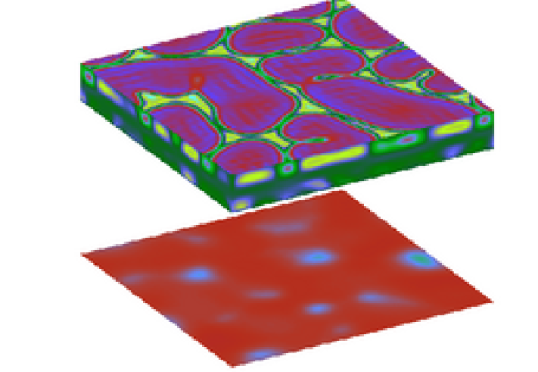
Figure 1: Relative distribution of vertical component of magnetic field ( near the top and bottom) and vertical component of momentum (sides), for the case $Q=100$ at $t=29.58$.

The bottom field is relatively weak and much more uniform, the most prominent structures being rising convergent plumes (diameter $\simeq 0.9$) with slightly enhanced values of $B_{z}$. Distinct upflow and downflow regions can be seen in the upper layer. In the central, stably stratified layer where $|\rho u_{z}|$ is small, $B_{z}$is almost uniform . The lower convection zone, in contrast to the upper layer, has fewer and less ordered convection cells, and there is little correlation with the field in the upper convection layer.

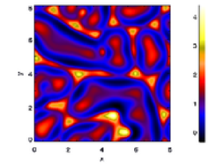
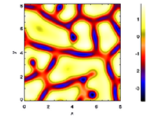
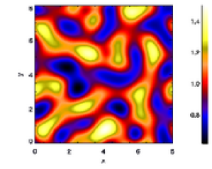
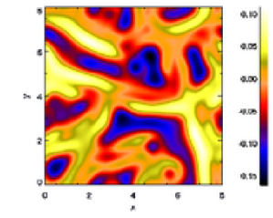
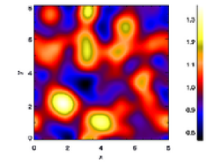
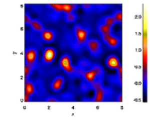
Figure 2: From top to bottom: vertical component of magnetic field (left) and vertical component of momentum (right) in the horizontal plane at $z=0.75,1.5,2.25$; for $Q=100$ and $t=29.58$.

To explore the change in flows in more detail we consider Figure 2 that shows horizontal slices of $B_{z}$ and $\rho u_{z}$ at the middle of each of the zones. At $z=0.75$, regions of high $B_{z}$ corresponds to vertical motion, and from the colourbar range on the $\rho u_{z}$ plot we see that downflows are stronger, consistent with previous studies of compressible magnetoconvection [12]. Regions of weakest $B_{z}$ matches to where $|\rho u_{z}|\sim 0$ so any motion is in the horizontal plane. This is again consistent with previous investigations, which showed that magnetic flux is swept by convection into converging regions within which the field is nearly parallel to the fluid motion [11]. We also note that in the $\rho u_{z}$ plots, there is little variation within the upflow cells.

In the convectively stable region, at $z=1.5$, there is a much smaller variation $B_{z}$ and $\rho u_{z}$ than in the upper convection zones. The pattern of motion is very weakly correlated with that at at $z=0.75$ for $B_{z}$ with rolls still dominant but of larger widths ($\sim 1$ unit). The mid-layer $\rho u_{z}$ is typically anti-correlated to the upper layer; for example the downflow region in the lower half of the plot corresponds to upflow at $z=0.75$, although the former is thinner in extent. Comparing the plots we can see that vertical field and motion at $z=0.5$ are almost unrelated. It is important to note that no convection can occur in the middle of the box because of our choice of polytropic index; so any motion must be due to overshooting plumes from either convection zone, and it would seem that the magnetic field pattern is due almost entirely to the vigorous convection in the unstable layers.

In the lower convection zone, at $z=2.25$, the contrast in $B_{z}$ is similar to that in the central region but the pattern is more cellular. Interestingly, although this layer is convectively unstable, $B_{z}$ does not correlate well to $\rho u_{z}$, unlike in the top layer. The distribution of $\rho u_{z}$ is almost uniform with small cells (diameter $\sim 0.5$ units) of strong upwards motion and their positions appear unrelated. These slice plots show distinct changes in $B_{z}$ across the layers, suggesting that for a weak field, its associated structure can not be easily communicated across boundaries, from this perspective the three layers appear independent. However, the boundary conditions on the interface allow overshooting, which is another form of communication across boundaries, and is best illustrated by considering the variation of $|\rho u_{z}|$ with $z$.

Fig. 5 shows snapshots of$\langle|\rho u_{z}|\rangle\>$and $\langle B^{2}\rangle\>$as a function of $z$ for the $Q=100$ case, where angle brackets denote horizontal averages. It is possible that such snapshots can be misleading as they can be contaminated by acoustic and gravity modes. However, we have verified by looking at other snapshots that the distributions of the two quantities shown are typical in the statistically steady state. As expected vertical motion dominates in the two convectively unstable zones due to convection, but the solid lines extend from both unstable zones into the middle so there is non-zero vertical motion throughout the stable region which indicate overshooting. The motion in the upper convection zone is more vigorous and the solid curve extends into the mid-layer more than that from the lower convection zone, which suggests more overshooting from the upper layer into the middle. This is indeed consistent with the slice plots (Figure 2); but as we will show later, the correspondence is not universal. In the statistically steady state the top also contains most of the magnetic energy. The typical value of $\langle B^{2}\rangle\>$in the middle is $\sim 0.37$ times the maximum (in the upper layer) so some of the perturbation to magnetic energy ‘overflows’ into the middle. Although there is more motion in the lower zone than the middle there is not much field amplification, and from this together with the slice plots above we conclude that stronger motions are required to increase $\langle B^{2}\rangle\>$at the bottom, as seems very reasonable given the greater density there.

Figure 3: Relative distribution of vertical component of magnetic field (near the top and bottom) and vertical momentum density (sides), for the case $Q=500$ at $t=37.12$.

Having discussed the weak field, $Q=100$ case, we now move to examine the effect of increasing the Chandrasekhar number to $Q=500$. As we have shown for the $Q=100$ case, the motion is largely confined to the top and bottom layers shown in Figure 3. Furthermore, for this $Q=500$ case, near the top we notice hexagonal-type cells of size $\sim 1.6-1.8$ dominate, the stronger field has reduced horizontal scales because particle motion is more confined along field lines. The sides of the box also show that the convection cells in the upper layer are less prominent than for $Q=100$.

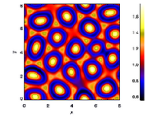
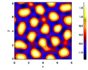
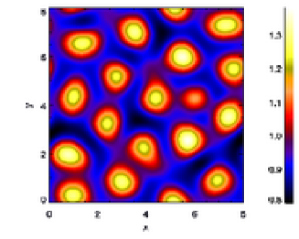
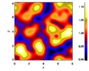
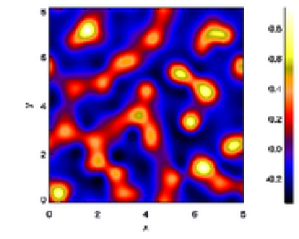
Figure 4: From top to bottom: vertical component of magnetic field (left) and vertical component of momentum (right) in the horizontal plane at $z=0.75,1.5,2.25$; for $Q=500$ and $t=37.12$.

The variation with $z$ for the $Q=500$ case is shown more clearly in Fig. 4. At $z=0.75$, $B_{z}$ is concentrated in circular and triangular cells, corresponding to upflow and downflow regions in the $\rho u_{z}$ plot. These regions of concentrated vertical flux are separated by rings with low $B_{z}$, and correspond to regions of low $|\rho u_{z}|$. At this depth there is strong correlation between field and motion; a behaviour that is similar to $Q=100$ and is again consistent with the general picture of one-layer magnetoconvection. In the stable region, at $z=1.5$, the associated disturbance to the stronger field has been effectively mirrored or transported well into the mid-layer. A possible consequence of such magnetic ‘connection’ between these two layers is that field lines may act as channels and guide particles (not possible for weak fields) from one region into another. A typical convection cell would require some horizontal motion but if this is opposed by a strong vertical field then particles are more likely to continue in the vertical direction. However, we must also note that increasing field strength is to reduce motion, as discussed later, so in terms of overshooting there is a competition between the two factors.

Fig. 4 shows the middle layer ($z=1.5$) has generally lower values of $B_{z}$ and around half as much contrast than at $z=0.75$ because motion is less vigorous and $\rho u_{z}$ at this depth is typically an order of magnitude smaller than at $z=0.75$. The figure shows no correlation between $\rho u_{z}$ and $B_{z}$ for the mid-layer, as with $Q=100$. However, in contrast to the weak field case where there is some similarity between $\rho u_{z}$ at $z=0.75,1.5$; here the hexagonal structure in the upper layer is entirely absent in the middle. Despite the strong similarity in $B_{z}$, information about vertical motion is not transported from the top to the middle. In fact, comparing $\rho u_{z}$ at $z=1.5,2.25$ show some correspondence (see, for example, the roll [in red] near the top left of the two plots). This suggests the increased field may have reduced overshooting from top and increased it from the bottom. We conclude from Fig. 4 that, since there is no requirement that $B_{z}$ and $\rho u_{z}$ to be related in a convectively stable region, the middle may echo either of the structures above or below.

Figure 5: Horizontal average of modulus of vertical momentum density (solid) and magnetic energy (solid line), as a function of depth, for $Q=100$ at $t=29.58$.

Figure 6: Horizontal average of modulus of vertical momentum (solid line) and magnetic energy divided by F (dashed line), as a function of depth, for $Q=500$ at $t=37.12$.

In order to test whether the effect of increasing the Chandrasekhar number is to reduce overshooting from the top and increase it from the bottom, we examine once again, the modulus of the vertical component of momentum density shown in Fig. 6 to compare the three regions. In conjunction with Fig. 5 ($Q=100$), we see that $\langle|\rho u_{z}|\rangle_{Q=100}>\langle|\rho u_{z}|\rangle_{Q=500}$ so increased field has generally suppressed convection. Although the plot for $Q=500$ is qualitatively very similar to that for $Q=100$ the decrease in $max(\langle|\rho u_{z}|\rangle)$ from $Q=100$ to $Q=500$ is $1.18\to 0.70$ in the upper layer and $0.29\to 0.21$ in the bottom layer and thus activity in the top layer is more strongly suppressed. This implies that the extent of overshooting from the bottom relative to that from the top has increased with field strength. Although the top has more vigorous motion, for overshooting we must consider also the direction of motion, and we will return to this when we consider $\langle\rho u_{z}\rangle\>$later. Fig. 6 shows that the variation of $\langle B^{2}\rangle\>$, in comparison to the weak field case, is smaller but that the variation with $z$ is similar. The typical value at the middle is $\sim 0.70$ times the maximum, which shows that stronger fields can increase the amount of magnetic energy pumped downwards, thereby transporting the structure and hence providing more connection. However, since the viogour of motion is suppressed (compared to $Q=100$) there is no increased overshooting from the top.

Figure 7: Relative distribution of vertical component of magnetic field (near the top and bottom) and vertical component of momentum (sides), for the case $Q=1000$ at $t=53.60$.

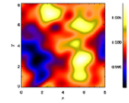
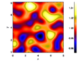
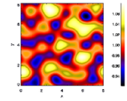
Figure 8: From top to bottom: vertical component of magnetic field in the horizontal plane at $z=0.75,1.5,2.25$; for $Q=1000$ and $t=53.60$.

We now move to discuss the $Q=1000$ case for which Fig. 7 shows an almost inverted distribution of structure and activity compared with that for $Q=100$ and $Q=500$. The bottom has magnetic structure with a horizontal scale comparable to that for the top of the $Q=500$ case, although the distribution is less ordered. Convection is predominantly in the bottom layer with typical size $\sim 2.2$ units. The strong applied field has caused the top to be almost featureless with an almost uniform $B_{z}$ and little vertical motion. The slice plots shown in Fig. 8 confirm this effect. This figure shows that the form of $B_{z}$ at $z=0.75$ is different to that at $z=1.5,2.25$ but the latter two plots are similar; the disturbance to $B_{z}$ is now transported from the bottom upwards, in contrast to the case $Q=500$. Although the plots show rich structure, note that the contrast in $B_{z}$ is only $\sim 0.01,0.05,0.12$ units for $z=0.75,1.5,2.25$ respectively, and these are all smaller than for previous cases, so the field is almost unperturbed and remains mostly vertical. However, as for previous cases we found the strongest flow-field correlation for the layer with most magnetic disturbance, which is the bottom layer for $Q=1000$. This continues the trend from $Q=100\to 500$, that overshooting from the bottom relative to the top has increased, and is further supported by Fig. 9 that show vertical motion almost completely suppressed for $z<1.7$ but $\langle|\rho u_{z}|\rangle$ is still comparable to previous cases in the lower convection zone. Since the top is suppressed, overshooting from the bottom dominates; in fact $\langle|\rho u_{z}|\rangle$ for $z>2$ is qualitatively similar to the reverse of the curve in the top layer in $Q=100$ and $Q=500$. A strong field resists deformation so there is only a 1% perturbation to $\langle B^{2}\rangle\>$. As before, the most vigorous region (bottom layer here) contains most magnetic energy but unlike previous cases the middle has a significant portion of magnetic energy. These observations are again different from that for $Q=100,500$. We have also done calculations for $Q=1500$; these show the same effect as for $Q=1000$ but to a greater degree, and for $Q=750$, which show features intermediate between the $Q=500$ and $Q=1000$ cases.

Figure 9: Horizontal average of modulus of vertical momentum (solid) and magnetic energy divided by F (dashed line), as a function of depth, for $Q=1000$ at $t=53.60$.

4 Conclusions

In this letter we have examined three-layer magnetoconvection and we have focused on the effect of varying the strength of the magnetic field via varying the Chandrasekhar number $Q$. For weak imposed magnetic field and for our parameter choices convection occurs in both the top and bottom layers. For such fields the magnetic field behaves passively and is easily swept into the intracellular regions. As we increased the strength of the magnetic field we showed at the magnetic field forces substantial changes onto the flow. We showed that for modest strength magnetic field, e.g. for the $Q=500$ case, the magnetic field forces a fairly regular convection pattern in the upper layer. However, we showed that if the magnetic field becomes too strong, as for example in the $Q=1000$ case motion in the upper convection zone is almost completely suppressed.

This preliminary work has provided the first steps towards understanding the effects of imposed magnetic fields on a stellar atmosphere with multiple unstable regions. Although the geometry is somewhat idealised, the results do show that the efficiency of overshooting and the way in which the unstable layers can communicate with each other through a stable region can be significantly affected by a magnetic field permeating all three layers. Further work at higher Rayleigh numbers is undoubtedly required to show whether the behaviour found persists in turbulent flows.

References

- [1] M. Schwarzschild, Structure and Evolution of Stars, Dover, New York, NY, 1965.
- [2] J. D. Landstreet, Astron. Astrophys. 338 (1998) 1041.
- [3] J. Silaj, A. Townsend, F. Kupka, J. Landstreet, A. Sigut, EAS Pub. Series, 17 (2005) 345.
- [4] J. Toomre, J.-P. Zahn, J. Latour, E. A. Spiegel, Astrophys. J. 207 (1976) 545.
- [5] H. J. Muthsam, W. Gob, F. Kupka, New Astronomy 4 (1999) 405.
- [6] J. Latour, E. A. Spiegel, J. Toomre, J.-P. Zahn, Astrophys. J. 207 (1976) 233.
- [7] J. Latour, J. Toomre, J.-P. Zahn, Astrophys. J. 248 (1981) 1081.
- [8] L. J. Silvers, M. R. E. Proctor, Mon. Not. R. Astron. Soc. (2007) submitted
- [9] G. Vauclair, S. Vauclair, G. Michaud, Astrophys. J. 223 (1978) 920.
- [10] G. W. Preston, Ann. Rev. Astron. Astrophys. 12 (1974) 257.
- [11] N. O. Weiss, Proc. Roy. Soc. London A. 293 (1966) 316.
- [12] N. E. Hurlburt, J. Toomre, Astrophys. J. 327 (1988) 920.
- [13] P. C. Matthews, M. R. E. Proctor, N. O. Weiss, J. Fluid Mech. 305 (1995) 281.
- [14] M. R. E. Proctor. Magnetoconvection. Invited review in: Fluid dynamics and dynamos in astrophysics and geophysics, ed. Soward, Jones, Hughes and Weiss, CRC Press, (2005) 235. tobias
- [15] S. M. Tobias, N. H. Brummell, T. L. Clune, J. Toomre, Astrophys. J. Lett. 502 (1998) 177.
- [16] S. M. Tobias, N. H. Brummell, T. L. Clune, J. Toomre, Astrophs. J. 549 (2001) 1183.
- [17] S. Vauclair, G. Vauclair, Ann. Rev. Astron. Astrophys. 20 (1982) 37.
- [18] G. Michaud, Astrophys. J. 160 (1970) 641.
- [19] E. F. Borra, J. D. Landstreet, Astrophys. J. Suppl. 42 (1980) 421.
- [20] N. E. Hurlburt, J. Toomre, J. M. Massaguer, J.-P. Zahn, Astrophys. J. 421 (1994) 245.