Shear viscosity in late time of hydrodynamic evolution in AdS/CFT duality

Abstract

We investigate the shear viscosity $\eta$ and the entropy density $s$ of strongly coupled $\mathcal{N}=4$ super Yang-Mills (SYM) plasma in late time of hydrodynamic evolution with AdS/CFT duality and Bjorken scaling. We use correlation function method proposed by Kovtun, Son and Starinets. We obtain the metric $g_{\mu\nu}$ in a proper time dependent $AdS_{5}$ space through holographic renormalization, whose boundary condition is given by energy-momentum tensor of the plasma in 2+1 dimension with transverse expansion or radial flow. With the metric we compute $\eta$ and $s$ of fluids in 1+1 and 2+1 dimension without and with radial flow. We find the ratio $\eta/s=1/(4\pi)$ in 1+1 dimension consistent with the Kovtun-Son-Starinets bound if next-to-leading terms in proper time are included in the equation of motion for metric perturbations. For 2+1 dimension the result is unchanged in the leading order of transverse rapidity.

I Introduction

Quantum chromodynamics (QCD) tells us that quarks and gluons are confined inside hadrons in vacuum or ground state. No free quarks and gluons are detected in any hadronic collisions. Finite temperature theory of QCD predicts that the deconfinement of quarks and gluons can be reached at high temperatures and densities and a new state of matter, the quark gluon plasma (QGP), can be created (Lee:1974ma, ). According to lattice QCD calculations the confinement-deconfinement phase transition takes place at temperature of about 170 MeV in three flavor case (Karsch:2000ps, ). In early 1970s Lee and Greiner and his collaborators proposed that the deconfinement could be realized by smashing two heavy ions together at ultrarelativistic energies (Hofmann:1974, ). This is the only way of generating QGP in laboratories. The minimum energy density for deconfinement to take place is about an order of magnitude higher than normal nuclear matter density. The current energy frontier of heavy ion collisions is the Relativistic Heavy Ion Collider (RHIC) at Brookhaven National Laboratory (BNL), which has been running since the summer of 2000. A lot of evidences imply that the QGP at RHIC is near perfect fluid (strongly coupled QGP or sQGP), which is contrary to the conventional concept of QGP as a weakly interacting gas of quarks and gluons, see e.g. Shuryak:2004cy ; gyulassy:2005 .

While perturbation can be used to deal with weak coupling problems, there are a lot of difficulties in describing a strongly coupled system due to its non-linear feature and failure of perturbative methods. In recent years a promising method to deal with strong coupling problems in gauge theory is through string/gauge duality or precisely AdS/CFT duality, where AdS and CFT are abbreviations for anti-de Sitter space and conformal field theory respectively. The duality was first proposed by Maldacena and many others (Maldacena:1997re, ; Gubser:1998bc, ; Witten:1998zw, ), where a strongly coupled conformal gauge field theory corresponds to weekly coupled closed strings at ’t Hooft limit. So properties of a weekly coupled string can provide information for strongly coupled gauge theory.

Policastro, Son and Starinets first used AdS/CFT duality to calculate transport coefficients of strongly coupled dense matter (Policastro:2001yc, ). Kovtun, and Son and Starinets derived a lower bound (called KSS bound) for the ratio of shear viscosity to entropy density, $\eta/s\gtrsim 1/(4\pi)$, consistent to the RHIC data Kovtun:2004de . These works open an avenue to study properties of strongly coupled matter followed by a lot of developments in hydrodynamic properties of sQGP Buchel:2003tz ; Maeda:2006by ; Natsuume:2007ty ; Baier:2007ix . Recently the jet quenching effect has been investigated with AdS/CFT techniques Liu:2006ug ; Herzog:2006gh ; Gubser:2006bz . The sceening length of the heavy quark potential can also be described from the AdS/CFT duality Liu:2006nn ; Peeters:2006iu ; Hou:2007uk ; Li:2008py , which is closely related to the $J/\psi$ suppression in hot medium.

The KSS bound is valid for any conformal fluids. Altough it is debatable that the sQGP is a conformal fluid, the ratio $\eta/s$ is fixed to be the KSS bound in all periods of the sQGP evolution in some hydrodynamic simulations (Song:2007ux, ; Chaudhuri:2008sj, ). However the sQGP formed in ultra-relativistic heavy ion collisions has particular geometric configurations such as boost invariance (Bjorken:1982qr, ) etc.. Janik and Peschanski first considered a proper time dependent $AdS_{5}$ metric with boost invariance through holographic renormalization in late time of fluid evolution Janik:2005zt ; Janik:2006ft ; Benincasa:2007tp . The method has been extended to sQGP with shear viscosity (Nakamura:2006ih, ; Sin:2006pv, ), where the shear viscosity appears in energy-momentum tensor in CFT and finally enter in the $AdS_{5}$ metric. The early time behavior of sQGP has also been addressed following similar method and can then join the late time one to provide a global picture for time evolution in heavy ion collision Kovchegov:2007pq ; Albacete:2008vs . The exact solution to the gravity dual of 1+1 dimensional sQGP with Bjorken scaling has been found by Kajantie, Louko and Tahkokallio, which is helpful to understand what happens in 1+4 dimension in the real world Kajantie:2007bn . The proper time dependent $AdS_{5}$ metric without shear viscosity does not necessarily mean that the ${\cal N}=4$ super Yang-Mills (SYM) plasma is non-viscous, noting that the shear viscosity with AdS/CFT duality is obtained by a D3 black AdS metric in Ref. (Son:2002sd, ; Son:2007vk, ). If we treat the proper time dependent $AdS_{5}$ metric without viscosity as an extension of standard AdS metric we can build up a connection between the sQGP as an ideal fluid to the SYM plasma, then the ratio $\eta/s$ may not be zero.

In this paper, we investigate the 2+1-dimensional expansion (also including 1+1-dimensional expansion) of the sQGP in late time and obtain the proper time dependent $AdS_{5}$ metric through holographic renormalization. The metric dual to the sQGP fluid can be obtained by solving the Einstein equation with the stress tensor of sQGP as boundary value of the metric if transverse expansion is small and can be treated as a perturbation. The metric has off-diagonal elements proportional to transverse rapidity. We compute with the metric the shear viscosity in 1+1 and 2+1 dimension through Kubo formula with AdS/CFT duality. In 1+1 dimension with transverse expansion turned off, the shear viscosity is found to be vanishing if only the leading terms in proper time are considered in the Einstein equation or the equation of motion for perturbations to the metric. Only including the next-to-leading terms can one get the ratio $\eta/s=1/(4\pi)$, indicating the shear viscosity is a higher order effect in late time behavior. In 2+1 dimension the result is unchanged in the leading order of transverse rapidity.

The structure of the paper is as follows. In Sec. II, we obtain the proper time dependent $AdS_{5}$ metric corresponding to the sQGP in 2+1 dimension. In Sec. III we derive the effective action for perturbations in the AdS metric. We compute the ratio $\eta/s$ in Sec. IV.1 and IV.2 for 1+1 and 2+1 dimensional cases respectively. We make summary and conclusions in Sec. V. In the paper we take the signature $(-,+,+,+,+)$ for the metric.

II 2+1 hydrodynamics with proper time dependent $AdS_{5}$ metric

II.1 2+1 hydrodynamics for ideal fluids

In order to describe the hydrodynamic evolution of an ultrarelativistic system with transverse expansion, e.g. in heavy ion collisions, we use cylindrical coordinates,

$$x^{\mu} = (\tau,y,r,\theta),$$ (1)

where $y$ is the rapidity, $\tau$ the transverse proper time, $r$ the radius in transverse plane, and $\theta$ the azimuthal angle around longitudinal direction. Note that the full proper time $\tau_{f}$ is related to $\tau$ by $\tau_{f}^{2}=\tau^{2}-r^{2}$. Hereafter the proper time means the transverse one if not explicitly stated. The line element is given by

$$ds^{2}=-d\tau^{2}+\tau^{2}dy^{2}+dr^{2}+r^{2}d\theta^{2},$$ (2)

which gives the metric $\widetilde{g}_{\mu\nu}^{(0)}=\mathrm{diag}(-1,\tau^{2},1,r^{2})$. The velocity four-vector can be parametrized as

$$u^{\mu} = \frac{dX^{\mu}}{d\tau_{f}}=\frac{1}{\sqrt{1-R^{2}(\tau,r)/\tau^{2}}}\left[1,0,\frac{R(\tau,r)}{\tau},0\right]$$ (3)

$$\equiv \left[\cosh\alpha(\tau,r),0,\sinh\alpha(\tau,r),0\right],$$

where $R$ is a function of $(\tau,r)$ and $\alpha$ is the radial rapidity in transverse direction. The radial velocity is defined by $u_{r}\equiv\sinh\alpha$. One can verify that the velocity satisfies $u^{\mu}u_{\mu}=-1$.

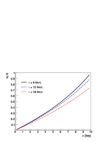
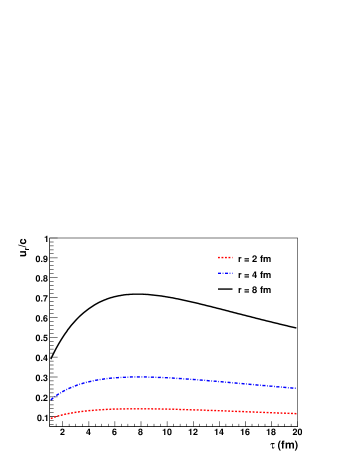
Figure 1: The radial velocity $u_{r}=\sinh\alpha$ as functions of $r$ and $\tau$.

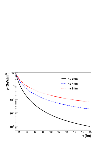
Figure 2: The radial velocity $u_{r}=\sinh\alpha$ as functions of $r$ and $\tau$.

For ideal fluid with the equation of state $\rho=3P$ where $\rho$ and $P$ are energy density and pressure respectively, the energy-momentum tensor is

$$T_{\mu\nu} = \left(\rho+P\right)u_{\mu}u_{\mu}+P\widetilde{g}_{\mu\nu}^{(0)}(x)$$ (8)

$$= \left(\begin{array}[]{cccc}-\frac{\rho}{3}+\frac{4}{3}\rho\cosh^{2}\alpha&0&-\frac{4}{3}\rho\sinh\alpha\cosh\alpha&0\\ 0&\frac{\rho}{3}\tau^{2}&0&0\\ -\frac{4}{3}\rho\sinh\alpha\cosh\alpha&0&\frac{\rho}{3}+\frac{4}{3}\rho\sinh^{2}\alpha&0\\ 0&0&0&\frac{\rho}{3}r^{2}\end{array}\right).$$

One can verify that $T_{\mu\nu}$ satisfies conformal invariance $T_{\mu}^{\mu}=0$. The energy-momentum conservation equations read

$$\nabla_{\mu}T^{\mu\nu}\equiv\partial_{\mu}T^{\mu\nu}+\Gamma_{\mu\sigma}^{\mu}T^{\sigma\nu}+\Gamma_{\mu\sigma}^{\nu}T^{\mu\sigma}=0,$$ (9)

where $\Gamma_{\mu\sigma}^{\mu}$ are Christoffel symbols for the metric in (2). The above equations lead to

$$\partial_{\tau}\ln\rho = -\frac{2}{\tau}\frac{2\cosh^{2}\alpha}{2\cosh^{2}\alpha+1}\left(1+\frac{R}{\tau}+\partial_{\tau}R\right),$$

$$\partial_{\tau}\ln R = \frac{1}{\tau}\frac{R/\tau+2+2(1-\partial_{r}R)\cosh^{2}\alpha}{2\cosh^{2}\alpha+1}.$$ (10)

Given the initial condition $R(\tau_{0},r)=\xi\tau_{0}r$ where $\xi$ is set to 0.05 $\mathrm{fm}^{-1}$, Eq. (10) can be solved numerically whose results are shown in Fig. (1)(2) and are comparable with those in Ref. (Kolb:2003dz, ). The results show that the radial velocity is linearly proportional to the radial distance, i.e. $u_{r}\sim\xi r$, where $\xi$ is a small number. One can see in the figure that $u_{r}$ rises sharply in a very short early time and gradually falls with increasing $\tau$. If the expansion in transverse direction is negligible compared to that in longitudinal direction the energy density damps in the same way as in the case of 1+1 dimension, i.e. $\rho\sim\tau^{-4/3}$.

II.2 General setup of holographic model for 2+1 hydrodynamics

In this section we briefly introduce the general idea of the holographic model for relativistic hydrodynamics. The metric in $AdS$ space can in general be written as (fefferman1985, ),

$$ds^{2} = g_{MN}dX^{M}dX^{N}=\frac{1}{z^{2}}\left[\widetilde{g}_{\mu\nu}(x,z)dx^{\mu}dx^{\nu}+dz^{2}\right],$$ (11)

where $X^{M}=(x^{\mu},z)$ and $\widetilde{g}_{\mu\nu}(x,z)$ is the metric tensor in the 4-dimensional space (1) and generally depends on $z$. Normally one assumes the following form of $\widetilde{g}_{\mu\nu}(x,z)$,

$$\widetilde{g}_{\mu\nu}(x,z)dx^{\mu}dx^{\nu}=-Ad\tau^{2}+B\tau^{2}dy^{2}+C\left(dr^{2}+r^{2}d\theta^{2}\right)+2Dd\tau dr,$$ (12)

where we have introduced the off-diagonal term proportional to $d\tau dr$ to account for transverse expansion or radial flow implied by energy-momentum tensor in (8). Note that the off-diagonal term related to transverse expansion is absent in the metric (2). One can write the coefficients $A$, $B$, $C$ and $D$ in exponential forms,

$$A=e^{w},\;B=e^{b},\;C=e^{c},\;D=e^{d}.$$ (13)

In general these coefficients are functions of $x$ and $z$. A standard way of holographic renormalization (Karch:2005ms, ; Skenderis:2002wp, ) is to expand the metric $\widetilde{g}_{\mu\nu}(x,z)$ or these coefficients in the fifth coordinate $z$,

$$\widetilde{g}_{\mu\nu}(x,z)=\sum_{n=0}z^{2n}\widetilde{g}_{\mu\nu}^{(2n)}(x),$$ (14)

where $\widetilde{g}_{\mu\nu}^{(0)}(x)$ is just the metric (2) in 4-dimensional space. The second order term $\widetilde{g}_{\mu\nu}^{(2)}(x)$ can be proved to be vanishing. The fourth order term $\widetilde{g}_{\mu\nu}^{(4)}(x)$ is given by the energy-momentum tensor,

$$\widetilde{g}_{\mu\nu}^{(4)}(x)\propto\left\langle T_{\mu\nu}\right\rangle,$$ (15)

where we set factor $\frac{N^{2}}{2\pi^{2}}=1$ ($N$ is the number of colors) and we will finally restore it. Given by these boundary conditions one can solve the $AdS$ metric (11) from the Einstein equation with the cosmological constant $\Lambda=-6$ which we will discuss about in Sec. (III),

$$R_{MN}-\frac{1}{2}g_{MN}R+6g_{MN}=0,$$ (16)

where $R_{MN}$ and $R$ are the curvature tensor and scalar in $AdS$ space with the metric $g_{MN}$ given in (11).

II.3 Holographic model in late time

The introduction of the $r$ dependence of the metric (39) makes solving the Einstein equation a formidable task even with the method of Janik and Peschanski (Janik:2005zt, ; Nakamura:2006ih, ; Sin:2006pv, ). So the simplification is necessary. In this section we consider a simplified problem with perturbation in transverse direction based on the Janik-Peschanski method.

Supposing $\alpha$ is small in Eq. (8) we can make an expansion of $T_{\mu\nu}$ in $\alpha$,

$$T_{\mu\nu} = \left(\begin{array}[]{cccc}\rho&0&0&0\\ 0&\tau^{2}\frac{1}{3}\rho&0&0\\ 0&0&\frac{1}{3}\rho&0\\ 0&0&0&r^{2}\frac{1}{3}\rho\end{array}\right)+\alpha\left(\begin{array}[]{cccc}0&0&-\frac{4}{3}\rho&0\\ 0&0&0&0\\ -\frac{4}{3}\rho&0&0&0\\ 0&0&0&0\end{array}\right)$$ (30)

$$+\alpha^{2}\left(\begin{array}[]{cccc}\frac{4}{3}\rho&0&0&0\\ 0&0&0&0\\ 0&0&\frac{4}{3}\rho&0\\ 0&0&0&0\end{array}\right)+O\left(\alpha^{3}\right).$$

In this expansion, we see that off-diagonal elements are proportional to odd power of $\alpha$, while modifications of diagonal elements are proportional to even power of $\alpha$. In leading order the transverse velocity vanishes and we reproduce the results in Ref. (Janik:2005zt, ; Nakamura:2006ih, ). In next-to-leading order $O(\alpha)$ the transverse velocity does not vanish while the energy density and pressure do not change, whose modifications are in $O(\alpha^{2})$ or higher.

If we assume that there is no linear terms of $\alpha$ in diagonal components of the AdS metric $g_{MN}$, we get the following result by solving the Einstein equation (16),

$$g_{MN}=\frac{1}{z^{2}}\left(\begin{array}[]{ccccc}-\frac{(1-a)^{2}}{1+a}&0&\frac{4}{3}\alpha\frac{(1-a)^{2}}{1+a}&0&0\\ 0&\tau^{2}(1+a)&0&0&0\\ \frac{4}{3}\alpha\frac{(1-a)^{2}}{1+a}&0&1+a&0&0\\ 0&0&0&r^{2}(1+a)&0\\ 0&0&0&0&1\end{array}\right),$$ (31)

with $a=\frac{\rho_{0}z^{4}}{3\tau^{4/3}}$ and $\rho_{0}$ is a constant energy density.

In the case without off-diagonal components in the metric (31), i.e. $\alpha=0$, the line element in central rapidity region (not for non-central rapidity region) has the form,

$$ds^{2}=-\frac{(1-z^{4}/z_{H}^{4})^{2}}{1+z^{4}/z_{H}^{4}}\frac{d\tau^{2}}{z^{2}}+\frac{1+z^{4}/z_{H}^{4}}{z^{2}}[\tau^{2}dy^{2}+dr^{2}+r^{2}d\theta^{2}]+\frac{dz^{2}}{z^{2}},$$ (32)

where the black hole locates at

$$z_{H}=\left(\frac{\rho_{0}}{3}\right)^{-1/4}\tau^{1/3},$$ (33)

which depends on $\tau$. See Appendix (A) for the derivation of the metric (32). Changing variables,

$$z\rightarrow\widetilde{z}=\frac{z}{\sqrt{1+\frac{z^{4}}{z_{H}^{4}}}},\qquad z_{H}\rightarrow\widetilde{z}_{H}=\frac{z_{H}}{\sqrt{2}},$$ (34)

we can verify that the line element (32) is the standard one in D3 black $AdS_{5}$ space if $z_{0}$ is constant, see Sec. III,

$$ds^{2}=-\frac{1-\widetilde{z}^{4}/\widetilde{z}_{H}^{4}}{\widetilde{z}^{2}}d\tau^{2}+\frac{d\mathbf{x}^{2}}{\widetilde{z}^{2}}+\frac{1}{1-\widetilde{z}^{4}/\widetilde{z}_{H}^{4}}\frac{d\widetilde{z}^{2}}{\widetilde{z}^{2}},$$ (35)

where $d\mathbf{x}^{2}\equiv\tau^{2}dy^{2}+dr^{2}+r^{2}d\theta^{2}$ and $\widetilde{z}_{H}$ is the location of the black hole horizon, the cosmology constant for $AdS_{d+1}$ is (Skenderis:2002wp, )

$$\Lambda=-\frac{d(d-1)}{2}=-6,$$ (36)

and the Hawking temperature is determined by the behavior of the metric near the horizon,

$$T_{H}=\frac{1}{\pi\widetilde{z}_{H}}=\frac{\sqrt{2}}{\pi z_{H}}.$$ (37)

Hereafter we call the proper time dependent $AdS_{5}$ metric the $AdS^{\#}$ one in (31) with transverse expansion or in (32) without transverse expansion.

III Effective action for perturbations in $AdS$ metric

The low energy limit of type IIB string theory in $AdS_{5}\times S^{5}$ space can be approximated by a five-dimensional theory (see, e.g. Son:2007vk ) whose action is

$$I_{5D}\approx\frac{N^{2}}{8\pi^{2}R^{3}}\int d^{5}x(\mathcal{R}_{5D}-2\Lambda+\cdots),$$ (38)

where $\mathcal{R}_{5D}$ is the scalar curvature in $AdS_{5}$, $\Lambda$ the cosmological constant, and $R$ the radius of $S^{5}$. The line element in $AdS_{5}$ space without black hole is

$$ds^{2}=\frac{r^{2}}{R^{2}}(-dt^{2}+d\mathbf{x}^{2})+\frac{R^{2}}{r^{2}}dr^{2}.$$ (39)

Using the variable $z=R^{2}/r$, the above line element can be written as

$$ds^{2}=\frac{R^{2}}{z^{2}}(-dt^{2}+d\mathbf{x}^{2}+dz^{2}).$$ (40)

The line element with a black hole has the form

$$ds^{2} = \frac{R^{2}}{z^{2}}\left[-(1-z^{4}/z_{H}^{4})dt^{2}+d\mathbf{x}^{2}+\frac{1}{1-z^{4}/z_{H}^{4}}dz^{2}\right]$$ (41)

$$= \frac{\pi^{2}T^{2}R^{2}}{u}[-(1-u^{2})dt^{2}+d\mathbf{x}^{2}]+\frac{R^{2}}{4u^{2}(1-u^{2})}du^{2},$$

where $u=z^{2}/z_{H}^{2}$ and $z_{H}=1/(\pi T)$.

The AdS/CFT correspondence can be expressed by

$$Z_{4D}[J]=\left.e^{iS_{5D}[\phi]}\right|_{J(x)=\phi(x,z=0)},$$ (42)

where $Z_{4D}[J]$ is the partition function of CFT in 4-dimensional Minkowski space and $S_{5D}[\phi]$ the action in $AdS_{5}$ given by (38) for the classical bulk field $\phi(x,z)$, $J(x)$ is the source in 4-dimension taking the value of the bulk field on the boundary $z=0$ in $AdS_{5}$. The partition function $Z_{4D}[J]$ is a functional of $J(x)$,

$$Z_{4D}[J]=\int[d\varphi]\mathrm{exp}\left\{iS_{CFT}[\varphi]+i\int d^{4}xJO[\varphi]\right\},$$ (43)

where $\varphi$ denotes the CFT fields, $O[\varphi]$ is the operator coupling to $J(x)$, and $S_{CFT}[\varphi]$ is the CFT action. Following the AdS/CFT correspondence the Green functions of operators $O$ in CFT can be evaluated in terms of $S_{5D}[\phi]$ in $AdS_{5}$, for example, a two-point Green function is

$$\left\langle TO(x_{1})O(x_{2})\right\rangle_{4D}=\left.\frac{\delta^{2}S_{5D}[\phi]}{i\delta\phi(x_{1})\delta\phi(x_{2})}\right|_{J(x)=\phi(x,z=0)}.$$ (44)

We note that the stress tensor is coupled with the metric,

$$T_{\mu\nu}=-\frac{2}{\sqrt{-\widetilde{g}}}\frac{\delta S_{CFT}}{\delta\widetilde{g}_{\mu\nu}},$$ (45)

where $T_{\mu\nu}$ can be regarded as an operator in CFT and the metric $\widetilde{g}_{\mu\nu}$ in 4-dimension as its source. In order to obtain the shear viscosity $\eta$ through the Kubo formula,

$$\eta=-\lim_{\omega\rightarrow 0}\frac{1}{\omega}\mathsf{\mathrm{Im}}G_{12,12}^{R}(\omega,\mathbf{0}),$$ (46)

we need to know the Green function of $T_{12}$ at low energy limit,

$$G_{12,12}^{R}(\omega,\mathbf{k})=-i\int d^{4}xe^{ik\cdot x}\Theta(t)\left\langle[T_{12}(x),T_{12}(0)]\right\rangle.$$ (47)

To obtain $G_{12,12}^{R}(\omega,\mathbf{k})$ from the gravitational dual we should know the action $S_{5D}[g_{\mu\nu}]$ in $AdS_{5}$ as a functional of $g_{\mu\nu}$ with the boundary value $g_{\mu\nu}(z=0)\rightarrow\widetilde{g}_{\mu\nu}$. For this purpose we consider a variation in the $AdS_{5}$ metric, $g_{\mu\nu}=g_{\mu\nu}^{(0)}+h_{\mu\nu}$. We can choose for simplicity $h_{z\mu}=h_{\mu z}=0$ and that $h_{\mu\nu}$ depend on $t$, $x^{3}$ and $z$ (or $u$). The line element in (41) then becomes

$$ds^{2}=\frac{\pi^{2}T^{2}R^{2}}{u}[-(1-u^{2})dt^{2}+d\mathbf{x}^{2}]+\frac{R^{2}}{4u^{2}(1-u^{2})}du^{2}+h_{\mu\nu}dx^{\mu}dx^{\nu}.$$ (48)

We can expand the action (38) in terms of $h_{\mu\nu}$,

$$I_{5D} \approx \frac{N^{2}}{8\pi^{2}}\int d^{5}x\sqrt{-g}(\mathcal{R}_{\mu\nu}-\frac{1}{2}g_{\mu\nu}\mathcal{R}+\Lambda g_{\mu\nu})h^{\mu\nu}$$ (49)

$$= \frac{N^{2}}{8\pi^{2}}\int d^{5}x\sqrt{-g}(\mathcal{R}_{\mu\nu}^{(0)}-\frac{1}{2}g_{\mu\nu}^{(0)}\mathcal{R}_{(0)}+\Lambda g_{\mu\nu}^{(0)})h^{\mu\nu}$$

$$+\frac{N^{2}}{8\pi^{2}}\int d^{5}x\sqrt{-g}(\delta\mathcal{R}_{\mu\nu}-\frac{1}{2}h_{\mu\nu}\mathcal{R}_{(0)}-\frac{1}{2}g_{\mu\nu}^{(0)}\delta\mathcal{R}+\Lambda h_{\mu\nu})h^{\mu\nu}$$

$$= \frac{N^{2}}{8\pi^{2}}\int d^{5}x\sqrt{-g}(\delta\mathcal{R}_{\mu\nu}-\frac{1}{2}g_{\mu\nu}^{(0)}\delta\mathcal{R}+4h_{\mu\nu})h^{\mu\nu},$$

where we have used the fact that the first term of the second equality is vanishing from the Einstein equation for the unperturbed metric $g_{\mu\nu}^{(0)}$. We have also used $\mathcal{R}_{0}=-20$ and $\Lambda=-6$. Here we have chosen the $S^{5}$ radius $R=1$. We consider the components $h_{12}=h_{21}$ which can be verified to decouple from others. For the metric (48), the action (49) can be simplified as

$$I_{5D} \approx \frac{N^{2}}{8\pi^{2}}\int d^{5}x\sqrt{-g}(\delta R_{12}+4h_{12})h^{12}=\frac{N^{2}}{8\pi^{2}}\int d^{5}x\sqrt{-g}\left(-\frac{1}{2}g^{\mu\nu}\partial_{\mu}\phi\partial_{\nu}\phi+\cdots\right),$$ (50)

with $\phi=h_{2}^{1}=g^{11}h_{12}$ and $h^{12}=-g^{11}g^{22}h_{12}$. The retarded two-point Green functions of the CFT stress tensor can then be derived from the quadratic terms in $I_{5D}$ as above by using Eq. (44). The shear viscosity is then obtained through the Kubo formula (46).

IV Shear viscosity and entropy density in $AdS_{5}^{\#}$

In this section we will calculate the shear viscosity in $AdS_{5}^{\#}$ following the procedure of AdS/CFT duality presented in the previous section. Also we will compute the entropy density in $AdS_{5}^{\#}$. We consider fluid evolutions in 1+1/2+1 dimension without/with transverse expansion or radial flow.

IV.1 1+1 dimension without transverse expansion

Following Janik and Peschanski’s solution (Janik:2005zt, ) in late time, the line element in $AdS_{5}^{\#}$ in 1+1 dimension can be written as

$$ds^{2}=\frac{1}{z^{2}}\left\{-\frac{(1-a)^{2}}{1+a}d\tau^{2}+(1+a)[\tau^{2}dy^{2}+dx_{1}^{2}+dx_{2}^{2}]\right\}+\frac{dz^{2}}{z^{2}},$$ (51)

where $a=\frac{\rho_{0}z^{4}}{3\tau^{4/3}}$. Note that the derivative of $a$ is non-zero, i.e. $\partial_{\tau,z}a\neq 0$ in computing the Ricci tensor and the scalar curvature. Finally we will keep a constant $a$ while taking the limit $\tau\rightarrow\infty$ when doing power counting in $\tau$. In adopting the above measure we can verify after a lenghy but straightforward algebra that the Ricci tensor $\mathcal{R}_{\mu\nu}=-4g_{\mu\nu}$ and $\mathcal{R}_{5D}=-20$ upto higher order terms in negative powers of $\tau$. The determinant of the metric is $\sqrt{-g}=\frac{1}{z^{5}}(1-a^{2})\tau$. Taking a perturbation in the metric $g_{\mu\nu}=g_{\mu\nu}^{(0)}+h_{\mu\nu}$ with $h_{12}=h_{12}(\tau,y,z)$ and $h_{\mu\nu}=0$ for all other indices $\mu,\nu$, we obtain the quadratic terms of the effective action up to higher order contributions in negative powers of $\tau$,

$$I_{5D}\approx-\frac{N^{2}}{16\pi^{2}}\int d^{5}x\sqrt{-g}g^{\mu\nu}\partial_{\mu}\phi\partial_{\nu}\phi,$$ (52)

where $\phi\equiv h_{2}^{1}=g^{11}h_{12}$, $d^{5}x=d\tau dydx_{1}dx_{2}dz$ and $\mu=\tau,y,1,2,z$. The equation of motion for $\phi$ is then

$$\partial_{\mu}(\sqrt{-g}g^{\mu\nu}\partial_{\nu}\phi)=0.$$ (53)

We assume a factorized form for $\phi$,

$$\phi(\tau,y,z)=\phi_{0}(y,\tau)f(z)=\int\frac{d\omega dp_{3}}{(2\pi)^{2}}\exp(-i\omega\tau\cosh y+ip_{3}\tau\sinh y)\phi_{0}(\omega,p_{3})f_{p}(z)$$ (54)

where $p_{3}$ is the momentum along the third axis (we do not distinguish subscript or superscript for this mometum). Inserting the above into Eq. (53) and taking the limit $\tau\rightarrow\infty$ while keeping $v$ or $a$ constant, the leading order contribution of $O(\tau^{0})$ in Eq. (8) gives

$$0 = (1-a^{2})\frac{d^{2}f_{p}}{dz^{2}}+f_{p}\frac{(1+a)^{2}}{1-a}\omega^{2}\cosh^{2}y-f_{p}(1-a)(-\omega\sinh y+p_{3}\cosh y)^{2}.$$ (55)

We consider the central rapidity $y=0$ and static limit $p_{3}=0$, the above equation becomes

$$\frac{d^{2}f_{p}}{dz^{2}}+\frac{(1+a)}{(1-a)^{2}}\omega^{2}f_{p}=0.$$ (56)

The reason for choosing central rapidity is that the metric (51) can only be treated as an extension of the standard AdS one at central rapidity, see Appendix A. Considering the solution near the horizon at $a_{H}=1$ and changing variables,

$$z \rightarrow z^{\prime}=\left(\frac{\rho_{0}}{3}\right)^{1/4}\tau^{-1/3}z,$$

$$\omega^{\prime} \rightarrow \frac{1}{2\sqrt{2}}\left(\frac{\rho_{0}}{3}\right)^{-1/4}\tau^{1/3}\omega,$$ (57)

Eq. (56) can be rewritten

$$\frac{d^{2}f_{p}}{d{z^{\prime}}^{2}}+\frac{1}{(1-z^{\prime})^{2}}{\omega^{\prime}}^{2}f_{p}=0.$$ (58)

The solution to Eq. (58) can be found,

$$f_{p}(z)=(1-z^{\prime})^{1/2(1\pm\sqrt{1-4{\omega^{\prime}}^{2}})}\approx(1-z^{\prime})^{1/2\pm i\omega^{\prime}},$$ (59)

where we have approximated $\sqrt{1-4{\omega^{\prime}}^{2}}\approx i2\omega^{\prime}$ at the limit $\tau\rightarrow\infty$, since $\omega^{\prime}\sim\tau^{1/3}\gg 1$. Using the incoming wave solution corresponding to the positive sign in (59) and substituting it back into the action (52), the boundary term at $z=z_{H}$ or the black hole horizon at $a_{H}=1$, the retarded Green function $G_{12,12}^{R}(\omega)$ at the static limt can be obtained, which is vanishing due to the presence of the real part $\frac{1}{2}$ in the exponent of the solution (59). This can be seen from the fact that there is a factor $(1-z^{\prime})$ which is zero at the boundary, see Eq. (79) in Appendix (B). Therefore we have shown that the shear viscosity is absent from the scaling solution in 1+1 dimension in the leading order.

Picking up the next-to-leading order contribution of $O(1/\tau^{1/3})$ in Eq. (53), Eq. (56) becomes

$$\frac{d^{2}f_{p}}{dz^{2}}-\frac{3+5a^{2}}{z(1-a^{2})}\frac{df_{p}}{dz}+\frac{(1+a)}{(1-a)^{2}}\omega^{2}f_{p}=0.$$ (60)

Changing variables as in Eq. (57), the above equation near the horizon can be rewritten in the form

$$\frac{d^{2}f_{p}}{d{z^{\prime}}^{2}}-\frac{1}{1-z^{\prime}}\frac{df_{p}}{dz^{\prime}}+\frac{1}{(1-z^{\prime})^{2}}{\omega^{\prime}}^{2}f_{p}=0,$$ (61)

whose solutions are

$$f_{\pm p}(z)=(1-z^{\prime})^{\pm i\omega^{\prime}}.$$ (62)

As derived in Eq. (80) in Appendix B, the retarded Green function at static limit is obtained,

$$G_{12,12}^{R}(\omega,0)=-2F(\omega)=-i\frac{\sqrt{2}}{3^{3/4}\times 4\pi^{2}}N^{2}\rho_{0}^{3/4}\tau^{-1}\omega.$$ (63)

The shear viscosity per unit transverse area can be obtained from the Kubo formula (46),

$$\eta=\frac{\rho_{0}^{3/4}\sqrt{N}}{6^{3/4}\sqrt{\pi}}\frac{1}{\tau}.$$ (64)

where we have recovered the factor $\rho_{0}\rightarrow\rho_{0}\left(\frac{N^{2}}{2\pi^{2}}\right)^{-1}$.

The Hawking temperature is $T=\frac{\sqrt{2}}{\pi z_{H}}$ from Eq. (37) where $z_{H}$ is the horizon of the black hole given in Eq. (33). Then the initial energy density is a constant due to $T\sim\tau^{-1/3}$,

$$T=\frac{\sqrt{2}}{\pi z_{H}}=\frac{\sqrt{2}}{\pi}\left(\frac{2\pi^{2}\rho_{0}}{3N^{2}}\right)^{1/4}\tau^{-1/3}.$$ (65)

The entropy per unit rapidity and unit transverse area is given by (Janik:2005zt, ; Sin:2006pv, ),

$$S=\left(\frac{N^{2}}{2\pi}\right)^{1/4}\left(\frac{\pi}{3}\right)^{3/4}2\sqrt{2}\rho_{0}^{3/4}=\frac{N^{2}}{2}\pi^{2}T^{3}\tau.$$ (66)

The entropy density is obtained,

$$s=\frac{S}{\tau}=\frac{1}{2}N_{c}^{2}\pi^{2}T^{3},$$ (67)

where we see that the entropy density has an asymptotic behavior $s\sim\tau^{-1}$. From Eq. (64) and (67), we get the well-known value,

$$\frac{\eta}{s}=\frac{1}{4\pi}.$$ (68)

IV.2 2+1 dimension with transverse expansion

The metric in 2+1 dimension with radial flow is given in (31), in order to calculate the shear viscosity we have to introduce a perturbation to the background metric. It is then convenient to explicitly use rectangular transverse coordinates $(x_{1},x_{2})$ instead of cylindrical ones $(r,\theta)$. The corresponding line element is

$$ds^{2}=\frac{1}{z^{2}}\left\{-\frac{(1-a)^{2}}{1+a}dt^{2}+(1+a)(dx_{3}dx_{3}+dx_{i}dx_{i})+\frac{8}{3}\alpha\frac{(1-a)^{2}}{1+a}\frac{1}{r}x_{i}dx_{i}dt+\frac{dz^{2}}{z^{2}}\right\},$$ (69)

where $r=\sqrt{x_{i}x_{i}}$ and the summation over $i=1,2$ is implied. We keep in mind that $\alpha$ is small. The metric determinant has the same form as in the 1+1 dimensional case in the leading order,

$$\sqrt{-g}=\frac{1}{z^{5}}(1-a^{2})+O(\alpha^{2}).$$ (70)

Now we consider the perturbation $h_{12}(t,x_{3},z)$ to the background metric (69). Denoting $\phi=h_{2}^{1}(t,x_{3},z)$, we find the equation of motion for $\phi$,

$$0=\delta\mathcal{R}_{2}^{1}+4\phi=-\frac{1}{2\sqrt{-g}}\partial_{\mu}(\sqrt{-g}g^{\mu\nu}\partial_{\nu}\phi).$$ (71)

It can be verified that the entangled term $\sim\alpha\phi$ appear in $O(t^{-1/3})$, while leading terms are of $O(t^{2/3})$. So the transverse part is decoupled from $\phi$ in the leading order. The shear viscosity and entropy density per unit transverse area are the same as in the 1+1 dimensional case, Eqs. (64) and (67).

We can also consider the perturbation along $x_{2}$ axis (or equivalently $x_{1}$ axis), i.e. $\phi=h_{3}^{1}(t,z,x_{2})$. To the leading order $O(\tau^{2/3})$ we find the equation of motion for $\phi$,

$$0=\delta\mathcal{R}_{3}^{1}+4\phi=-\frac{1}{2\sqrt{-g}}\partial_{\mu}(\sqrt{-g}g^{\mu\nu}\partial_{\nu}\phi)+t^{2/3}\frac{2}{3}\alpha\frac{1}{1+a}\frac{(x^{2})^{2}}{r^{3}}\partial_{t}\phi,$$ (72)

whose explicit form reads,

$$-\partial_{z}^{2}\phi+\frac{1+a}{(1-a)^{2}}\partial_{t}^{2}\phi-\frac{4}{3}\alpha\frac{1}{1+a}\frac{(x^{1})^{2}}{r^{3}}\partial_{t}\phi=0.$$ (73)

We see that the transverse part enters the equation of motion in the leading order. We assume that the solution has the factorization form $\phi(t,x_{2},z)=\phi_{0}(p)f_{p}(z)e^{-i\omega t+ip_{2}x_{2}}$, then we derive from Eq. (73) the differential equation for $f_{p}(z)$,

$$\frac{d^{2}f_{p}}{dz^{2}}-\frac{3+5a}{z(1-a^{2})}\frac{df_{p}}{dz}+\frac{1+a}{(1-a)^{2}}\omega^{2}f_{p}-\frac{i}{1+a}\frac{2\alpha}{3r}\omega f_{p}=0,$$ (74)

where we can expand the equation near the horzion $z\rightarrow z_{H}$ in Eq. (33),

$$\frac{d^{2}f_{p}}{d{z^{\prime}}^{2}}-\frac{1}{1-z^{\prime}}\frac{df_{p}}{dz^{\prime}}+\frac{1}{(1-z^{\prime})^{2}}{\omega^{\prime}}^{2}f_{p}-i\alpha\frac{2\sqrt{2}z_{H}}{3r}\omega^{\prime}f_{p}=0.$$ (75)

The solution is a linear combination of Bessel functions,

$$f_{p1} = J_{i\omega^{\prime}}\left[i^{3/2}(1-z^{\prime})z_{H}\sqrt{\frac{\alpha\omega}{3r}}\right],$$

$$f_{p2} = Y_{i\omega^{\prime}}\left[i^{3/2}(1-z^{\prime})z_{H}\sqrt{\frac{\alpha\omega}{3r}}\right].$$

Since $\alpha$ is small, we can make expansion in $\alpha$ for the solutions $f_{p1}$ and $f_{p2}$. One can verify that the solution is a linear combination of $f_{p}$ and $f_{-p}$,

$$f_{p} = (1-z^{\prime})^{i\omega^{\prime}}z_{H}^{i\omega^{\prime}}\left(\frac{\alpha\omega}{3r}\right)^{i\omega^{\prime}}\left[\frac{(-1)^{i3\omega^{\prime}/4}2^{-i\omega^{\prime}}}{\Gamma(1+i\omega^{\prime})}+\frac{i(-1)^{i3\omega^{\prime}/4}2^{-2-i\omega^{\prime}}}{(1+i\omega^{\prime})\Gamma(1+i\omega^{\prime})}(1-z^{\prime})^{2}z_{H}^{2}\frac{\alpha\omega}{3r}\right],$$

$$f_{-p} = f_{p}(i\omega^{\prime}\rightarrow-i\omega^{\prime}).$$ (76)

One sees that $f_{-p}=f_{p}^{*}$. Following Eq. (81) in Appendix B and steps in previous section, we get the same value as in the case of 1+1 dimension, i.e. $\eta/s=1/(4\pi)$.

V Summary and discussions

We derive a time dependent metric dual to sQGP fluid in 2+1 dimension with radial flow in late time by holographic renormalization. It is difficult to obtain the exact solution to the Einstein equation with this metric, especially when the metric has off-diagonal components for radial flows. If transverse expansion is small and can be treated as a perturbation, the late time asymptotic solution, the metric in (31) with off-diagonal elements, can be found by using $v=z^{4}/\tau^{4/3}$ as a scaling and expansion parameter. With this metric we calculate the ratio $\eta/s$ of shear viscosity $\eta$ to entropy density $s$ for sQGP in SYM field theory with the KSS method. As a first attempt we consider 1+1 dimension with only longitudinal flow whose metric is diagonal. If we include only the leading order terms in the equation of motion for perturbations to the metric, the shear viscosity is vanishing, consistent to the assumption that the fluid is ideal. We reproduce KSS bound $1/(4\pi)$ for $\eta/s$ if we pick up the next-to-leading order term in the equation of motion, indicating that the shear viscosity is a higher order effect. Our derivation is based on the Janik and Peschanski’s method and is valid in late time, $\tau\rightarrow\infty$. For intermidiate stage of hydrodynamic evolution the ratio is not necessarily $1/(4\pi)$ for an expanding fluid, so our result is not trivial or obvious. We further show that the ratio for fluids in 2+1 dimension in late time with transverse flow is the same as in 1+1 dimension in the leading order of transverse rapidity. We remember that the mean free path is $l_{\mathrm{mfp}}\sim 1/(n\sigma v)$, where $n\sim T^{3}$ is the particle number density, $\sigma\sim g^{2}T^{-2}$ ($g$ is the coupling constant) the typical scattering cross section and $v\sim 1$ the typical velocity. The shear viscosity can then be estimated as $\eta\sim\rho l_{\mathrm{mfp}}\sim g^{-2}T^{3}$, where $\rho$ is the energy density. In comparsion with our result in Eq. (64), we have $\eta\sim\tau^{-1}$, $T\sim\tau^{-1/3}$ and $g$ does not change with the proper time. This implies that if the coupling is as strong at the beginning as in late time of fluid expansion or hydrodynamic evolution does not influence the strength of the interaction.

In 1+1 dimension one can introduce the shear viscosity of the next-to-leading order in the stress tensor in late time solution Janik:2006ft ; Nakamura:2006ih ; Sin:2006pv . So an interesting attempt is to calculate the shear viscosity with the metric dual to the stress tensor with shear terms. We found that the correction to the shear viscosity is also of the next-to-leading order, $\eta/s=1/(4\pi)+O(\tau^{-1-s})$.

The same analysis can also be applied to hydrodynamic behaviors of sQGP in early time, which is important to understand the initial state of QGP Kovchegov:2007pq . However early time behaviors of fluids show anisotropic feature and therefore more complicated. We will reserve it for a future investigation.

Appendix A Derivation of the metric in (32)

The D3 black AdS metric can be writen as

$$ds^{2}=-\frac{(1-z^{4}/z_{0}^{4})^{2}}{1+z^{4}/z_{0}^{4}}dt^{2}+(1+z^{4}/z_{0}^{4})\frac{d\mathbf{x}^{2}}{z^{2}}+\frac{dz^{2}}{z^{2}}.$$ (77)

Changing variables to $(t,x^{3})\rightarrow(\tau,y)$ through $t=\tau\cosh y$, $x^{3}=\tau\sinh y$, the metric becomes

$$ds^{2} = (-A\cosh^{2}y+B\sinh^{2}y)d\tau^{2}+\tau^{2}(-A\sinh^{2}y+B\cosh^{2}y)dy^{2}$$ (78)

$$+2\tau(-A+B)\cosh y\sinh yd\tau dy+...$$

where $A=\frac{(1-z^{4}/z_{0}^{4})^{2}}{1+z^{4}/z_{0}^{4}}$ and $B=(1+z^{4}/z_{0}^{4})$. The metric (78) has the symmetry under $y\rightarrow-y$. In comparsion with Janik and Peschanski’s time dependence metric, there is an off-diagonal part $\sim d\tau dy$ in the metric (78). So the metric (32) is only valid in central rapidity region around $y\sim 0$.

Appendix B Evaluation of retarded Green function from solution (59)

Substituting the solutions $f_{\pm}$ in (59) and (62) back into the action (38) and keep the boundary term at $z=z_{H}$, we find

$$I_{5D} = -\frac{N^{2}}{16\pi^{2}}\int d^{4}xdz\frac{\partial}{\partial z}[\sqrt{-g}g^{zz}\phi(\tau,y,z)\partial_{z}\phi(\tau,y,z)]$$

$$= -\frac{N^{2}}{16\pi^{2}}\int d^{4}x\tau\left.\frac{1-a^{2}}{z^{3}}\phi(\tau,y,z)\partial_{z}\phi(\tau,y,z)\right|_{z=z_{H}}$$

$$= -\frac{N^{2}}{16\pi^{2}}\int d\tau dydx^{1}dx^{2}\tau\int\frac{d\omega dp_{3}d\omega^{\prime}dp_{3}^{\prime}}{(2\pi)^{4}}\exp[-i(\omega+\omega^{\prime})\tau\cosh y+i(p_{3}+p_{3}^{\prime})\tau\sinh y]$$

$$\times\phi_{0}(\omega,p_{3})\phi_{0}(\omega^{\prime},p_{3}^{\prime})\left.\frac{1-a^{2}}{z^{3}}f_{p^{\prime}}(z)\frac{df_{p}(z)}{dz}\right|_{z=z_{H}}$$

$$= -\frac{N^{2}}{16\pi^{2}}\int d(\tau\cosh y)d(\tau\sinh y)dx^{1}dx^{2}\int\frac{d\omega dp_{3}d\omega^{\prime}dp_{3}^{\prime}}{(2\pi)^{4}}$$

$$\times\exp[-i(\omega+\omega^{\prime})\tau\cosh y+i(p_{3}+p_{3}^{\prime})\tau\sinh y]\phi_{0}(\omega^{\prime},p_{3}^{\prime})\phi_{0}(\omega,p_{3})$$

$$\times\left.\frac{1-a^{2}}{z^{3}}f_{p^{\prime}}(z)\frac{df_{p}(z)}{dz}\right|_{z=z_{H}}$$

$$= -\frac{N^{2}}{16\pi^{2}}\int dx^{1}dx^{2}\int\frac{d\omega dp_{3}}{(2\pi)^{2}}\phi_{0}(-\omega,-p_{3})\phi_{0}(\omega,p_{3})\left.\frac{1-a^{2}}{z^{3}}f_{-p}(z)\frac{df_{p}(z)}{dz}\right|_{z=z_{H}}$$

$$\equiv \int\frac{d^{4}p}{(2\pi)^{4}}\phi_{0}(-\omega,-p)\phi_{0}(\omega,p)F(\omega).$$

In the fourth equality we have changed the integral variables, $d\tau dy\tau=d(\tau\cosh y)d(\tau\sinh y)$. In the last we have assumed that $\phi_{0}(\omega,p)=(2\pi)^{2}\delta(p_{1})\delta(p_{2})\phi_{0}(-\omega,-p_{3})$ and set the transverse area $L^{2}=1$. Now we evaluate $F(\omega)$. For the solutions (59), we have

$$F(\omega) \propto \lim_{z\rightarrow z_{H}}\frac{1-a^{2}}{z^{3}}f_{-p}(z)\frac{df_{p}(z)}{dz}$$ (79)

$$= \frac{8}{z_{H}^{3}}\lim_{z\rightarrow z_{H}}(1-z^{\prime})(1-z^{\prime})^{1/2-i\omega^{\prime}}\frac{d}{dz}(1-z^{\prime})^{1/2+i\omega^{\prime}}$$

$$= -\frac{8}{3}\rho_{0}\tau^{-4/3}(1/2+i\omega^{\prime})\lim_{z\rightarrow z_{H}}(1-z^{\prime})$$

$$= 0,$$

while for the solutions (62), we obtain

$$F(\omega) = -\frac{N^{2}}{16\pi^{2}}\left.\frac{1-a^{2}}{z^{3}}f_{-p}(z)\frac{df_{p}(z)}{dz}\right|_{z=z_{H}}$$ (80)

$$= i\frac{N^{2}}{16\pi^{2}}\omega^{\prime}\frac{8}{3}\rho_{0}\tau^{-4/3}\lim_{z\rightarrow z_{H}}(1-z^{\prime})(1-z^{\prime})^{-i\omega^{\prime}}(1-z^{\prime})^{i\omega^{\prime}-1}$$

$$= i\omega\frac{\sqrt{2}N^{2}}{8\pi^{2}}\left(\frac{\rho_{0}}{3}\right)^{3/4}\tau^{-1}.$$

For the solution (76), we get

$$F(\omega) = -\frac{N^{2}}{16\pi^{2}}\left.\frac{1-a^{2}}{z^{3}}f_{-p}(z)\frac{df_{p}(z)}{dz}\right|_{z=z_{H}}$$ (81)

$$= -\frac{N^{2}}{16\pi^{2}}\frac{8}{3}\rho_{0}\tau^{-4/3}\lim_{z\rightarrow z_{H}}(1-z^{\prime})f_{-p}(z)\frac{df_{p}(z)}{dz^{\prime}}$$

$$= i\omega\frac{\sqrt{2}N^{2}}{8\pi^{2}}\left(\frac{\rho_{0}}{3}\right)^{3/4}\tau^{-1}$$

where we have used

$$\frac{df_{p}(z)}{dz^{\prime}} = -i\omega^{\prime}(1-z^{\prime})^{i\omega^{\prime}-1}z_{H}^{i\omega^{\prime}}\left(\frac{\alpha\omega}{3r}\right)^{i\omega^{\prime}}\left[\frac{(-1)^{i3\omega^{\prime}/4}2^{-i\omega^{\prime}}}{\Gamma(1+i\omega^{\prime})}+\frac{i(-1)^{i3\omega^{\prime}/4}2^{-2-i\omega^{\prime}}}{(1+i\omega^{\prime})\Gamma(1+i\omega^{\prime})}(1-z^{\prime})^{2}z_{H}^{2}\frac{\alpha\omega}{3r}\right]$$

$$-2(1-z^{\prime})^{i\omega^{\prime}+1}z_{H}^{i\omega^{\prime}+2}\left(\frac{\alpha\omega}{3r}\right)^{i\omega^{\prime}+1}\frac{i(-1)^{i3\omega^{\prime}/4}2^{-2-i\omega^{\prime}}}{(1+i\omega^{\prime})\Gamma(1+i\omega^{\prime})}$$

References

- (1) T. D. Lee and G. C. Wick, Phys. Rev. D 9, 2291 (1974).
- (2) F. Karsch, E. Laermann and A. Peikert, Phys. Lett. B 478, 447 (2000) [arXiv:hep-lat/0002003].
- (3) J. Hofmann, H. Stocker, W. Scheid and W. Greiner, Bear Mountain Workshop, New York, Dec 1974.
- (4) M. Gyulassy, L. McLerran, Nucl. Phys. A750, 30(2005).
- (5) E. V. Shuryak, Nucl. Phys. A 750, 64 (2005) [arXiv:hep-ph/0405066].
- (6) J. M. Maldacena, Adv. Theor. Math. Phys. 2, 231 (1998) [Int. J. Theor. Phys. 38, 1113 (1999)] [arXiv:hep-th/9711200].
- (7) S. S. Gubser, I. R. Klebanov and A. M. Polyakov, Phys. Lett. B 428, 105 (1998) [arXiv:hep-th/9802109].
- (8) E. Witten, Adv. Theor. Math. Phys. 2, 505 (1998) [arXiv:hep-th/9803131].
- (9) G. Policastro, D. T. Son and A. O. Starinets, Phys. Rev. Lett. 87, 081601 (2001) [arXiv:hep-th/0104066].
- (10) P. Kovtun, D. T. Son and A. O. Starinets, Phys. Rev. Lett. 94, 111601 (2005) [arXiv:hep-th/0405231].
- (11) A. Buchel and J. T. Liu, Phys. Rev. Lett. 93, 090602 (2004) [arXiv:hep-th/0311175].
- (12) K. Maeda, M. Natsuume and T. Okamura, Phys. Rev. D 73, 066013 (2006) [arXiv:hep-th/0602010].
- (13) M. Natsuume and T. Okamura, Phys. Rev. D 77, 066014 (2008) [arXiv:0712.2916 [hep-th]].
- (14) R. Baier, P. Romatschke, D. T. Son, A. O. Starinets and M. A. Stephanov, JHEP 0804, 100 (2008) [arXiv:0712.2451 [hep-th]].
- (15) H. Liu, K. Rajagopal and U. A. Wiedemann, Phys. Rev. Lett. 97, 182301 (2006) [arXiv:hep-ph/0605178].
- (16) C. P. Herzog, A. Karch, P. Kovtun, C. Kozcaz and L. G. Yaffe, JHEP 0607, 013 (2006) [arXiv:hep-th/0605158].
- (17) S. S. Gubser, Phys. Rev. D 74, 126005 (2006) [arXiv:hep-th/0605182].
- (18) H. Liu, K. Rajagopal and U. A. Wiedemann, Phys. Rev. Lett. 98, 182301 (2007) [arXiv:hep-ph/0607062].
- (19) K. Peeters, J. Sonnenschein and M. Zamaklar, Phys. Rev. D 74, 106008 (2006) [arXiv:hep-th/0606195].
- (20) D. Hou and H. c. Ren, JHEP 0801, 029 (2008) [arXiv:0710.2639 [hep-ph]].
- (21) M. Li, Y. Zhou and P. Pu, JHEP 0810, 010 (2008) [arXiv:0805.1611 [hep-th]].
- (22) H. Song and U. W. Heinz, arXiv:0712.3715 [nucl-th].
- (23) A. K. Chaudhuri, arXiv:0801.3180 [nucl-th].
- (24) J. D. Bjorken, Phys. Rev. D 27, 140 (1983).
- (25) R. A. Janik and R. Peschanski, Phys. Rev. D 73, 045013 (2006) [arXiv:hep-th/0512162].
- (26) R. A. Janik, Phys. Rev. Lett. 98, 022302 (2007) [arXiv:hep-th/0610144].
- (27) P. Benincasa, A. Buchel, M. P. Heller and R. A. Janik, Phys. Rev. D 77, 046006 (2008) [arXiv:0712.2025 [hep-th]].
- (28) S. Nakamura and S. J. Sin, JHEP 0609, 020 (2006) [arXiv:hep-th/0607123]
- (29) S. J. Sin, S. Nakamura and S. P. Kim, JHEP 0612, 075 (2006) [arXiv:hep-th/0610113].
- (30) Y. V. Kovchegov and A. Taliotis, Phys. Rev. C 76, 014905 (2007) [arXiv:0705.1234 [hep-ph]].
- (31) J. L. Albacete, Y. V. Kovchegov and A. Taliotis, JHEP 0807, 100 (2008) [arXiv:0805.2927 [hep-th]].
- (32) K. Kajantie, J. Louko and T. Tahkokallio, Phys. Rev. D 76, 106006 (2007) [arXiv:0705.1791 [hep-th]].
- (33) D. T. Son and A. O. Starinets, JHEP 0209, 042 (2002) [arXiv:hep-th/0205051].
- (34) D. T. Son and A. O. Starinets, Ann. Rev. Nucl. Part. Sci. 57, 95 (2007) [arXiv:0704.0240 [hep-th]].
- (35) P. F. Kolb and U. W. Heinz, arXiv:nucl-th/0305084.
- (36) D. Z. Fefferman and C. R. Graham, Conformal invariants, Elie Cartan et les Mathématiques d’aujourd’hui (Astérisque, 1985).
- (37) A. Karch, A. O’Bannon and K. Skenderis, JHEP 0604, 015 (2006) [arXiv:hep-th/0512125].
- (38) K. Skenderis, Class. Quant. Grav. 19, 5849 (2002) [arXiv:hep-th/0209067].