The saturation of the electron beam filamentation instability by the self-generated magnetic field and magnetic pressure gradient-driven electric field
Abstract
Two counter-propagating cool and equally dense electron beams are modelled with particle-in-cell (PIC) simulations. The electron beam filamentation instability is examined in one spatial dimension. The box length resolves one pair of current filaments. A small, a medium-sized and a large filament are considered and compared. The magnetic field amplitude at the saturation time of the filamentation instability is proportional to the filament size. It is demonstrated, that the force on the electrons imposed by the electrostatic field, which develops during the nonlinear stage of the instability, oscillates around a mean value that equals the magnetic pressure gradient force. The forces acting on the electrons due to the electrostatic and the magnetic field have a similar strength. The electrostatic field reduces the confining force close to the stable equilibrium of each filament and increases it farther away. The confining potential is not sinusoidal, as assumed by the magnetic trapping model, and it permits an overlap of current filaments (plasmons) with an opposite flow direction. The scaling of the saturation amplitude of the magnetic field with the filament size observed here thus differs from that expected from the magnetic trapping model. The latter nevertheless gives a good estimate for the magnetic saturation amplitude. The increase of the peak electrostatic and magnetic field amplitudes with the filament size implies, that the electrons heat up more and that the spatial modulation of their mean speed along the beam flow direction increases with the filament size.
pacs:
52.38.Hb,52.35.Qz,52.65.Rr1 Introduction
The electron beam filamentation instability (FI) generates magnetic fields in energetic astrophysical and solar flare plasmas [1, 2, 3, 4, 5]. The FI is also relevant for inertial confinement fusion (ICF) [6, 7, 8] and laboratory astrophysics [9] experiments, as well as for particle accelerators [10, 11]. The FI is driven by counter-propagating electron beams and it feeds on their mean flow energy. This contrasts the Weibel instability, which grows magnetic fields at the expense of a thermal anisotropy [12, 13, 14]. The Weibel instability and the FI can be combined to form cumulative instabilities [15]. The FI becomes important, if the beam speeds are at least mildly relativistic.
The growth and saturation of the FI can be modelled with particle-in-cell (PIC) or Vlasov codes. The FI has been investigated with a one-dimensional (1D) Vlasov code [17, 18] and with a two-dimensional (2D) PIC code [19], taking into account the ion dynamics. The impact of a flow-aligned magnetic field has been examined in Ref. [20]. PIC simulation studies have addressed the statistical properties of the FI in 1D [21] and in 2D [22, 23]. The counterstreaming electron instability has also been examined with 3D PIC simulations [24].
The probably simplest and thus widely researched plasma configuration that gives rise to the FI consists of equally dense and equally warm electron beams that have a Maxwellian velocity distribution. Their thermal velocity spread in the rest frame of the respective beam is the same in all directions. This system can be considered in a simulation reference frame, in which both beams move into opposite directions at the non-relativistic speed modulus and with . The FI can be isolated by selecting a 1D or 2D simulation box, that is oriented orthogonally to the beam velocity vector . The electron velocities must be resolved in the simulation direction or plane and along the beam direction. The FI competes in reality with the two-stream modes and it can probably not be observed experimentally in an isolated form, even if the equal beam densities favor the FI over the two-stream instability [25]. However, the gained insight into the development of the isolated FI will improve the understanding of systems, in which the FI interplays with other instabilities.
The linear and nonlinear evolution of the FI driven by counter-propagating identical electron beams is qualitatively understood, at least in one spatial dimension where the filament mergers are suppressed [16]. The Refs. [14, 16, 18, 20, 21] have provided an insight into its linear and nonlinear development, which can be summarized as follows. The FI triggers the aperiodic growth of waves out of an initial perturbation (noise) with the wavevectors over a wide band of , where the wavenumbers are of the order of the inverse electron skin depth. The electrons are deflected by the magnetic field perturbation, and electrons moving in opposite directions separate in space. The net current of these flow channels amplifies the initial perturbation and, thus, the tendency to form current channels. The magnetic field amplitude grows exponentially. Magnetic trapping has been identified as a possible saturation mechanism [14]. It has also been proposed [18] that the electrostatic fields, which grow during the nonlinear evolution of the FI, may be important for the saturation. These electrostatic fields have been related to the magnetic pressure gradient [20, 21]. However, it has not yet been demonstrated quantitatively that the electrostatic fields during the quasi-linear evolution of the FI do originate from the magnetic pressure gradient. A direct comparison of the relative importance of the electric and magnetic fields for the nonlinear saturation of the FI is also lacking and this is an objective of this paper.
The length of the 1D simulation box with periodic boundaries can be selected such, that only one wave period grows. This FI evolves like that in a much larger box [21] and the saturation mechanism should thus be the same. We employ here a simulation box that resolves a single spatial period of the growing wave and we can thus compare our results to previous work [18]. We employ plasma parameters that are identical to those in Ref. [21] and resort to the distribution of the filament sizes, which is computed in that paper. We perform three simulations, in which we vary the box length. The spectrum of unstable wavenumbers of the FI is bounded at low and large wavenumbers, the latter by thermal effects [18]. The bounded -spectrum implies in turn a maximum and a minimum filament size. We model a filament size close to the minimum value, one close to the maximum value and one, that is close to the size with the maximum probability. We compare the properties of the filaments.
This paper is structured as follows. Section 2 discusses the PIC code and the initial conditions. The results are presented in the section 3. All simulations demonstrate that the electrons are heated up orthogonally to , in line with previous simulations [21]. The heating is achieved by the simultaneous interaction of the electrons with the quasi-static magnetic field and the oscillatory electrostatic fields. The heating is much stronger for the larger filaments than for the small one. The magnetic field amplitude reaches a value that is in reasonable agreement with the one expected from the magnetic trapping mechanism. It does, however, not scale correctly with the filament size. A reason is that the electrostatic field modifies the potential. The force excerted by the electrostatic field in the simulation of the least turbulent small filament oscillates around a mean value that equals the magnetic pressure gradient force, confirming experimentally their connection. The fields of the two larger filaments show the same spatial correlation. The heated electrons cannot be confined by the electromagnetic field but a cooler, dense electron population remains localized, forming a plasmon. This plasmon can propagate at a sizeable fraction of the initial electron thermal speed, which contrasts the non-propagating filamentation modes out of which the plasmon forms. The plasmon maintains the net current along and, thus, the magnetic field. The slow extraordinary mode is pumped in the two large simulation boxes. However, the resulting growth of the discrete wave spectrum observed here, which has been reported first by Ref. [18], is a finite box effect. The results are discussed in more detail in section 4.
2 Solved equations and initial conditions
The particle-in-cell simulation method is detailed in Ref. [26]. Our code is based on the numerical scheme proposed by [27]. A PIC code approximates a phase space fluid by an ensemble of computational particles (CPs). The CPs can have a mass and charge that differs from the physical particle it represents, but the charge-to-mass ratio must be preserved. The equations, which the PIC code is solving, are
| (1) | |||
| (2) | |||
| (3) |
with . The currents of each CP are interpolated to the grid. The summation over all CPs gives the macroscopic current , which is defined on the grid. The updates the fields through Eq.(1). The updated fields are interpolated to the position of each CP and update its position and through Eq.(3). This scheme is repeated over time increments .
Two equally dense beams of electrons with move along the -direction. Beam 1 has the mean speed and the beam 2 has with . Both beams have a Maxwellian velocity distribution in their respective rest frame with a thermal speed of . Both beams are spatially uniform. The 1D simulation box with its periodic boundary conditions is aligned with the -direction. We thus denote positions by the scalar . The plasma frequency of each beam with the number density is . The total plasma frequency . The electric and magnetic fields are normalized to and and the current to . The physical position and time are normalized as with the electron skin depth and . We drop the indices and are specified in normalized units.
The x-direction is resolved in the three simulations by grid cells with the length . The phase space distributions of beam 1 and of beam 2 are each sampled by CPs. The total phase space density is defined as . The box length of run 1 is , that of run 2 is and that of run 3 is . We use to label the simulation runs. According to the size distribution in Ref. [21], we may expect that a single wave period grows in each box. The simulation captures the smallest and the largest filament that can grow with a significant probability. The simulation corresponds to a filament size close to that, which grows with the maximum probability. Multiple small filaments of a size could grow in the larger simulation boxes. This is initially observed in the largest box , but the smaller filaments merge to give one large one.
3 Simulation results
The selected beam velocity vector and the simulation box orientation imply, that the electrons of both beams and their micro-currents are re-distributed by the FI only along . The charge- and current-neutral plasma is transformed into one with . According to Eq.(1) a growth of is coupled only into the and field components. This is, because the gradients along the -direction vanish in the 1D geometry. Ampere’s law simplifies to . A gives a and so that and will have a phase shift of . The electron re-distribution leads to a space charge and thus to a .
The and are Fourier transformed over space by with . The is transformed accordingly. Figure 1 displays the time-evolution of the amplitude moduli of the dominant -mode for and of the -mode for .
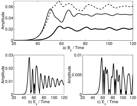
The grows exponentially at the rate until in and at until in the . The maximum linear growth rate obtained from a cold fluid model is [20]. The measured growth rate is reduced compared to in particular for the simulation by thermal effects, which cause damping at large . The amplitude of saturates and remains almost constant in all simulations after . The saturation amplitudes are , and . The magnetic trapping mechanism sets in, when is comparable to the magnetic bounce frequency in physical units [14]. The for the measured growth rates above are for and for and . The agreement is excellent for the simulation , but the increase of in the simulations compared to that in does not change . What we find instead is, that .
The grows when has reached a large amplitude and the growth rate of is twice that of , as it has previously been reported [18, 21]. The in the simulation oscillates between a peak value and zero, whereas we find damped oscillations around a steady state value in after . The peak amplitude of in the simulation exceeds that of by the factor 3 and that in is even stronger (not shown).
3.1 Simulation
The evolution of the electromagnetic fields and of the related electron phase space is now examined in more detail. Figure 2 shows the relevant fields in space and time for the simulation . It also compares the spatial distributions of and at the time , when the FI saturates.
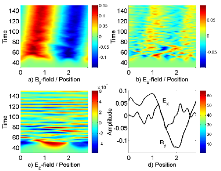
The simulation box fits one oscillation of at any fixed time after the saturation, but the more rapid oscillations along during indicate that at least initially several modes are competing. Eventually, the current channels merge and form a steady state distribution in 1D [14, 21]. The magnetic field structure slowly convects to larger . The phase speed of this structure is constant after and it amounts to . The oscillations of are more rapid than those of for any fixed . The maxima of after show a clear correlation with the structure of , because both convect with the same phase speed. The amplitudes of and show a possible correlation only at . The smaller filaments are merging to the larger one at this time, complicating the interpretation of the field correlation. The has the same spatial oscillation frequency as for any fixed and their phase is shifted by the expected . The amplitude of is significantly lower than that of . The oscillations of after show no pronounced structures.
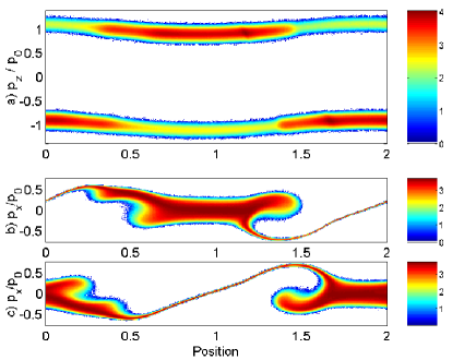
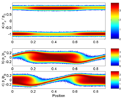
Figure 3 displays the phase space densities and at the times and . They show a significant modulation and the density maxima of both beams are shifted by at . The values of and vary by two orders of magnitude. The mean values for each beam show the same oscillatory modulation with as in Ref. [21]. The at also shows that several filaments develop. For example, a density maximum is found at and that is spatially correlated with a minimum at . The . The absolute minima of at and of at are also not shifted by . The smaller filaments cause the rapid spatial modulation of in Fig. 2. The electrons are heated up in by the saturation of the FI from an initial thermal spread of to a peak value of . The summation of over many filaments will give a distribution, that decreases exponentially over a wide range of [21].
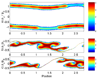
The supplementary movie 1 shows the 10-logarithmic and in the simulation . It demonstrates that only the core electrons in Fig. 3 remain spatially confined. This dense core population maintains in Fig. 2. The structures in in the movie 1, one of which occurs in Fig. 3e) at and , resemble phase space holes [28]. The potentials of these structures contribute to the , causing its rapid fluctuations in Fig. 2d). These phase space holes complicate the identification of the relation between in Fig. 2d) in addition to the ongoing merging of small filaments to larger ones.
3.2 Simulation
We reduce now the box length from to . The comparison of Fig. 4 with Fig. 2 reveals some similarities between the respective field evolutions. The structures in the saturated and fields are co-moving also in the simulation and they have here a phase speed . The and have the same spatial oscillation period when they saturate at , again shifted by . The does not show the spatial modulations with , which the in Fig. 2 does prior to its saturation at . Contrary to the Fig. 2d), the and the are obviously correlated in Fig. 4d). The whenever , which suggests the magnetic pressure gradient as the origin of . The dominant oscillations of in Fig. 4d) are in the and mode, respectively. The component evidences furthermore the presence of harmonics.
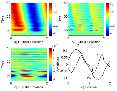
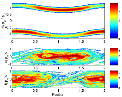
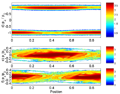
Figure 5 illustrates the phase space distributions and at the times and in the simulation . The density maxima are shifted by at both times and no further density maxima occur. The phase space structures of both beams at reveal a high degree of symmetry, evidencing a dominant single filament.
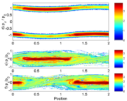
A second, independently developing filament would break such a symmetry as in the simulation . This is in line with the growth of in Fig. 4 that shows only a modulation with the wavenumber . The constant slope of in Fig. 4d) corresponds to a spatially uniform distribution of in Fig. 5b). The harmonics of in Fig. 4d) are related to the phase space structures at the filament boundaries. The at shows a heated electron population similar to that in Fig. 3. The dense electron component in is, however, cooler and it shows no vortex structures. The core populations of both beams in Fig. 5e,f) are not overlapping, as the current filaments do in the Fig. 3.
The supplementary movie 2 animates in time the 10-logarithmic phase space distributions and of the beam 1 in the simulation . The formation of the filaments is demonstrated. The phase space evolution shows that the distribution contains fewer vortices and that the vortices are spread out over a smaller interval of than in the simulation . The spatial modulation of of the beam 1 is also less pronounced. The plasma thus appears to be less turbulent than that in , which may explain the more obvious relation between and in Fig. 4 compared to the Fig. 2. The spatial width of the plasmon containing the dense bulk of the electrons of oscillates in time. The overlap of the filaments in Fig. 5e,f) is thus time dependent and related to the oscillating electrostatic field in Fig. 4b).
3.3 Simulation
The turbulence is reduced further, by decreasing the box length from to . We exploit this to examine quantitatively and in more detail the relation between the electric and magnetic fields and their effect on the particle trajectories. Figure 6 displays stationary field structures. The oscillates with the wavenumber in space. The oscillates with the wavenumber and it is practically undamped. Both fields display a persistent correlation. The component is damped in time and it is shifted by the phase relative to when the FI saturates. The damping of does not visibly influence the and , suggesting that is driven only during the growth phase of the FI and that it decouples upon saturation.
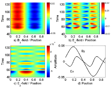
The fields show an excellent qualitative match between and when .
The force of the magnetic pressure gradient on a current is expressed as
| (4) |
The derivatives in the and the directions vanish in our 1D geometry, and . The magnetic pressure gradient force on the electrons can only be mediated through an electric field force along . This electric field for the normalized electron charge is then given by . The oscillates in Fig. 6 in space and time between and an extremum. The peak field moduli are most suitable for a comparison with , due to the high signal-to-noise ratio.
Figure 7a) displays the when the FI has just saturated and compares it with .
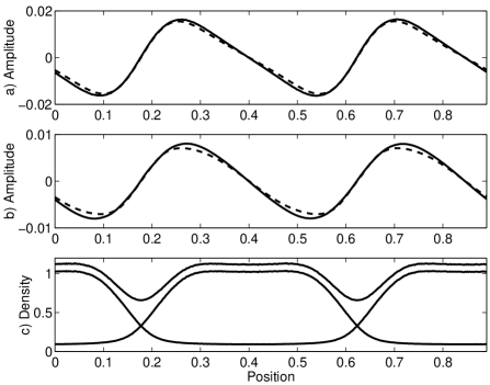
It turns out that at , when the peak amplitude of is reached. The electric field amplitudes can be averaged over the time interval to , for which the field structures do not convect and oscillate around a constant mean field, to give and . The and match in Fig. 7b). The magnetic pressure gradient is thus the origin of the electrostatic field. The system is oscillating around the equilibrium because our initial conditions did not correspond to a steady state configuration. The same oscillations of around a mean field as well as the correlation between and can also be observed in Fig. 2 and Fig. 4 at late times for the larger boxes. The correlates well with the in the simulations , although the curves do not match as accurately as in Fig. 7. This is due to the more turbulent plasma and because the convection of the structures imposes either constraints on the integration time or requires a transformation into a moving frame, the speed of which has to be estimated.
Figure 7c) shows the normalized number density distributions of the individual beams and also the summed distribution at . The spatial oscillation period of either or is , while that of the is . The phase space structures of electron phase space holes in an unmagnetized plasma would have the same periodicity as the electrostatic field [28].
Figure 8 shows the phase space distribution of the electrons in simulation at the times .
The are practically unchanged along the x-direction. A spatial modulation is caused by the -drift, the speed of which is given by the product of and in our 1D simulations. The amplitudes of and of both increase according to the Figs. 2, 4 and 6 as the filaments get larger and, hence, the drift speed contribution to . The amplitudes of in the simulations are several times the one in the simulation and their drift electric fields are larger. The simulation boxes are also longer. The electrostatic potentials in the simulations thus exceed by far that in the simulation and the electrons can reach higher kinetic energies. Consequently, the spread in of the phase space distributions of both beams in the simulation is less than half of that in the simulations at .
The supplementary movie 3 animates in time the evolution of the 10-logarithmic distributions and in the simulation . The evidences that the electrons are re-distributed along , but not along . The electron flow along oscillates. The after the saturation of the FI has a dense electron core, which rotates in the -plane around . Two vortices in the dense electron core, presumably electron phase space holes, are convected with this rotating flow.
All simulations evidence that a core of cool electrons is spatially confined. Their circular phase space motion in the movies around the equilibrium points with , for example in the movie 3, furthermore reveals, that they are trapped by an electrostatic potential in the plane. We consider the quasi-equilibrium established in the simulation after the FI has saturated. We calculate and for the simulation . We integrate both fields from to , when the equilibrium is established. The weak modulation of and thus of the CPs in allows us to estimate the drift electric field as and the total electric field . The average potentials with the indices are calculated from these fields and is set such that . The potentials are expressed in Volts, allowing a straightforward comparison with the particle kinetic energies. The average fields and potentials are displayed by Fig. 9.
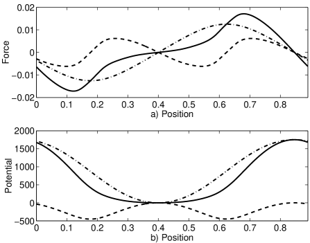
The electric fields are such that destabilizes the equilibrium position , because the negative close to accelerates the electron in the positive direction and the positive close to in the negative direction. The is confining the electrons around . The for and is thus a confining force. However, the electron acceleration at is decreased and increased at larger . This is reflected also by the potentials. The magnetic potential invoked by Ref. [14] is dominant. However, the electrostatic field flattens the bottom of the potential and steepens the walls. This modified potential results in a bouncing time of electrons that differs from that in Ref. [14]. The asymmetry of the potential close to the stable equilibrium of the beam 1 and the stable equilibrium of the beam 2 arises from the dependence of on the beam velocity. The velocity is for beam 1 and for beam 2. The , on the other hand, acts on both beams in the same way.
The CPs of the beam 1 should follow almost straight paths close to and they should be rapidly reflected for . The potential difference 1700 V in the simulation should trap electrons with speeds up to . This matches the momentum spread of the cool core population in movie 3 or Fig. 8. The oscillations of in Fig. 6 explain the periodic release of electrons from this cool core seen in the movie 3 and the oscillatory force imposed on the electrons by contributes to their heating.
The trajectories of two CPs in the confined structure of beam 1 are followed in time in Fig. 10 in order to compare their dynamics to that expected from .
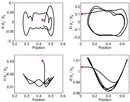
The red circle denotes the time, when the CPs start interacting with the fields and the trajectories are followed until . The CP 1 has a low initial modulus of and CP 2 a high one. Both CPs follow straight paths in the interval , in which in Fig. 9 is small. The phase space path of the faster CP 2 is smoother than that of CP 1. The low speed of CP 1 implies a long crossing time of the interval with a low modulus of and the CP 1 experiences several oscillation cycles of . The simultaneous action after the saturation of the FI of the quasi-stationary and the oscillatory , which both vary in space, implies that the electron acceleration is a function of the position and of the phase of relative to . This phase-dependence results in a randomization of the particle trajectories, contributing to the plasma heating. The faster CP 2 crosses the bottom of the potential more rapidly and it experiences lower relative speed changes by the . The particles are reflected outside the interval by the . Both CPs are trapped because their speed is less than that required to overcome .
The -fields are weak but not negligible. A comparison of the Figs. 2, 4 and 6 demonstrates, that its time-evolution depends on the box length. The grows in all simulations prior to the saturation of the FI and its phase is shifted by relative to . It is thus pumped through Ampere’s law by the growth of . The initial, low-frequency oscillations of with damp out in all simulations. They are replaced in the simulations by faster oscillations that have and . This is not the case for the in the simulation . The power spectrum of reveals the origins of the damping of the low-frequency modes and of the growth of the high-frequency modes. This power spectrum is obtained by Fourier transforming over the full box and simulation time. The power spectrum , which we plot for the simulations in Fig. 10.
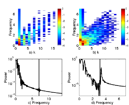
The reveals the following for the simulation . The spectrum of consists of the fundamental mode at and of secondary waves at with j=1+2n and . The modes with the are not harmonics of . They can thus not originate from a self-interaction of or from a coupling of with , which has also . It appears that is interacting with the mode of and, possibly, also with . The power spectrum is spread out in frequency, because initially grows exponentially and is thus not monochromatic. The can couple to the fast extraordinary (X-)mode with the same polarization. Its frequency in physical units at is high for the simulation due to the high of this simulation and no power is transfered from the low-frequency turbulence to the high-frequency fast X-mode. The transient oscillations of in the simulation damp out.
As we go from to the frequency of the fast X-mode at is lowered by a factor 2.25. Figure 11 evidences that now wave energy is coupled into the fast X-mode at . This pumping also transfers wave power to the mode with . This may be achieved by a parametric interaction of the low-frequency mode at and the high-frequency mode at . The frequency spread of the initial modes implies, that it is not necessary to fulfill exactly the frequency and wavenumber conservation of the 3-wave interaction. The fast X-modes are linearly undamped, explaining the persistent high-frequency oscillations of in the Figs. 2 and 4.
4 Discussion
In this work we have examined in detail the saturation of the electron beam filamentation instability (FI) with one-dimensional PIC simulations. The one-dimensional geometry implies that we can not model the FI beyond its saturation, because the filament merging is excluded [16]. However, we can readily distinguish between the electrostatic fields with their polarization vector along the simulation direction and the electromagnetic waves. The phase space distribution can also be sampled with a high statistical accuracy. We have modelled here only mobile electrons. The simulation compensates their charge by introducing an immobile positive charge background that cancels the electron charge.
The FI grows magnetic fields out of noise by a spatial separation of the currents of the, initially uniform, electron beams. A broad wavenumber spectrum is destabilized and the amplitudes of the individual filamentation modes grow aperiodically and exponentially. The magnetic field amplitude can not grow indefinitely. The magnetic amplitude saturates, once the bouncing frequency of the electrons in the magnetic potential becomes comparable to the growth rate of the instability [14]. More recently, it has been pointed out that the electrostatic fields upon saturation may not be negligible [18]. These electrostatic fields have been connected qualitatively to the magnetic pressure gradient [20, 21]. The observation, that the saturation of the FI is qualitatively unchanged by a beam-aligned magnetic field, has led to the suggestion in Ref. [20], that it is not the magnetic trapping but the electrostatic fields that quench the instability. This is, because the bouncing frequency of electrons depends on the strength of the flow-aligned magnetic field, while the electrostatic field does not; the pressure gradient of a uniform magnetic field vanishes and leaves unchanged the electrostatic field.
The electron beams in our simulations have been equally dense and cool. The beams counter-propagated at a non-relativistic speed orthogonally to the simulation direction. Picking a box length comparable to the filament size has allowed us to obtain a quasi-monochromatic wave spectrum and one pair of filaments. We have demonstrated quantitatively, that the electrostatic field is indeed driven by the magnetic pressure gradient. The initial conditions we have used here do not represent a steady state and the saturated plasma oscillates around its equilibrium state. The amplitude of the electrostatic field oscillates around the mean value, which is expected from the magnetic pressure gradient. We have demonstrated this for the small filament. Small means here, that no sub-structures can form because thermal effects [18, 29] limit the maximum unstable wavenumber. We have quantified the relative importance of the electrostatic field and of the magnetic field. The electrostatic field is comparable in strength to the drift electric field and both are thus relevant for the saturation of the FI and for the selected plasma parameters. The electrostatic field oscillates in space twice as fast as the magnetic one. Its effect is to reduce the force on the electrons close to the equilibrium point of the respective filament and to increase it farther away from it. The effective potential obtained from a summation of the magnetic pressure-driven electrostatic field and of the drift electric field is thus not a cosine.
The electrons can move almost freely through the potential well and are reflected at a relatively thin layer, as we have demonstrated for two representative computational particles. The effective potential is not symmetric with respect to both filaments. This is, because the drift electric field depends on the beam flow direction, while the magnetic pressure-driven electric field acts on all electrons the same way. The wall of the potential that is confining one filament is located well inside the potential well of the second filament. Filaments thus remain only separated if they have opposite beam flow directions, through which they can overlap without merging. This effective potential will also accelerate ions [18]. This ion acceleration is, however, exaggerated in 1D simulations where the potential is stationary in space. The filaments merge in higher-dimensional simulations and the potentials are not longer stationary. We have thus deliberately omitted to consider ion effects.
The electrons are heated up when the potential grows and also by their simultaneous interaction with the oscillatory electric field and the steady magnetic field. A dense and spatially confined electron population (plasmon) maintains the current responsible for the magnetic field after the heating has taken place. A hot electron population overcomes the potential well and presumably contributes to the quenching of the FI, which can be suppressed by a high temperature orthogonal to the beam flow direction [29].
We have then assessed the impact of the filament size on its dynamics. The probability distribution for the filament size has been sampled using a long one-dimensional simulation box in Ref. [21]. We have examined here two other filaments, the size of which we have selected according to the probability distribution. The size of the medium filament is close to the most common size. The large filament has a size close to the maximum observed one. Larger filaments can only form, if filaments merge in higher-dimensional systems [16, 23] because the growth rate of the FI decreases, as we go to smaller wavenumbers. Long waves are then outgrown by shorter waves. The electrostatic fields of the medium and the large filament have been correlated with the magnetic field after the FI has saturated and they have oscillated around an equilibrium value. This equilibrium value is close to the magnetic pressure gradient-driven field, as for the small filament. We have not shown it, because the fit is not as accurate as for the small filament, due to the drift of the structure and the increased levels of turbulence. The sub-structure, i.e. the merging of smaller filaments in the large filament, prior to the saturation of the FI has furthermore prevented a clear correlation of the electrostatic with the magnetic field at the saturation time. Both the medium and large filaments propagated after they have saturated, even though the phase speed of the waves driven by the FI is zero. The speed has, however, been less than the initial beam thermal speed. A filament can be accelerated by the saturation of the FI. Any net momentum of the hot and untrapped electron population must be balanced by an oppositely directed net momentum of the trapped electrons. The electromagnetic fields are tied to the trapped electrons and convect with the plasmons. The direction of the convection is random. The movie in Ref. [21] shows that different convection speeds of neighboring filaments result in their spatial oscillation rather than in a convection.
The mean momentum along the beam flow direction has been spatially modulated. Our comparative study of three filament sizes has shown that the magnetic field amplitude and the electrostatic field amplitude both increase with the filament size. They modulate the mean velocity of the beam through the -force. This modulation thus increases with the filament size, explaining the observation in Ref. [23] that trapped electrons reach increasingly higher speeds as the filaments merge.
The magnetic field has varied linearly in space over wide spatial intervals in all case studies. A magnetic field amplitude with a constant gradient results also in a magnetic pressure-driven electric field with a constant gradient. The Fourier transform over space of a curve with a constant gradient results in a power-law spectrum. This is observed also in longer- and in higher-dimensional simulation boxes [21, 23, 30].
We have examined the electric field component along the beam flow direction. Its wavenumber, the phase shift relative to the magnetic field and that it grows during the linear phase of the FI implies that it is driven through Ampere’s law. These low-frequency oscillations are transient modes and they damp out. However, we have confirmed here a previous observation [18], that the fast extraordinary mode is pumped by this wave component. We could observe this only for the two large filaments. The finite box size introduces a discrete wave spectrum. The larger the box length, the lower the frequency of the electromagnetic mode. The frequency has been low enough in the large simulation boxes to absorb wave energy from the low-frequency turbulence. The discrete wave spectrum is, however, a finite box (numerical) effect.
4.1 Acknowledgments
The authors acknowledge the financial support by an EPSRC Science and Innovation award, by the visiting scientist programme of the Queen’s University Belfast, by Vetenskapsrådet and by the Deutsche Forschungsgemeinschaft. The Swedish HPC2N computer center has provided the computer time and support.
References
References
- [1] Yang T Y B, Gallant Y, Arons J and Langdon A B 1993 Phys. fluids B 5 3369
- [2] Petri J and Kirk J G 2007 Plasma Phys. Controll. Fusion 49 297
- [3] Karlicky M, Nickeler D H and Barta M 2008 Astron. Astrophys. 486 325
- [4] Stockem A, Lerche I and Schlickeiser R 2006 Astrophys. J. 651 584
- [5] Niemiec J, Pohl M, Stroman T and Nishikawa K 2008 Astrophys. J. 684 1174
- [6] Tabak M et al. 1994 Phys. Plasmas 1 1626
- [7] Macchi A et al. 2003 Nucl. Fusion 43 362
- [8] Campbell R B, Kodama R, Mehlhorn T A, Tanaka K A and Welch D R 2005 Phys. Rev. Lett. 94 055001
- [9] Woolsey N C et al. 2001 Phys. Plasmas 8 2439
- [10] Startsev E A, Davidson R C and Qin H 2007 Phys. Plasmas 14 056705
- [11] Startsev E A and Davidson R C 2003 Phys. Plasmas 10 4829
- [12] Weibel E S 1959 Phys. Rev. Lett. 2 83
- [13] Yoon P H 2007 Phys. Plasmas 14 024504
- [14] Davidson R C, Wagner C E, Hammer D A and Haber I 1972 Phys. Fluids 15 317
- [15] Lazar M, Schlickeiser R and Shukla P K 2006 Phys. Plasmas 13 102107
- [16] Lee R and Lampe M 1973 Phys. Rev. Lett. 31 1390
- [17] Davidson R C, Hammer D A, Haber I and Wagner C E 1972 Phys. Plasmas 15 317
- [18] Califano F, Cecchi T and Chiuderi C 2002 Phys. Plasmas 9 451
- [19] Honda M, Meyer-ter-Vehn J and Pukhov A 2000 Phys. Rev. Lett. 85 2128
- [20] Stockem A, Dieckmann M E and Schlickeiser R 2008 Plasma Phys. Controll. Fusion 50 025002
- [21] Rowlands G, Dieckmann M E and Shukla P K 2007 New J. Phys. 9 247
- [22] Medvedev M V, Fiore M, Fonseca R A, Silva L O and Mori W B 2005 Astrophys. J. 618 L75
- [23] Dieckmann M E, Lerche I, Shukla P K and Drury L O C 2007 New J. Phys. 9 10
- [24] Sakai J I, Schlickeiser R and Shukla P K 2004 Phys. Lett. A 330 384
- [25] Bret A, Gremillet L and Bellido J C 2007 Phys. Plasmas 14 032103
- [26] Dawson J M 1983 Rev. Mod. Phys. 55 403
- [27] Eastwood J W 1991 Comput. Phys. Commun. 64 252
- [28] Eliasson B and Shukla P K 2006 Phys. Rep. 422 225
- [29] Bret A, Firpo M C and Deutsch C 2005 Phys. Rev. E 72 016403
- [30] Frederiksen J T, Hededal C B, Haugbolle T and Nordlund A 2004 Astrophys. J. 608 L13