One and two-center processes in high-order harmonic generation in diatomic molecules: influence of the internuclear separation

Abstract

We analyze the influence of different recombination scenarios, involving one or two centers, on high-order harmonic generation (HHG) in diatomic molecules, for different values of the internuclear separation. We work within the strong-field approximation, and employ modified saddle-point equations, in which the structure of the molecule is incorporated. We find that the two-center interference patterns, attributed to high-order harmonic emission at spatially separated centers, are formed by the quantum interference of the orbits starting at a center $C_{j}$ and finishing at a different center $C_{\nu}$ in the molecule with those starting and ending at a same center $C_{j}.$ Within our framework, we also show that contributions starting at different centers exhibit different orders of magnitude, due to the influence of additional potential-energy shifts. This holds even for small internuclear distances. Similar results can also be obtained by considering single-atom saddle-point equations and an adequate choice of molecular prefactors.

I Introduction

Molecules in strong laser fields have attracted a great deal of attention in the past few years. Indeed, strong-field phenomena, such as high-order harmonic generation, above-threshold ionization, and nonsequential double ionization, may be used as tools for measuring and even controlling dynamic processes in such systems with attosecond precision Scrinzi2006 . This is a direct consequence of the fact that the physical mechanisms behind such phenomena take place within a fraction of the period of the laser field. For a typical, titanium-sapphire laser used in experiments, whose period is of the order $\tau\sim 2.7\mathrm{fs}$, this means hundreds of attoseconds.

Explicitly, such phenomena can be described as the laser-assisted rescattering or recombination of an electron with its parent ion, or molecule tstep . At an instant $t^{\prime},$ this electron reaches the continuum through tunneling or multiphoton ionization. Subsequently, it propagates in the continuum, being accelerated by the external field. Finally, it is driven back towards its parent ion, or molecule, with which it recombines or rescatters at a later instant $t$. In the former case, the electron kinetic energy is converted in a high-energy, XUV photon, and high-order harmonic generation (HHG) takes place hhgsfa . In the latter case, one may distinguish two specific scenarios: The electron may suffer an elastic collision, which will lead to high-order above-threshold ionization (ATI) atisfa , or transfer part of its kinetic energy to the core, and release other electrons. Hence, laser-induced nonsequential double (NSDI), or multiple ionization (NSMI) will occur.

For molecules, there exist at least two centers with which the electron may recombine or rescatter. This leads to interference patterns which are due to photoelectron or high-harmonic emission at spatially separated centers, and which contain information about its specific structure. In the simplest case of diatomic molecules, such patterns have been described as the microscopic counterpart of a double-slit experiment doubleslit ; KB2005 .

A legitimate question is what sets of electron orbits are most relevant for the two- or many-center interference patterns. To understand this issue is a first step towards controlling such processes by, for instance, an adequate choice of the shape and polarization of the external field. In the specific case of diatomic molecules, the electron may start and return to the same center $C_{j}$, or leave from a center $C_{j}$ and return to a center $C_{\nu},\nu\neq j(j=1,2)$. Hence, in total, there exist four possible processes that contribute to the yield. Recently, these processes have been addressed in several studies, for above-threshold ionization Usach2006 ; HBF2007 ; DM2006 ; BCCM2007 ; Milos2008 , high-order harmonic generation KBK98 ; KB2005 ; PRACL2006 ; F2007 and nonsequential double ionization F2008 . The vast majority of these studies has been performed using semi-analytical methods, in the context of the strong-field approximation. In this framework, the transition amplitude can be written as a multiple integral with a slowly varying prefactor and a semiclassical action. The structure of the molecule may be either incorporated in the former MBBF00 ; Madsen ; Usachenko ; Kansas ; JMOCL2006 ; FSLY2008 , or in the latter Usach2006 ; HBF2007 ; Milos2008 ; KBK98 ; PRACL2006 ; F2007 ; F2008 . On a more specific level, when solving these integrals employing saddle-point methods, it is possible to draw a space-time picture of the laser-assisted rescattering or recombination process in question, and establish a direct connection to the orbits of a classical electron in a strong laser field orbitshhg . By incorporating the structure of the molecule in the action, one obtains modified saddle-point equations which gives the one-or two-center scenarios.

In a previous publication F2007 , we have addressed this issue to a large extent for high-order harmonic generation, within the Strong-Field Approximation (SFA).  Our results suggested that the maxima and minima observed in the spectra were due to the quantum interference of the processes in which the electron leaves and returns to a specific center $C_{j}$ in the molecule with those in which it leaves from $C_{j}$, but returns to a different center $C_{\nu}.$ There exist, however, a few ambiguities as far as the interpretation of our findings is concerned. For instance, in the length-gauge formulation of the SFA, we found additional potential energy shifts, which depend on the field strength $E(t)$ and in the internuclear separation $R.$ These shifts led to a strong suppression of tunnel ionization at one of the centers. This could have led to the conclusion that the interference between other processes were not relevant for the patterns in the spectra.

In this proceeding, we investigate the role of the one and two-center recombination scenarios in more detail. In particular, we analyze the above-mentioned potential energy shifts and their influence on the spectra,  for smaller internuclear distances than those taken in F2007 . We also provide an alternative interpretation of the results encountered, based on effective prefactors and single-atom saddle-point equations.

This paper is organized as follows. In Sec. II, we briefly recall the strong-field approximation HHG transition amplitudes. Thereby, we consider the situation for which the structure of the molecule is either incorporated in the prefactor (Sec. II.2 ), or in the semiclassical action (Sec. II.3). Subsequently (Sec. III), we analyze the role of the different scenarios, involving one and two centers, in the high-harmonic spectra, either solving the modified saddle-point equations (Sec. III.1), or mimicking the quantum-interference between different sets of orbits by an adequate choice of prefactors (Sec. III.2). Finally, in Sec. IV we outline the main conclusions of this work.

II Transition amplitudes

II.1 General expressions

As a starting point, we will underline our main assumptions with regard to the diatomic bound-state wave functions. We consider frozen nuclei, the linear combination of atomic orbitals (LCAO) approximation, and homonuclear molecules. Under these assumptions, the electronic bound-state wave function reads

$$\psi_{0}(\mathbf{r})=C_{\psi}(\phi_{0}(\mathbf{r}-\mathbf{R}/2)+\epsilon\phi_{0}(\mathbf{r}+\mathbf{R}/2)),$$ (1)

where $\epsilon=\pm 1,$ $C_{\psi}=1/\sqrt{2(1+\epsilon S(\mathbf{R})},$ with

$$S(\mathbf{R})=\int\left[\phi_{0}(\mathbf{r}-\mathbf{R}/2)\right]^{\ast}\phi_{0}(\mathbf{r}+\mathbf{R}/2)d^{3}r$$ (2)

The positive and negative signs for $\epsilon$ denote symmetric and antisymmetric orbitals, respectively. For simplicity, unless otherwise stated we will consider parallel-aligned molecules.

The SFA transition amplitude for high-order harmonic generation reads, in the specific formulation of Ref. hhgsfa and in atomic units,

$$M^{(\Omega)} = i\int_{-\infty}^{\infty}dt\int_{-\infty}^{t}~{}dt^{\prime}\int d^{3}kd_{\mathrm{rec}}^{\ast}(\mathbf{\tilde{k}}(t))d_{\mathrm{ion}}(\mathbf{\tilde{k}}(t^{\prime}))$$ (3)

$$\exp[iS(t,t^{\prime},\Omega,\mathbf{k})]+c.c.,$$

with the action

$$S(t,t^{\prime},\Omega,\mathbf{k})=-\frac{1}{2}\int_{t^{\prime}}^{t}[\mathbf{k}+\mathbf{A}(\tau)]^{2}d\tau-I_{p}(t-t^{\prime})+\Omega t$$ (4)

and the prefactors $d_{\mathrm{rec}}(\mathbf{\tilde{k}}(t))=\left\langle\mathbf{\tilde{k}}(t)\right|\mathbf{r}.\mathbf{e}_{x}\left|\psi_{0}\right\rangle$ and $d_{\mathrm{ion}}(\mathbf{\tilde{k}}(t^{\prime}))=\left\langle\mathbf{\tilde{k}}(t^{\prime})\right|H_{\mathrm{int}}\mathbf{(}t^{\prime}\mathbf{)}\left|\psi_{0}\right\rangle.$ Thereby $\mathbf{r}$, $\mathbf{e}_{x}$, $H_{\mathrm{int}}\mathbf{(}t^{\prime}\mathbf{),}$ $I_{p},$ and $\Omega$ give the dipole operator, the laser-polarization vector, the interaction with the field, the ionization potential, and the harmonic frequency, respectively. The explicit expressions for $\mathbf{\tilde{k}}(t)$ are gauge dependent, and will be provided below. Physically, Eq. (3) describes a process in which an electron, initially in a field-free bound-state $\left|\psi_{0}\right\rangle$, is coupled to a Volkov state $\left|\mathbf{\tilde{k}}(t^{\prime})\right\rangle$ by the interaction $H_{\mathrm{int}}\mathbf{(}t^{\prime}\mathbf{)}$ of the system with the field. Thereafter, it propagates in the continuum and is driven back towards its parent ion, or molecule. At a time $t,$ it recombines, emitting high-harmonic radiation of frequency $\Omega.$

The above-stated transition amplitude may be either solved numerically, or employing saddle-point equations. In this work, we employ the latter method and the specific uniform approximation discussed in Ref. atiuni . Explicitly, these equations are given by the condition that the semiclassical action be stationary, i.e., that $\partial_{t}S(t,t^{\prime},\Omega,\mathbf{k})=\partial_{t^{\prime}}S(t,t^{\prime},\Omega,\mathbf{k})=0$ and $\partial_{\mathbf{k}}S(t,t^{\prime},\Omega,\mathbf{k})=\mathbf{0.}$

For a single atom placed at the origin of the coordinate system, this leads to

$$\left[\mathbf{k}+\mathbf{A}(t^{\prime})\right]^{2}=-2I_{p},$$ (5)

$$\int_{t^{\prime}}^{t}d\tau\left[\mathbf{k}+\mathbf{A}(\tau)\right]=0,$$ (6)

and

$$2(\Omega-I_{p})=\left[\mathbf{k}+\mathbf{A}(t)\right]^{2}.$$ (7)

Eq. (5) gives the conservation of energy at the instant $t^{\prime}$of ionization, and has no real solution. Indeed, the time $t^{\prime}$ will possess a non-vanishing imaginary part. This is due to the fact that tunneling is a process which has no classical counterpart. In the limit $I_{p}\rightarrow 0,$ corresponds to the physical situation of a classical electron reaching the continuum with vanishing drift velocity. Eq. (6) expresses the fact that the electron propagates in the continuum from $t^{\prime}$ to $t,$ when it returns to the site of its release. Eq. (7) yields the conservation of energy at the recombination instant $t,$ when the kinetic energy of the returning electron is converted into high-order harmonic radiation.

One should note that the transition amplitude (3) is gauge dependent FKS96 ; PRACL2006 . Firstly, the interaction Hamiltonians $H_{\mathrm{int}}(t^{\prime})$, which are present in $d_{\mathrm{ion}}(\mathbf{\tilde{k}}(t^{\prime}))$, are different in the length and velocity gauges. Furthermore, in both velocity- and length-gauge formulations, field-free bound states are taken, which are not gauge equivalent. Therefore, different gauge choices will yield different interference patterns PRACL2006 ; DM2006 ; Madsen ; Usachenko ; F2007 ; SSY2007 . This problem has been overcome to a large extent by considering field-dressed bound states, as a dressed state in the length gauge is gauge-equivalent to a field-free bound state in the velocity gauge, and vice-versa (for details see dressedSFA ; F2007 ; DM2006 ).

II.2 Double-slit interference condition

The matrix element $d_{\mathrm{rec}}(\mathbf{\tilde{k}})=\left\langle\mathbf{\tilde{k}}\right|\mathbf{r}\cdot\mathbf{e}_{x}\left|\psi_{0}\right\rangle$ is then given by

$$d_{\mathrm{rec}}^{(b)}(\mathbf{\tilde{k}})=\frac{2iC_{\psi}}{(2\pi)^{3/2}}\left[-\cos(\vartheta)\partial_{p_{x}}\phi(\mathbf{\tilde{k}})+\frac{R_{x}}{2}\sin(\vartheta)\phi(\mathbf{\tilde{k}})\right],$$ (8)

for bonding molecular orbitals (i.e., $\epsilon>0),$ or

$$d_{\mathrm{rec}}^{(a)}(\mathbf{\tilde{k}})=\frac{2C_{\psi}}{(2\pi)^{3/2}}\left[\sin(\vartheta)\partial_{p_{x}}\phi(\mathbf{\tilde{k}})-\frac{R_{x}}{2}\cos(\vartheta)\phi(\mathbf{\tilde{k}})\right],$$ (9)

in the antibonding case (i.e., $\epsilon<0),$ with $\vartheta=\mathbf{\tilde{k}}\cdot\mathbf{R}/2.$ In the above-stated equations, $R_{x}$ denotes the projection of the internuclear distance along the direction of the laser-field polarization.

In Eqs. (8) and (9), the terms with a purely trigonometric dependence on the internuclear distance yield the double-slit condition in doubleslit . The maxima and minima in the spectra which are caused by this condition are expected to occur for

$$\mathbf{\tilde{k}}\cdot\mathbf{R}=2n\pi\text{ and }\mathbf{\tilde{k}}\cdot\mathbf{R}=(2n+1)\pi,$$ (10)

respectively, for bonding molecular orbitals (i.e., $\epsilon>0).$ For antibonding orbitals, the maxima occur for the odd multiples of $\pi$ and the minima for the even multiples. In the length and velocity gauges $\mathbf{\tilde{k}}(\tau)=\mathbf{k}+\mathbf{A}(\tau)$ and $\mathbf{\tilde{k}}(\tau)=\mathbf{k}$, where $\tau=t,t^{\prime}$, respectively.

The remaining terms grow linearly with $R_{x}$, and are an artifact of the strong-field approximation, due to the fact that the continuum states and the bound states are not orthogonal in the context of the strong-field approximation JMOCL2006 ; F2007 ; SSY2007 . For that reason, they will be neglected here (for rigorous justifications see DM2006 ; SSY2007 ).

In the length gauge, $d_{\mathrm{rec}}(\mathbf{\tilde{k}}(t))=d_{\mathrm{ion}}(\mathbf{\tilde{k}}(t^{\prime}))$, with $\ \mathbf{\tilde{k}}(t)=\mathbf{k}+\mathbf{A}(t),$ while in the velocity gauge,

$$d_{\mathrm{ion}}^{(b)}(\mathbf{\tilde{k}})=\frac{C_{\psi}[\mathbf{k}+\mathbf{A}(t^{\prime})]^{2}}{(2\pi)^{3/2}}\cos(\vartheta)\phi(\mathbf{\tilde{k}}),$$ (11)

or

$$d_{\mathrm{ion}}^{(a)}(\mathbf{\tilde{k}})=-i\frac{C_{\psi}[\mathbf{k}+\mathbf{A}(t^{\prime})]^{2}}{(2\pi)^{3/2}}\sin(\vartheta)\phi(\mathbf{\tilde{k}}),$$ (12)

with $\mathbf{\tilde{k}}(t)=\mathbf{k,}$ for bonding and antibonding molecular orbitals, respectively. The simplest and most widely adopted MBBF00 ; Madsen ; Usachenko ; KB2005 ; DM2006 ; JMOCL2006 procedure is to employ the prefactors $d_{\mathrm{ion}}(\mathbf{\tilde{k}})$   and $d_{\mathrm{rec}}(\mathbf{\tilde{k}})$ and the single-atom saddle-point equations (5)-(7). In this case, we consider the origin, from which the electron leaves and returns, as the geometric center of the molecule.

II.3 Modified saddle-point equations

The prefactors $d_{\mathrm{ion}}^{(b)}(\mathbf{\tilde{k}})$ and $d_{\mathrm{rec}}^{(b)}(\mathbf{\tilde{k}})$ will now be exponentialized and incorporated in the action (for details, see PRACL2006 ; F2007 ). For the recombination matrix element, we take the expression

$$d_{\mathrm{rec}}^{(b)}(\mathbf{\tilde{k}})=-\frac{2iC_{\psi}}{(2\pi)^{3/2}}\left[\cos\left(\mathbf{\tilde{k}}\cdot\frac{\mathbf{R}}{2}\right)\partial_{\tilde{p}_{x}}\phi(\mathbf{\tilde{k}})\right],$$ (13)

for which the spurious term is $R_{x}$ is absent. In the expression for the antibonding case, the cosine term in (13) should be replaced by $\sin(\mathbf{\tilde{k}\cdot R}/2)$. Without loss of generality, the same procedure can also be applied to more complex orbitals.

This leads to the sum

$$M=\sum_{j=1}^{2}\sum_{\nu=1}^{2}M_{j\nu}$$ (14)

of the transition amplitudes

$$M_{j\nu} = \frac{C_{\psi}}{(2\pi)^{3/2}}\int_{0}^{t}dt^{\prime}\int dt\int d^{3}p\eta(\mathbf{k},t,t^{\prime})$$ (15)

$$\times\exp[iS_{j\nu}(\mathbf{k},\Omega,t,t^{\prime})],\$$

with $\eta(\mathbf{k},t,t^{\prime})=\left[\partial_{\tilde{p}_{x}}\phi(\mathbf{\tilde{k}}(t))\right]^{\ast}\partial_{\tilde{p}_{x}}\phi(\mathbf{\tilde{k}(}t^{\prime})).$ The terms $S_{j\nu}(\mathbf{k},\Omega,t,t^{\prime})$ correspond to a modified action, which incorporates the structure of the molecule. Explicitly, they read

$$S_{j\nu}(\mathbf{k},\Omega,t,t^{\prime})=S(\mathbf{k},\Omega,t,t^{\prime})+(-1)^{\nu+1}\xi(R,t,t^{\prime})$$ (16)

where $\xi(R,t,t^{\prime})=[\mathbf{\tilde{k}}(t)\mathbf{-}(-1)^{\nu+j}\mathbf{\tilde{k}}(t^{\prime})]\cdot\mathbf{R}/2$.

We will now compute the amplitudes $M_{j\nu}$ employing saddle-point methods. For this purpose, we will seek values for $t,t^{\prime}$ and $\mathbf{k}$ which satisfy the conditions $\partial_{\mathbf{k}}S_{j\nu}(\mathbf{k},\Omega,t,t^{\prime})=\mathbf{0},\ \partial_{t}S_{j\nu}(\mathbf{k},\Omega,t,t^{\prime})=0$ and $\partial_{t^{\prime}}S_{j\nu}(\mathbf{k},\Omega,t,t^{\prime})=0$. This leads to the saddle-point equations

$$\frac{[\mathbf{k}+\mathbf{A}(t^{\prime})]^{2}}{2}=-I_{p}+(-1)^{2\nu+j+1}\partial_{t^{\prime}}\mathbf{\tilde{k}}(t^{\prime})\cdot\mathbf{R}/2,$$ (17)

$$\int_{t^{\prime}}^{t}[\mathbf{k}+\mathbf{A}(s)]ds+(-1)^{\nu+1}\partial_{\mathbf{k}}\zeta=0,$$ (18)

with $\zeta=\left[\mathbf{\tilde{k}}(t)-(-1)^{j+\nu}\mathbf{\tilde{k}}(t^{\prime})\right]\cdot\mathbf{R}/2$ and

$$\frac{[\mathbf{k}+\mathbf{A}(t)]^{2}}{2}=\Omega-I_{p}+(-1)^{\nu}\partial_{t}\mathbf{\tilde{k}}(t)\cdot\mathbf{R}/2.$$ (19)

Eq. (17) corresponds to the tunnel ionization process, saddle-point equation (18) gives the condition that the electron returns to its parent molecule and Eq. (19) expresses the conservation of energy at the instant of recombination, in which the kinetic energy of the electron is converted into high-order harmonic radiation. The above-stated saddle-point equations depend on the gauge, on the center $C_{j}$ from which the electron was freed and on the center $C_{\nu}$ with which it recombines. Below we will have a closer look at specific cases. We will start by analyzing Eqs. (17) and (19), which, physically, correspond to the ionization and recombination process, respectively.

If the length gauge is chosen, both equations are explicitly written as

$$\frac{[\mathbf{k}+\mathbf{A}(t^{\prime})]^{2}}{2}=-I_{p}+(-1)^{2\nu+j}\mathbf{E}(t^{\prime})\cdot\mathbf{R}/2,$$ (20)

and

$$\frac{[\mathbf{k}+\mathbf{A}(t)]^{2}}{2}=\Omega-I_{p}+(-1)^{\nu+1}\mathbf{E}(t)\cdot\mathbf{R}/2,$$ (21)

respectively. For this specific formulation, there exist potential-energy shifts on the right-hand side, which depend on the external laser field $\mathbf{E}(\tau)(\tau=t,t^{\prime})$ and on the internuclear distance $\mathbf{R.}$ At the ionization or recombination times, depending on the center, they increase, or sink the potential-energy barrier through which the electron must tunnel, or the energy of the state with which it will recombine. In the specific case discussed here, there is a decrease in the barrier at $C_{2}$ and an increase at $C_{1}.$ Their meaning and existence altogether has raised considerable debate in the literature PRACL2006 ; DM2006 ; SSY2007 ; BCCM2007 .

In the velocity gauge, the saddle-point equations (17) and (19) read

$$\frac{[\mathbf{k}+\mathbf{A}(t^{\prime})]^{2}}{2}=-I_{p},$$ (22)

and

$$\frac{[\mathbf{k}+\mathbf{A}(t)]^{2}}{2}=\Omega-I_{p}.$$ (23)

These equations do not exhibit the above-mentioned potential-energy shifts, and resemble the saddle-point equations obtained for a single atom hhgsfa . Furthermore, if the limit $I_{p}\rightarrow 0$ is taken, Eq.(22) describes a classical particle reaching the continuum with vanishing drift momentum. In contrast, in the length gauge neither the classical limit nor the single-atom equations are obtained.

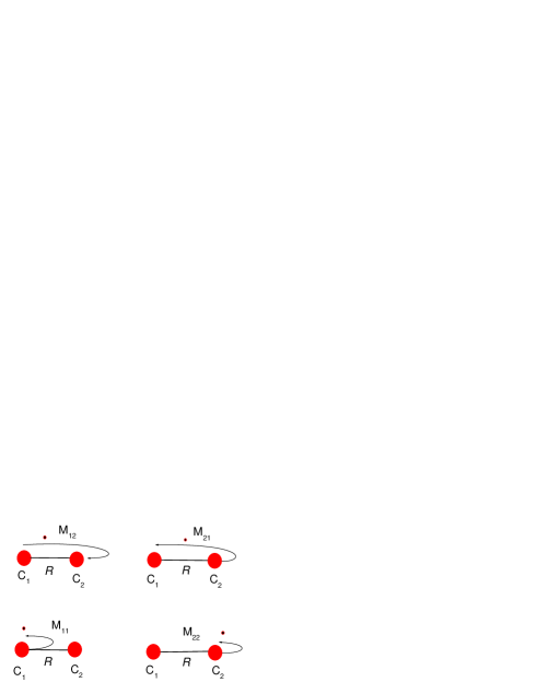
Figure 1: Schematic representation of the four possible recombination or rescattering scenarios described by Eq. (14). The centers $C_{1}$ and $C_{2}$ in the molecule, as well as the transition amplitudes $M_{j\nu}$ ($j,\nu=1,2$) are indicated in the figure.

We will now discuss the saddle-point equation (18) which gives the return condition. For both length and velocity gauges, one may distinguish two main scenarios: either the electron leaves and returns to the same center, i.e., $\nu=j$, or the electron is freed at a center $C_{j}$ and recombines with the other center $C_{\nu}$, $j\neq\nu,$ in the molecule. In the former and latter case, the return condition reads

$$\int_{t^{\prime}}^{t}[\mathbf{k}+\mathbf{A}(s)]ds=0,$$ (24)

or

$$\int_{t^{\prime}}^{t}[\mathbf{k}+\mathbf{A}(s)]ds+(-1)^{\nu+1}\mathbf{R}=0.$$ (25)

In Eq. (25), the index $\nu=2$ corresponds to the transition amplitudes $M_{12}$ (center $C_{1}$ to center $C_{2})$ and $M_{21}$ (center $C_{2}$ to center $C_{1})$, respectively. For clarity, the scenarios described above are summarized in Fig. 1.

III Quantum interference and different recombination scenarios

In the following we will discuss high-order harmonic spectra. For simplicity, we will consider that the electrons involved are initially bound in $1s$ states. This gives

$$\phi(\mathbf{\tilde{k}})\sim\frac{1}{[\mathbf{\tilde{k}}^{2}+2I_{p}]^{2}}$$ (26)

in the high-order harmonic prefactors $d_{\mathrm{ion}}^{(b)}(\mathbf{\tilde{k}})$ and $d_{\mathrm{rec}}^{(b)}(\mathbf{\tilde{k}})$.

In Fig. 2, we will commence by displaying the overall contributions, computed using the prefactors $d_{\mathrm{ion}}^{(b)}(\mathbf{\tilde{k}})$ and $d_{\mathrm{rec}}^{(b)}(\mathbf{\tilde{k}})$ and single-atom saddle point equations, instead of the modified saddle-point equations (17)-(19), for the length and velocity gauges. For comparison, the also present the contribution from all transition amplitudes $M_{j\nu}^{(\Omega)}$. In the present computations, we considered up to five pairs of orbits starting at the first half-cycle of the field, i.e., $0\leq t^{\prime}\leq T/2.$

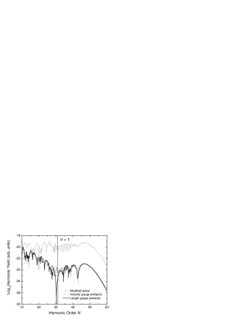
Figure 2: Spectra computed employing the single-atom orbits and two center prefactors, for the length and velocity gauges, compared to the length-gauge spectrum obtained employing modified saddle-point equations. We consider here the modified length form (13) of the dipole operator, which excludes the term with a linear dependence on $R_{x}$. The atomic system was approximated by the linear combination of $1s$ atomic orbitals with $I_{p}=0.57$ a.u.. The internuclear distance and the alignment angle are $R=2.068$ a.u., and $\theta=0,$ respectively. The driving field intensity and frequency are given by $I=3\times 10^{14}\mathrm{W/cm^{2}}$, and $\omega=0.057$ a.u., respectively. The interference minimum at $n=1$ is indicated by the vertical line in the figure. The difference in the orders of magnitude between the velocity and length gauge spectra is due to the different prefactors $d_{\mathrm{ion}}(\tilde{\mathbf{k}})$.

In the length gauge, the interference condition predicts interference extrema at $\Omega=I_{p}+n^{2}\pi^{2}/(2R^{2})$. For the parameters in the figure, this yields a minimum near $\Omega=31\omega$, for $n=1.$ Even though this minimum is shallower if modified saddle-point equations are taken, it can be easily identified.

In contrast, in the velocity gauge, the above-mentioned interference patterns are absent. This is due to the fact that the interference condition changes. The maxima and minima re now given by (10), with $\mathbf{k}$ instead of $\mathbf{\tilde{k}}=\mathbf{k}+\mathbf{A}(t).$ This will lead to interference extrema at harmonic frequency $\Omega=I_{p}+\left[n^{2}\pi^{2}/R^{2}+2n\pi A(t)/R+A^{2}(t)\right]/2.$ Roughly, if we assume that the vector potential at the electron return time is $A(t)\simeq 2\sqrt{U_{p}},$ this will correspond to $\Omega\sim 97\omega.$ This frequency lies far beyond the cutoff ( $\Omega\sim 47\omega)$, so that there will be a breakdown in the interference patterns F2007 ; SSY2007 . For this reason, in the following figures we will consider only the length-gauge situation.

III.1 Modified saddle-point equations

Subsequently, in Fig. 3, we present the contributions from the different recombination scenarios. In panel (a), the contributions from the topologically similar scenarios, involving only one or two centers, are depicted. We observe that the interference minimum mentioned in Fig. 1 is absent for both types of contributions.  At first sight, this seems to contradict the double-slit picture. In fact, for both $|M_{12}+M_{21}|^{2}$ and $|M_{11}+M_{22}|^{2},$ high-order harmonic emission at spatially separated centers takes place. Therefore, one would expect well-defined interference patterns to be present. One should note, however, that the potential energy shifts $\pm\mathbf{E}(t^{\prime})\cdot\mathbf{R}/2$ sink the potential barrier for the orbits starting at $C_{2}$ and increase the potential barrier for those starting at $C_{1}.$ Thus, the latter contributions are strongly suppressed and do not contribute significantly to the two-center interference.

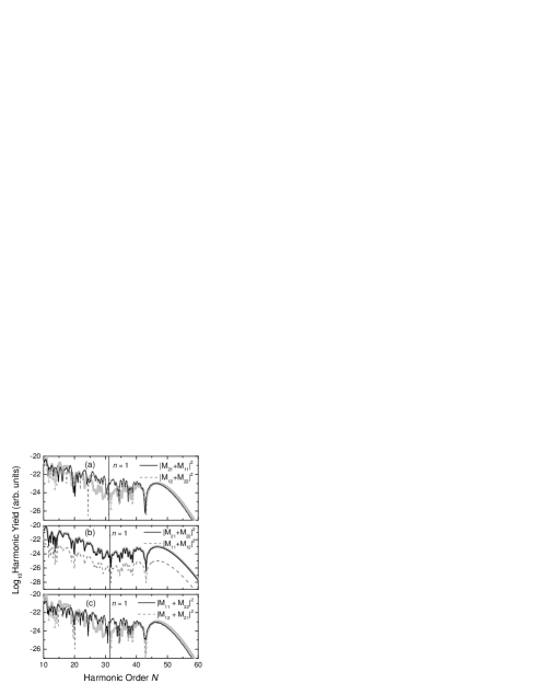
Figure 3: Contributions to the high-harmonic yield from the quantum interference between different types of orbits, for internuclear distance $R=2.068$ a.u. The remaining parameters are the same as in Fig. 2. Panel (a): Orbits involving similar scattering scenarios, i. e., $|M_{11}+M_{22}|^{2}$, and $|M_{12}+M_{21}|^{2}.$ Panel (b): Orbits starting at the same center, i.e., $|M_{11}+M_{12}|^{2}$ and $|M_{21}+M_{22}|^{2}.$ Panel (b): Orbits ending at the same center, i.e., $|M_{11}+M_{21}|^{2}$ and $|M_{12}+M_{22}|^{2}.$ For comparison, the full contributions $|M_{21}+M_{22}+M_{11}+M_{12}|^{2}$ are displayed as the light gray circles in the picture. The interference minimum at $n=1$ is indicated as the vertical line in the figure.

This is in agreement with panel (b), in which the contributions from the processes $|M_{jj}+M_{j\nu}|^{2}(j,\nu=1,2$ and $\nu\neq j)$ starting from the same center and ending at different centers are depicted. Therein, the contributions of the processes starting at $C_{2}$ are roughly two orders of magnitude larger than those starting at $C_{1}.$ This is due to the fact that the barrier through which the electron must tunnel in order to reach the continuum is much wider for the latter center. Furthermore, the two-center interference minimum near $\Omega=31\omega$ is present. This is expected, as the contributions from the centers $C_{1}$ and $C_{2}$ exhibit the same order of magnitude for both types of orbits.

Finally, in panel (c) we display the contributions $|M_{jj}+M_{\nu j}|^{2}$ from the processes starting at different centers and ending at the same center. In this case, the interference minimum is absent. This was expected for two reasons. First, for these orbits, there is no high-order harmonic emission taking place at spatially separated centers. Second, even if this were the case, the contributions from the orbits starting at $C_{2}$ are much stronger than those starting at $C_{1}$.

Since the potential energy shifts $\pm\mathbf{E}(t^{\prime})\cdot\mathbf{R}/2$ depend on the internuclear distance, it is legitimate to ask the question of whether, for small internuclear distances, a minimum is present in the contributions from the topologically similar scenarios. In Fig. 4, we considered such a situation. From the interference condition, we expect a minimum near $\Omega=69\omega$. This minimum is present for the overall contributions, and also for the processes $|M_{jj}+M_{j\nu}|^{2}(j,\nu=1,2$ and $\nu\neq j)$ starting from the same center and ending at different centers [Fig. 4.(a)]. It is however absent for the interference of topologically similar processes [Fig. 4.(b)]. This is due to fact that, even for this small internuclear distance, the orbits starting from $C_{2}$ lead to larger contributions than those starting from $C_{1}.$ Indeed, a closer look at Fig. 4.(a) shows that the contributions $|M_{11}+M_{12}|^{2}$ are roughly one order of magnitude smaller than $|M_{22}+M_{21}|^{2}$.

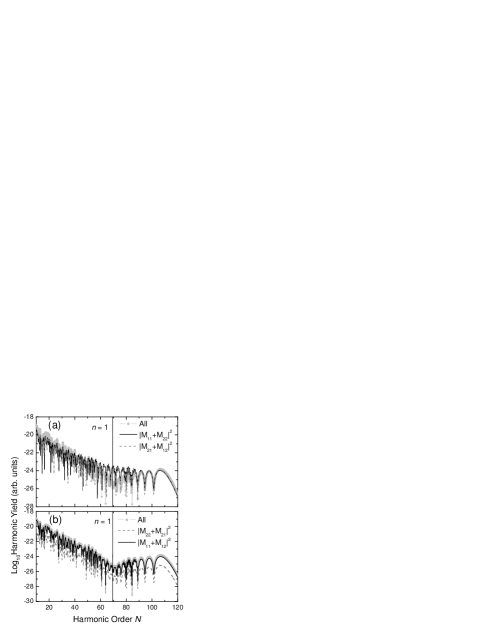
Figure 4: Contributions from different types of orbits to the high-harmonic yield, for internuclear distance $R=1.2$ a.u. and intensity $I=8\times 10^{14}\mathrm{W/cm}^{2}.$ The remaining parameters are the same as in the previous figures. Panel (a) gives the contributions from the topologically similar scattering scenarios, i. e., $|M_{11}+M_{22}|^{2}$, and $|M_{12}+M_{21}|^{2},$ and panel (b) of the orbits starting at the same center, i.e., $|M_{11}+M_{12}|^{2}$ and $|M_{21}+M_{22}|^{2}.$

Possibly, in order to obtain well-defined maxima and minima for the contributions of topologically similar scenarios, it would be necessary to reduce the internuclear distance even more. In this case, however, none of the assumptions adopted in this paper, such as the LCAO approximation, hold. In this context, it is worth noticing that the parameters adopted in Fig. 4 are also somewhat unrealistic, as far as this specific approximation is concerned. If, however, an alternative ionization pathway is provided, so that the electron may reach the continuum without the need of overcoming the potential-energy barriers, the contributions from the topologically similar scenarios may lead to well-defined patterns. Indeed, in previous work, we employed an additional attosecond-pulse train in order to release the electron in the continuum, and obtained an interference minimum in this case F2007 . We were, however, changing the physics of the problem by providing a different ionization mechanism. In the following, we will investigate the issue of the potential-energy shifts for this set of parameters, employing an alternative method.

III.2 Modified prefactors

On the other hand, the transition amplitudes $M_{j\nu}$ may also be grouped in such a way as to obtain effective prefactors. Such prefactors may then be related to the quantum interference of specific types of orbits. Hence, one may mimic the influence of the above-stated scenarios even if the single-atom saddle-point equations (5)-(7) are taken into account. For the symmetric combination of atomic orbitals considered here, there would be four different sets of prefactors, which are explicitly given by

$$d_{\mathrm{ion}}^{(j\nu)}(\mathbf{k},t,t^{\prime}) = 2\exp[(-1)^{j}i\mathbf{\tilde{k}}(t^{\prime})\cdot\mathbf{R}/2]$$

$$\times\cos[\mathbf{\tilde{k}}(t)\cdot\mathbf{R}/2]\eta(\mathbf{k},t,t^{\prime}),$$

$$d_{\mathrm{end}}^{(j\nu)}(\mathbf{k},t,t^{\prime}) = 2\exp[(-1)^{j}i[\mathbf{\tilde{k}}(t)\mathbf{+A}(t^{\prime})]\cdot\mathbf{R}/2]$$

$$\times\cos[\mathbf{k}\cdot\mathbf{R}/2]\eta(\mathbf{k},t,t^{\prime}),$$

$$d_{\mathrm{same}}(\mathbf{k},t,t^{\prime})=2\cos[\mathbf{[A}(t)-\mathbf{A}(t^{\prime})]\cdot\mathbf{R}/2]\eta(\mathbf{k},t,t^{\prime}),$$ (29)

and

$$d_{\mathrm{diff}}(\mathbf{k},t,t^{\prime}) = 2\cos[\mathbf{p}\cdot\mathbf{R}+[\mathbf{A}(t)+\mathbf{A}(t^{\prime})]\cdot\mathbf{R}/2]$$

$$\times\eta(\mathbf{k},t,t^{\prime}).$$

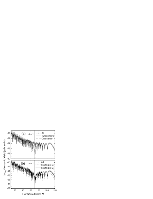
Figure 5: Contributions from different types of orbits to the high-harmonic yield, for the same parameters as in Fig. 4. Panel (a) gives the contributions from the topologically similar scattering scenarios, i. e., $|M_{11}+M_{22}|^{2}$, and $|M_{12}+M_{21}|^{2},$ and panel (b) of the orbits starting at the same center, i.e., $|M_{11}+M_{12}|^{2}$ and $|M_{21}+M_{22}|^{2}.$ All results in this figure have been computed mimicking the above-stated processes by employing the modified prefactors (27)-(30) and single-atom saddle-point equations.

The prefactor $d_{\mathrm{ion}}^{(j\nu)}$ corresponds to the transition amplitudes $M_{jj}+M_{\nu j}$ in which the electron starts at the same center and recombines with different centers in the molecule. The prefactor $d_{\mathrm{end}}^{(j\nu)}$ is related to the transition amplitudes $M_{\nu j}+M_{jj}$ in which the electron starts at different centers, but ends at the same center $C_{j}$. Finally, $d_{\mathrm{same}}$ and $d_{\mathrm{diff}}$ corresponds to the topologically similar processes, in which only one, or two center scenarios, respectively, are involved. Interestingly, only the prefactors $d_{\mathrm{ion}}^{(j\nu)}$ lead to the same interference conditions as the overall double-slit prefactor (8).

Furthermore, one should note that, if all parameters involved were real, for the first two prefactors there would be the symmetry $|d_{\mathrm{ion}}^{(j\nu)}(\mathbf{k},t,t^{\prime})|^{2}=|d_{\mathrm{ion}}^{(\nu j)}(\mathbf{k},t,t^{\prime})|^{2}$ and $|d_{\mathrm{end}}^{(j\nu)}(\mathbf{k},t,t^{\prime})|^{2}=|d_{\mathrm{end}}^{(\nu j)}(\mathbf{k},t,t^{\prime})|^{2}.$ This would lead to the same transition probabilities, as one transition amplitude is the complex conjugate of the other. This is, however, not the case, and can be seen by inspecting Eq. (III.2). Specifically in the length gauge, $\mathbf{\tilde{k}}(t^{\prime})\mathbf{=k+A}(t^{\prime})$. Depending on the center, this will lead to exponentially decreasing or increasing factors $\exp[\mp\mathrm{Im}[k+A(t^{\prime})]R]$ in the transition probability $|M_{jj}+M_{\nu j}|^{2}.$ Clearly, this procedure is less rigorous than that adopted in the previous section, as we are not considering the influence of the potential-energy shifts in the imaginary part of $t^{\prime}.$

In Fig. 5, we display the results obtained following the above-stated procedure, for the same parameters as in Fig.4. Once more, we see that the contributions of topologically similar processes, involving either one or two centers, do not lead to a well-defined interference minimum (Fig. 5.(a)). Additionally, the quantum interference of the two different kinds of processes starting from the same center $C_{j}$ leads to a well-defined minimum at the expected frequency $\Omega=69\omega$. Furthermore, the contributions from the orbits starting at $C_{2}$ are also roughly one order of magnitude smaller. The main difference between the two approaches is that the interference minimum is much deeper if modified prefactors are taken, as compared with the results obtained with modified saddle-point equations. This discrepancy is present throughout, and has also been observed in Ref. F2007 .

IV Conclusions

The results presented in this work indicate that the double-slit interference maxima and minima in the high-order harmonic spectra, which are attributed to HHG at spatially separated centers, are mainly due to the quantum interference between the processes $|M_{jj}+M_{j\nu}|^{2}$, $(j=1,2)$ in which the electron is released in the continuum at a center $C_{j}$ in the molecule, and, subsequently, recombine either at the same center or at a different center $C_{\nu}$. This can be seen either by employing modified saddle-point equations, in which the one-or two center scenarios are incorporated in the action, or by utilizing modified prefactors in which only the above-stated processes are included. In particular, when using the latter method, the transition amplitudes related to both processes can be grouped in such a way that the corresponding prefactor $d_{\mathrm{ion}}^{(j\nu)}(\mathbf{k},t,t^{\prime})$ exhibits the same interference conditions as those in the overall prefactor (8). This is in agreement with the results obtained in F2007 .

These results are not obvious, as there are other processes which lead to high-order harmonic emission at different centers in the molecule. They do not lead, however, to the double-slit interference patterns. This is due to the fact that, in the present framework, there exist potential-energy shifts that, depending on the center, sink or increase the barrier through which the electron must initially tunnel. Therefore, they strongly suppress the contributions to the spectra from one of the centers in the molecule. This will lead to an absence of the two-center interference patterns for processes starting at different centers. We have verified that this suppression occurs even for small internuclear separations.

Such potential-energy shifts, however, are only present in the length-gauge strong-field approximation and have raised a great deal of controversy PRACL2006 ; F2007 ; BCCM2007 ; SSY2007 . In fact, it is not even clear whether they are not an artifact of the SFA. On the other hand, even if single-atom saddle-point equations are taken, we found a suppression in the yield for one of the centers of the molecule. This in principle counterintuitive result is related to the fact that the electron start time $t^{\prime}$ has a non-vanishing imaginary part, which suppresses or enhances the yield through the corresponding prefactors.

- (1) See, e.g., A. Scrinzi, M. Y. Ivanov, R. Kienberger, and D. M. Villeneuve, J. Phys. B 39, R1 (2006) for a review onn the subject.
- (2) P. B. Corkum, Phys. Rev. Lett. 71, 1994 (1993); K. C. Kulander, K. J. Schafer, and J. L. Krause in: B. Piraux et al. eds., Proceedings of the SILAP conference, (Plenum, New York, 1993).
- (3) M. Lewenstein, Ph. Balcou, M. Yu. Ivanov, A. L’Huillier and P. B. Corkum, Phys. Rev. A 49, 2117 (1994).
- (4) W. Becker, S. Long, and J. K. McIver, Phys. Rev. A 41, 4112 (1990); ibid. 50, 1540 (1994); M. Lewenstein, K. C. Kulander, K. J. Schafer and Ph. Bucksbaum, Phys. Rev. A 51, 1495 (1995).
- (5) M. Lein, N. Hay, R. Velotta, J. P. Marangos, and P. L. Knight, Phys. Rev. Lett. 88, 183903 (2002); Phys. Rev. A 66, 023805 (2002); M. Spanner, O. Smirnova, P. B. Corkum and M. Y. Ivanov, J. Phys. B 37, L243 (2004).
- (6) G. Lagmago Kamta and A. D. Bandrauk, Phys. Rev. A 70, 011404 (2004); ibid. 71, 053407 (2005).
- (7) V. I. Usachenko, P. E. Pyak, and Shih-I Chu, Laser Phys. 16, 1326 (2006).
- (8) H. Hetzheim, C. Figueira de Morisson Faria, and W. Becker Phys. Rev. A 76, 023418 (2007).
- (9) D. B. Milošević, Phys. Rev. A 74, 063404 (2006).
- (10) W. Becker, J. Chen, S.G. Chen, and D. B. Milošević, Phys Rev. A 76, 033403 (2007).
- (11) M. Busuladžić, A. Gazibegović-Busuladžić, D. B. Milošević, and W. Becker, Phys. Rev. A 78, 033412 (2008); Phys. Rev. Lett. 100, 203003 (2008).
- (12) R. Kopold, W. Becker and M. Kleber, Phys. Rev. A 58, 4022 (1998).
- (13) C. C. Chirilă and M. Lein, Phys. Rev. A 73, 023410 (2006).
- (14) C. Figueira de Morisson Faria, Phys. Rev. A 76, 043407 (2007).
- (15) C. Figueira de Morisson Faria, arXiv: 0807.2763 [atom-ph]
- (16) J. Muth-Böhm, A. Becker, and F. H. M. Faisal, Phys. Rev. Lett. 85, 2280 (2000); A. Jarón-Becker, A. Becker, and F. H. M. Faisal, Phys. Rev. A 69, 023410 (2004); A. Requate, A. Becker and F. H. M. Faisal, Phys. Rev. A 73, 033406 (2006).
- (17) T. K. Kjeldsen and L. B. Madsen, Phys. Rev. A 71, 023411 (2005); Phys. Rev. Lett. 95, 073004 (2005); C. P. J. Martiny and L. B. Madsen, Phys. Rev. Lett. 97, 093001 (2006); C. B. Madsen and L. B. Madsen, Phys. Rev. A 74, 023403 (2006).
- (18) V. I. Usachenko, and S. I. Chu, Phys. Rev. A 71, 063410 (2005).
- (19) X. Zhou, X. M. Tong, Z. X. Zhao and C. D. Lin, Phys. Rev. A 71, 061801(R) (2005); ibid. 72, 033412 (2005).
- (20) C. C. Chirilă and M. Lein, J. Mod. Opt. 54, 1039 (2007).
- (21) C. Figueira de Morisson Faria, T. Shaaran, X. Liu and W. Yang, Phys. Rev. A 78, 043407 (2008).
- (22) P. Salières, B. Carré, L. LeDéroff, F. Grasbon, G. G. Paulus, H. Walther, R. Kopold, W. Becker, D. B. Milošević, A. Sanpera and M. Lewenstein, Science 292, 902 (2001).
- (23) A. Fring, V. Kostrykin and R. Schrader, J. Phys. B. 29, 5651 (1996); D. Bauer, D. B. Milošević and W. Becker, Phys. Rev. A 72, 023415 (2005).
- (24) O. Smirnova, M. Spanner and M. Ivanov, J. Phys. B 39, S307 (2006).
- (25) C. Figueira de Morisson Faria, H. Schomerus and W. Becker, Phys. Rev. A 66, 043413 (2002).
- (26) O. Smirnova, M. Spanner and M. Ivanov, J. Mod. Opt. 54, 1019 (2007).