Dynamic critical behavior of model $\bm{A}$ in films: Zero-mode boundary conditions and expansion near four dimensions

Abstract

The critical dynamics of relaxational stochastic models with nonconserved $n$-component order parameter $\bm{\phi}$ and no coupling to other slow variables (“model $A$”) is investigated in film geometries for the cases of periodic and free boundary conditions. The Hamiltonian $\mathcal{H}$ governing the stationary equilibrium distribution is taken to be $O(n)$ symmetric and to involve, in the case of free boundary conditions, the boundary terms $\int_{\mathfrak{B}_{j}}\mathring{c}_{j}\,\phi^{2}/2$ associated with the two confining surface planes $\mathfrak{B}_{j}$, $j=1,2$, at $z=0$ and $z=L$. Both enhancement variables $\mathring{c}_{j}$ are presumed to be subcritical or critical, so that no long-range surface order can occur above the bulk critical temperature $T_{c,\infty}$. A field-theoretic renormalization-group study of the dynamic critical behavior at $d=4-\epsilon$ bulk dimensions is presented, with special attention paid to the cases where the classical theories involve zero modes at $T_{c,\infty}$. This applies when either both $\mathring{c}_{j}$ take the critical value $\mathring{c}_{\text{sp}}$ associated with the special surface transition or else periodic boundary conditions are imposed. Owing to the zero modes, the $\epsilon$ expansion becomes ill-defined at $T_{c,\infty}$. Analogously to the static case, the field theory can be reorganized to obtain a well-defined small-$\epsilon$ expansion involving half-integer powers of $\epsilon$, modulated by powers of $\ln\epsilon$. This is achieved through the construction of an effective ($d-1$)-dimensional action for the zero-mode component of the order parameter by integrating out its orthogonal component via renormalization-group improved perturbation theory. Explicit results for the scaling functions of temperature-dependent finite-size susceptibilities at temperatures $T\geq T_{c,\infty}$ and of layer and surface susceptibilities at the bulk critical point are given to orders $\epsilon$ and $\epsilon^{3/2}$, respectively. They show that $L$ dependent shifts of the multicritical special point occur along the temperature and enhancement axes. For the case of periodic boundary conditions, the consistency of the expansions to $O(\epsilon^{3/2})$ with exact large-$n$ results is shown. We also discuss briefly the effects of weak anisotropy, relating theories whose Hamiltonian involves a generalized square gradient term $B^{kl}\partial_{k}\bm{\phi}\cdot\partial_{l}\bm{\phi}$ to those with a conventional $(\nabla\bm{\phi})^{2}$ term.

I Introduction

The renormalization group (RG) approach has played an important role in the modern theory of critical phenomena. RGr ; Wilson and Kogut (1974); Wegner (1976); Fisher (1998) For one thing, it provides an appropriate mathematical framework for the formulation of the theory. Second, it has led to the development of powerful calculational tools for quantitatively accurate investigations. Its most impressive and numerous successes have been achieved in the study of static bulk critical phenomena. However, appropriate extensions for studies of dynamic bulk critical phenomena, Hohenberg and Halperin (1977); Folk and Moser (2006) boundary critical phenomena,Diehl (1986, 1997) and finite-size effects rem (a); Symanzik (1981); Brézin (1982); Brézin and Zinn-Justin (1985); Rudnick et al. (1985); Barber (1983); Privman (1990); Brankov et al. (2000); Zinn-Justin (2002); Goldschmidt (1987a); Niél and Zinn-Justin (1987); Diehl (1987); Dohm (1989, 1993) were developed, which have proven their utility and power. Anyone of the features, “dynamics”, “boundaries”, and “finite size,” involves fundamental new issues and adds to the technical complexity of analytic RG studies. It is therefore not surprising that work on problems involving combinations of several of these features has remained rather scarce.

In this paper we shall be concerned with the dynamics of systems in slabs $\mathbb{R}^{d-1}\times[0,L]$ of finite thickness $L$ near their bulk ($L=\infty$) critical point. Both the cases of periodic and free boundary conditions will be considered. Hence we shall have to deal with all three of the above-mentioned features.

Despite the availability of some experimental results, there exist only few previous studies of dynamic critical behavior of systems in film geometry (see Ref. Barmatz et al., 2007 and its references). In two earlier papers, Calvo and Ferrell Calvo and Ferrell (1985); Calvo (1985) investigated the dynamics of binary liquid mixtures confined between two parallel plates using the mode-mode coupling approach. Subsequently, the dynamics of bounded one-component fluids near the liquid-gas critical point (model $H$ in the terminology of Ref. Hohenberg and Halperin, 1977) and of confined liquid ⁴He at the superfluid transition (model $E$) were analyzed by this method.Bhattacharjee (1996) There exist also a number of papers dealing with finite-size effects on dynamic critical behavior and dynamic surface critical behavior. Dietrich and Diehl (1983); Diehl (1987); Goldschmidt (1987a, b); Niél and Zinn-Justin (1987); Diehl and Dietrich (1985); Frank and Dohm (1989); Xiong and Gong (1989a, b); Frank and Dohm (1991); Binder and Frisch (1991); Diehl and Ritschel (1993); Diehl and Janssen (1992); Dohm (1993); Diehl (1994); Wichmann and Diehl (1995); Ritschel and Czerner (1995); Ritschel and Diehl (1996); Krech et al. (2001); Diehl et al. (2002); Manias et al. (2007) In other works, finite-size systems with long-range interactions or quenched disorder were investigated.Chamati and Tonchev (2001); Chamati et al. (2002); Gambassi, A. (2008)

Recently, Gambassi and Dietrich Gambassi and Dietrich (2006) presented a fairly detailed study of the familiar model $A$ (Refs. Hohenberg and Halperin, 1977 and Folk and Moser, 2006) in film geometry within the framework of the classical (zero-loop, van Hove) approximation, augmented by RG-improved perturbation theory. They focused on the situation where the surface interactions on both confining surfaces are subcritically enhanced. This corresponds to the case in which ordinary surface transitions Diehl (1986); Binder (1983) occur in the semi-infinite systems bounded by either one of the two surface planes. Knowing that Dirichlet boundary conditions apply under these conditions at both boundary planes on sufficiently large length scales, they restricted their analysis by choosing such boundary conditions from the outset.

In the present paper we shall also be concerned with model $A$ in film geometry. Our analysis complements and goes beyond that of Ref. Gambassi and Dietrich, 2006 in several ways. First, we shall not limit ourselves to the classical approximation but present a RG analysis in $d=4-\epsilon$ bulk dimensions, going to one-loop order in our explicit calculations (and partly beyond to determine contributions of order $\epsilon^{3/2}$). Second, we shall give up the restriction to Dirichlet boundary conditions on both confining plates. Aside from periodic boundary conditions, we shall consider, in the general part of our analysis, the generic case of symmetry preserving Robin boundary conditions corresponding to distinct enhancements of the surface interactions on the two boundary planes. This includes the case of special-special (sp-sp) boundary conditions for which the surface interactions on both boundary planes are critically enhanced. Krech and Dietrich (1992); Diehl et al. (2006); Grüneberg and Diehl (2008)

Periodic and sp-sp boundary conditions share the feature that Landau theory involves a zero mode at bulk criticality. It has recently become clear that this causes a breakdown of the $\epsilon$ expansion at $T_{c,\infty}$. Diehl et al. (2006); Grüneberg and Diehl (2008) The small-$\epsilon$ expansions of the associated universal amplitudes of the critical Casimir forces were found to involve, besides integer powers of $\epsilon$, also fractional powers $\epsilon^{k/2}$ with $k\geq 3$ (modulo powers of $\ln\epsilon$). This breakdown of the $\epsilon$ expansion is similar to the one reported in Ref. Sachdev, 1997 for the $3-d$ expansion of bosonic quantum systems.

The primary aim of this paper is to show that a similar breakdown of the $\epsilon$ expansion is encountered in the study of dynamic critical behavior of model $A$ in film geometry for periodic and sp-sp boundary conditions. We shall demonstrate this explicitly by determining the contributions of order $\epsilon^{3/2}$ of the dynamic finite-size susceptibility $\chi_{L}$ for both boundary conditions, the layer susceptibility $\chi^{(\text{per})}_{zz}(L)$ for periodic boundary conditions, and their surface analogs $\chi^{(\text{sp-sp})}_{11}(L)$ and $\chi^{(\text{sp-sp})}_{1L}(L)$ for sp-sp boundary conditions at $T_{c,\infty}$.

The remainder of this paper is organized as follows. In Sec. II, we first define an appropriate extension of model $A$ to the film geometry. We then recall the Lagrangian formulation of the corresponding Langevin equation Janssen (1976); de Dominicis (1976); Janssen (1992); Dietrich and Diehl (1983) along with some necessary background such as the fluctuation-dissipation theorem and the boundary conditions of the order-parameter field $\bm{\phi}$ and the associated response field $\tilde{\bm{\phi}}$. Diehl and Janssen (1992); Diehl (1994) In Sec. III, we set up perturbation theory, explain the renormalization of the theory for $d=4-\epsilon$, give the RG equations of the multi-point correlation and response functions, and describe their solutions. Section IV begins with a discussion of the basis of RG-improved perturbation theory. Next, we show that the $\epsilon$ expansion breaks down at $T_{c,\infty}$ for periodic and sp-sp boundary conditions and elucidate the origin of the problem. To obtain well-defined small-$\epsilon$ expansions, we then construct an effective ($d-1$)-dimensional dynamic field theory for the zero-mode components of $\bm{\phi}$ and $\tilde{\bm{\phi}}$. In Sec. V we present one-loop results for various scaling functions for $T\geq T_{c,\infty}$. Section VI contains a brief summary and concluding remarks. In addition, we briefly embark on the issue of universality violations due to weak anisotropy and other sources brought up recently.Chen and Dohm (2002); Dohm (2008) Finally, there are three appendixes in which technical details are described.

II The model and background

II.1 Definition of model $A$ in film geometry

We begin by defining an appropriate extension of model $A$ for the film geometry. To this end, we consider a film occupying the region $\mathfrak{V}=\mathbb{R}^{d-1}\times[0,L]$ of $d$-dimensional space $\mathbb{R}^{d}$. We wish to study the critical dynamics of such films involving an $n$-component order-parameter field $\bm{\phi}(\bm{x},t)=(\phi_{\alpha}(\bm{x},t),\alpha=1,\dotsc,n)$. We write position vectors as $\bm{x}=(\bm{y},z)$, where $\bm{y}\in\mathbb{R}^{d-1}$ and $z\in[0,L]$ are the coordinates alongside and across the film, respectively. We choose periodic boundary conditions along the $d-1$ principal $y$ directions. Depending on whether we are concerned with periodic or free boundary conditions in the $z$-direction, the slab $\mathfrak{V}$ has no boundary, $\partial\mathfrak{V}=\emptyset$, or consists of the two ($d-1$)-dimensional confining hyperplanes $\mathfrak{B}_{1}$ at $z=0$ and $\mathfrak{B}_{2}$ at $z=L$. In the latter case, we orient the boundary such that the normal $\bm{n}$ on $\partial\mathfrak{V}=\mathfrak{B}\equiv\mathfrak{B}_{1}\cup\mathfrak{B}_{2}$ points in the interior of $\mathfrak{V}$.

We are interested in the dynamics of systems that relax to a stationary equilibrium state described by the Hamiltonian (in units of $k_{B}T$)

$$\mathcal{H}[\bm{\phi}] = \int_{\mathfrak{V}}d^{d}x\,\bigg{[}\frac{1}{2}\left(\nabla\bm{\phi}\right)^{2}+\frac{\mathring{\tau}}{2}\phi^{2}+\frac{\mathring{u}}{4!}\phi^{4}\bigg{]}$$ (1)

$$+\delta_{\wp,f}\sum_{j=1}^{2}\int_{\mathfrak{B}_{j}}d^{d-1}y\,\frac{\mathring{c}_{j}}{2}\,\phi^{2}\;.$$

Here the contributions localized on the boundary planes $\mathfrak{B}_{j}$, given in the second line of Eq. (1), are only present for free boundary conditions ($\wp=f$) but absent for periodic boundary conditions ($\wp=\mathrm{per}$). The absence of boundary terms linear in $\bm{\phi}$ reflects our assumption that the boundaries do not break the $\bm{\phi}\to-\bm{\phi}$ of the Hamiltonian. That no quadratic anisotropies have been taken into account in the boundary terms meets our stronger requirement that the boundaries do not break the presumed $O(n)$ symmetry. Surface spin anisotropies, which would require separate enhancement variables $\mathring{c}_{j,\alpha}$ for the boundary terms $\propto\phi_{\alpha}^{2}$ of different components $\alpha$, Diehl and Eisenriegler (1982, 1984) will not be considered here.

For the sake of simplicity, we shall furthermore assume that the values of both surface variables $\mathring{c}_{j}$ are such that no long-range surface order can occur at $\mathfrak{B}_{j}$ above the bulk critical temperature $T_{c,\infty}$. Recall that in a semi-infinite system bounded by $\mathfrak{B}_{j}$, a transition to a bulk-disordered, surface-ordered phase takes place at a temperature $T_{c,s}>T_{c,\infty}$ when $\mathring{c}_{j}$ drops below the threshold value $\mathring{c}_{\mathrm{sp}}$ associated with the so-called special transition (provided the dimension $d$ is sufficiently large that the $d-1$ dimensional surface can support long-range order). Thus, our assumption translates into the conditions

$$\delta\mathring{c}_{j}\equiv\mathring{c}_{j}-\mathring{c}_{\mathrm{sp}}\geq 0\;,\quad j=1,2\;;$$ (2)

their physical meaning is that the surface pair interactions are subcritically ($\delta\mathring{c}_{j}>0$) or critically ($\delta\mathring{c}_{j}=0$) but not supercritically ($\delta\mathring{c}_{j}<0$) enhanced.

We are now ready to define an appropriate extension of model $A$ to the film geometry considered that is compatible with our assumptions. Straightforward considerations analogous to those made in Refs. Diehl and Janssen, 1992 and Diehl, 1994 for semi-infinite systems lead us to consider the Langevin equations

$$\dot{\phi}_{\alpha}(\bm{x},t)=-\mathring{\lambda}\,\frac{\delta\mathcal{H}}{\delta\phi_{\alpha}}(\bm{x},t)+\zeta_{\alpha}(\bm{x},t)\;,$$ (3a)

which are meant in the sense of Ito.van Kampen (1992) Here $$\mathring{\lambda} \bm{\zeta}$$ is the bare Onsager coefficient and is a Gaussian random force of mean zero,

$$\langle\zeta_{\alpha}(\bm{x},t)\rangle=0\;,$$ (3b)

and variance

$$\langle\zeta_{\alpha}(\bm{x},t)\,\zeta_{\alpha^{\prime}}(\bm{x}^{\prime},t^{\prime})\rangle=2\mathring{\lambda}\,\delta_{\alpha\alpha^{\prime}}\,\delta(\bm{x}-\bm{x}^{\prime})\,\delta(t-t^{\prime})\;.$$ (3c)

II.2 Lagrangian formulation of the theory

In our subsequent analysis of this model it will be convenient to use its equivalent Lagrangian formulation. Janssen (1976); de Dominicis (1976); Janssen (1992); Dietrich and Diehl (1983); Diehl and Janssen (1992); Diehl (1994) This involves the action

$$\mathcal{J}[\tilde{\bm{\phi}},\bm{\phi}] = \int_{t_{i}}^{t_{f}}\!dt\,\bigg{[}\int_{\mathfrak{V}}\bigg{\{}\tilde{\bm{\phi}}\cdot\bigg{[}\mathring{\lambda}\,\bigg{(}\overleftarrow{\nabla}\cdot\overrightarrow{\nabla}+\mathring{\tau}+\frac{\mathring{u}}{3!}\,\phi^{2}\bigg{)}\bm{\phi}$$ (4)

$$+\dot{\bm{\phi}}-\mathring{\lambda}\,\tilde{\bm{\phi}}\bigg{]}\bigg{\}}+\delta_{\wp,f}\mathring{\lambda}\sum_{j=1}^{2}\int_{\mathfrak{B}_{j}}\,\mathring{c}_{j}\,\tilde{\bm{\phi}}\cdot\bm{\phi}\bigg{]},\phantom{(2.4)}$$

where $\tilde{\bm{\phi}}$ is an auxiliary field, the so-called response field. The gradient operators $\overleftarrow{\nabla}$ and $\overrightarrow{\nabla}$ act as indicated to the left and right, respectively.Diehl and Janssen (1992); Diehl (1994); rem (b) Note that we have dropped a contribution $\propto\theta(t=0)$ [where $\theta(t)$ is the Heaviside function] produced by the Jacobian $\det(\delta\zeta_{\alpha}/\delta\phi_{\beta})$, choosing a prepoint discretization in time.

We fix the initial condition for the solutions to Eq. (3) in the infinite past, taking the limits $t_{i}\to-\infty$ and $t_{f}\to\infty$, and suppress these integration limits henceforth. Multipoint correlation functions of the fields $\phi_{\alpha}(\bm{x},t)$ and $\tilde{\phi}_{\tilde{\alpha}}(\tilde{\bm{x}},\tilde{t})$ can then be calculated with the functional weight $\exp(-\mathcal{J}[\tilde{\bm{\phi}},\bm{\phi}])\,\mathcal{D}[\tilde{\bm{\phi}},\bm{\phi}]$, where the measure $\mathcal{D}[\tilde{\bm{\phi}},\bm{\phi}]$ is proportional to $\prod_{\bm{x},\alpha,t}d(\tilde{\phi}_{\alpha}/2\pi i)\,d\phi_{\alpha}$ and normalized such that

$$\int\mathcal{D}[\tilde{\bm{\phi}},\bm{\phi}]\,e^{-\mathcal{J}[\tilde{\bm{\phi}},\bm{\phi}]}=1\;.$$ (5)

The field $\tilde{\phi}_{\alpha}(\bm{x},t)$ describes how averages $\langle\mathcal{O}[\bm{\phi}]\rangle$ of observables $\mathcal{O}[\bm{\phi}]$ obtained from the solutions to the Langevin equation (3) upon averaging over noise histories respond to perturbations that change its right-hand side by a function $\tilde{J}_{\alpha}(\bm{x},t)$. In the case of model $A$, the addition of the time-dependent magnetic-field terms

$$\mathcal{H}_{\text{fields}} = -\int_{\mathfrak{V}}d^{d}x\,\mathring{\bm{h}}(\bm{x},t)\cdot\bm{\phi}(\bm{x},t)$$ (6)

$$-\delta_{\wp,f}\int_{\mathfrak{B}}d^{d-1}y\,\mathring{\bm{h}}^{\mathfrak{B}}(\bm{x},t)\cdot\bm{\phi}(\bm{x},t)$$

to Hamiltonian (1) would yield such a perturbation with $\tilde{J}_{\alpha}(\bm{x},t)=\mathring{\lambda}\,h_{\alpha}(\bm{x},t)$ for $\bm{x}\notin\mathfrak{B}$ and corresponding boundary terms $\propto h_{\alpha}^{\mathfrak{B}}$. To explain the consequences, let us introduce the generating functional

$$\mathcal{G}[\tilde{\bm{J}},\tilde{\bm{K}};\bm{J},\bm{K}] = \ln\bigg{\langle}\exp\bigg{\{}\int dt\,\bigg{[}\int_{\mathfrak{V}}\big{(}\tilde{\bm{J}}\cdot\tilde{\bm{\phi}}+\bm{J}\cdot\bm{\phi}\big{)}$$ (7)

$$+\int_{\mathfrak{B}}\big{(}\tilde{\bm{K}}\cdot\tilde{\bm{\phi}}+\bm{K}\cdot\bm{\phi}\big{)}\bigg{]}\bigg{\}}\bigg{\rangle}\;,$$

where $\tilde{\bm{K}}$ and $\bm{K}$ are source functions localized on the boundary $\mathfrak{B}$. They serve to generate the boundary operators $\tilde{\bm{\phi}}^{\mathfrak{B}}=\tilde{\bm{\phi}}(\bm{x}_{\mathfrak{B}},t)$ and $\bm{\phi}^{\mathfrak{B}}=\bm{\phi}(\bm{x}_{\mathfrak{B}},t)$ with $\bm{x}_{\mathfrak{B}}\in\mathfrak{B}$ by functional differentiation. In the case of periodic boundary conditions, they are not needed, and we write $\mathcal{G}[\tilde{\bm{J}};\bm{J}]$ for the analog of functional (7).

To specify a boundary point $\bm{x}_{\mathfrak{B}}$, we must say on which boundary plane $\mathfrak{B}_{j}$ it is located and give its lateral coordinate $\bm{r}$. Denoting the restriction of $\phi_{\alpha}$f to $\mathfrak{B}_{j}$ by $\phi_{\alpha}^{\mathfrak{B}_{j}}$, we can write the boundary operators as $\phi_{\alpha}^{\mathfrak{B}_{j}}(\bm{r},t)$ and $\tilde{\phi}_{\alpha}^{\mathfrak{B}_{j}}(\bm{r},t)$. Whenever we do not wish to specify on which surface plane these boundary operators are localized, we continue writing $\phi_{\alpha}^{\mathfrak{B}}$ and $\tilde{\phi}_{\alpha}^{\mathfrak{B}}$. Analogous conventions will be used for the boundary sources $\tilde{K}^{\mathfrak{B}_{j}}_{\alpha}$ and $K^{\mathfrak{B}_{j}}_{\alpha}$ and the boundary magnetic fields $\mathring{h}_{\alpha}^{\mathfrak{B}_{j}}$.

Functional (7) generates the cumulants

$$\left\langle\prod_{i=1}^{\tilde{N}}\tilde{\phi}_{\tilde{\alpha}_{i}}\prod_{k=1}^{\tilde{M}}\tilde{\phi}_{\tilde{\beta}_{k}}^{\mathfrak{B}}\prod_{l=1}^{N}\phi_{\alpha_{l}}\prod_{m=1}^{M}\phi_{\beta_{m}}^{\mathfrak{B}}\right\rangle^{\text{cum}}$$ (8)

$$\equiv \mathring{\lambda}^{-\tilde{N}-\tilde{M}}\,W^{(\tilde{N},\tilde{M};N,M)}$$

whose $\tilde{N}+N+\tilde{M}+M$ position vectors, time arguments, and tensorial indices we have suppressed. From the correspondences

$$\frac{\mathring{\lambda}\,\delta}{\delta\tilde{J}_{\alpha}(\bm{x},t)}\leftrightarrow\frac{\delta}{\delta\mathring{h}_{\alpha}(\bm{x},t)}\leftrightarrow\mathring{\lambda}\,\tilde{\phi}_{\alpha}(\bm{x},t)$$ (9)

and

$$\frac{\mathring{\lambda}\,\delta}{\delta\tilde{K}^{\mathfrak{B}_{j}}_{\alpha}(\bm{r},t)}\leftrightarrow\frac{\delta}{\delta\mathring{h}^{\mathfrak{B}_{j}}_{\alpha}(\bm{r},t)}\leftrightarrow\mathring{\lambda}\,\tilde{\phi}^{\mathfrak{B}_{j}}_{\alpha}(\bm{r},t)$$ (10)

it is clear that the functions $W^{(\tilde{N},\tilde{M};N,M)}$ defined in Eq. (8) are the usual connected correlation and response functions.

II.3 Fluctuation-dissipation theorem and mesoscopic boundary conditions

Several other remarks are in order here, which concern the fluctuation-dissipation theorem and the boundary conditions on the mesoscopic scale where our continuum approximation applies.

First, the fluctuation-dissipation theoremHohenberg and Halperin (1977)

$$\mathring{\lambda}\,\langle\phi_{\alpha}(\bm{x},t)\,\tilde{\phi}_{\alpha^{\prime}}(\bm{x}^{\prime},t^{\prime})\rangle$$ (11)

$$= -\theta(t-t^{\prime})\,\partial_{t}\langle\phi_{\alpha}(\bm{x},t)\,\phi_{\alpha^{\prime}}(\bm{x}^{\prime},t^{\prime})\rangle^{\text{cum}}$$

holds. Second, the boundary contributions to the classical equations of motions yield the boundary conditions

$$\partial_{n}\tilde{\bm{\phi}}(\bm{x},t) = \mathring{c}_{j}\,\tilde{\bm{\phi}}(\bm{x},t)\,,\;\;\bm{x}\in\mathfrak{B}_{j}\,,$$

$$\partial_{n}\bm{\phi}(\bm{x},t) = \mathring{c}_{j}\,\bm{\phi}(\bm{x},t)\,,\;\;\bm{x}\in\mathfrak{B}_{j}\,.$$ (12)

These hold beyond the classical approximation inside of averages (up to anomalies at coinciding points).Diehl and Janssen (1992); Diehl (1994); Wichmann and Diehl (1995) On the level of the classical (zero-loop) approximation, they ensure that the matrix integral kernel

$$\bm{\mathcal{J}}^{(2)}\equiv\begin{pmatrix}2\mathring{\lambda}&\partial_{t}+\mathring{\lambda}(-\triangle+\mathring{\tau})\\ -\partial_{t}+\mathring{\lambda}(-\triangle+\mathring{\tau})&0\end{pmatrix}\otimes(\delta_{\alpha\beta})$$ (13)

of the quadratic part of $\mathcal{J}[\tilde{\bm{\phi}},\bm{\phi}]$ is self-adjoint. Third, the boundary conditions (12) imply that the fluctuation-dissipation theorem (11) remains valid when either $\bm{x}$ or $\bm{x}^{\prime}$ approaches a surface point.

In the case of periodic boundary conditions, we have

$$\tilde{\bm{\phi}}(\bm{x}+L\bm{e}_{z},t) = \tilde{\bm{\phi}}(\bm{x},t)\,,$$

$$\bm{\phi}(\bm{x}+L\bm{e}_{z},t) = \bm{\phi}(\bm{x},t)\,,$$ (14)

instead of Eq. (12).

III Perturbation theory and RG

III.1 Free propagators

To set up perturbation theory, we employ dimensional regularization and focus on the disordered phase. The free response and correlation propagators, $R_{L}$ and $C_{L}$, then follow from the inverse of the matrix kernel (13). We have

$$\Big{[}\bm{\mathcal{J}}^{(2)}\Big{]}^{-1}\equiv\bm{G}_{L}=\begin{pmatrix}0&R_{L}^{\dagger}\\ R_{L}&C_{L}\end{pmatrix}\otimes(\delta_{\alpha\beta})\;.$$ (15)

where $R_{L}$ is the solution to

$$\big{[}\partial_{t}+\mathring{\lambda}(-\triangle+\mathring{\tau})\big{]}\,R_{L}(\bm{x},t;\bm{x}^{\prime},t^{\prime})=\delta(\bm{x}-\bm{x}^{\prime})\,\delta(t-t^{\prime})\,,$$ (16)

while $C_{L}$ is proportional to the convolution $R_{L}\ast R_{L}^{\dagger}$:

$$C_{L}(\bm{x},t;\bm{x}^{\prime},t^{\prime})=2\mathring{\lambda}\,(R_{L}\ast R_{L}^{\dagger})(\bm{x},t;\bm{x}^{\prime},t^{\prime})$$ (17)

$$= 2\mathring{\lambda}\int_{-\infty}^{\infty}d\tilde{t}\int_{\mathfrak{V}}d^{d}\tilde{x}\,R_{L}(\bm{x},t;\tilde{\bm{x}},\tilde{t})\,R_{L}(\tilde{\bm{x}},\tilde{t};\bm{x}^{\prime},t^{\prime})\,.\quad$$

The $\bm{y}t$-Fourier transforms of these quantities (for which we use the notational conventions summarized in Appendix A) can be expressed as

$$R_{L}(\bm{p};z,z^{\prime};\omega)=\sum_{m}\frac{f_{m}(z)\,f^{*}_{m}(z^{\prime})}{-i\omega+\mathring{\lambda}\,(\mathring{\tau}+p^{2}+k_{m}^{2})}$$ (18)

and

$$C_{L}(\bm{p};z,z^{\prime};\omega)=\sum_{m}\frac{2\mathring{\lambda}\,f_{m}(z)\,f^{*}_{m}(z^{\prime})}{\big{|}-i\omega+\mathring{\lambda}\,(\mathring{\tau}+p^{2}+k_{m}^{2})\big{|}^{2}}\phantom{(2.19}$$ (19)

in terms of a complete set of orthonormal eigenfunctions $f_{m}(z)$ of the operator $-\partial_{z}^{2}$, where $f_{m}^{*}(z^{\prime})$ is the complex conjugate of $f_{m}(z^{\prime})$. These functions are properly normalized solutions to

$$-\partial_{z}^{2}\,f_{m}(z)=k_{m}^{2}\,f_{m}(z)\;,$$ (20)

subject to the boundary conditions

$$f_{m}^{\prime}(0) = \mathring{c}_{1}\,f_{m}(0)\;,$$

$$-f_{m}^{\prime}(L) = \mathring{c}_{2}\,f_{m}(L)\;.$$ (21)

For non-negative values of $\mathring{c}_{1}$ and $\mathring{c}_{2}$, the spectrum $\{k^{2}_{m}\}$ is discrete with $k_{m}^{2}\geq 0$. The eigenfunctions are phase-shifted cosine functions $f_{m}(z)=A_{m}\cos(k_{m}z+\vartheta_{m})$, whose phase shift $\vartheta_{m}$ follows from the first of the boundary conditions (III.1). The eigenvalues are solutions to the transcendental equation implied by the boundary condition at $z=L$. For general values of $\mathring{c}_{j}\geq 0$, the eigenvalues $k_{m}^{2}$ depend on both $\mathring{c}_{1}$ and $\mathring{c}_{2}$, as do the normalization factors $A_{m}$ and the phase shifts $\vartheta_{m}$ (via $k_{m}$).Romeo and Saharian (2002); Schmidt (2008); Schmidt and Diehl (2008) For the special values $(\mathring{c}_{1},\mathring{c}_{2})=(\infty,\infty)$, $(0,0)$, and $(\infty,0)$ corresponding to the combinations D-D, N-N, and D-N of Dirichlet (D) and Neumann (N) boundary conditions on the two planes, the eigenvalues $k_{m}^{2}$ and eigenfunctions $f_{m}$ can be found in Appendix A of Ref. Krech and Dietrich, 1992 and Appendix A of Ref. Krech, 1994.

However, the response propagator $R_{L}(\bm{p};z,z^{\prime};\omega)$ can also be determined by solving the analog of Eq. (16) in the $\bm{p}z\omega$ representation using familiar methods for Sturm-Liouville differential equations.Courant and Hilbert (1968) We give the result of such a calculation for general non-negative values of $\mathring{c}_{1}$, $\mathring{c}_{2}$, and $\mathring{\tau}$ in Eq. (133) of Appendix B. In the special cases $\mathring{c}_{1}=\mathring{c}_{2}=0$ and $\mathring{c}_{1}=\mathring{c}_{2}=\infty$, the result is equivalent to the representationsSymanzik (1981); Diehl (1986); Gambassi and Dietrich (2006)

$$R_{L}^{(\begin{subarray}{c}\text{N-N}\\ \text{D-D}\end{subarray})}(\bm{p};z_{1},z_{2};\omega) = \sum_{m=-\infty}^{\infty}\big{[}R_{\infty}(\bm{p},z_{1}-z_{2}-m2L,\omega)$$ (22)

$$\pm R_{\infty}(\bm{p},z_{1}+z_{2}-m2L,\omega)\big{]}$$

of the corresponding Neumann and Dirichlet propagators $R_{L}^{(\text{N-N})}$ and $R_{L}^{(\text{D-D})}$ as a sum of image contributions involving the bulk propagator (see, e.g., Refs. Diehl, 1986, Symanzik, 1981, and Grüneberg and Diehl, 2008)

$$R_{\infty}(\bm{p},z_{12},\omega)=\frac{1}{2\mathring{\lambda}\,\mathring{\kappa}_{\omega}}\,e^{-\mathring{\kappa}_{\omega}\,|z_{12}|}\;,$$ (23)

where $z_{12}\equiv z_{1}-z_{2}$ and

$$\mathring{\kappa}_{\omega}=\sqrt{p^{2}+\mathring{\tau}-i\omega/\mathring{\lambda}}\;.$$ (24)

In the case of periodic boundary conditions, one has

$$R_{L}^{(\text{per})}(\bm{p};z_{1},z_{2};\omega)=\sum_{m=-\infty}^{\infty}R_{\infty}(\bm{p},z_{12}-mL,\omega)\,.\;\;\;$$ (25)

The corresponding finite-size correlation propagators $C_{L}^{(\text{N-N})}$, $C_{L}^{(\text{D-D})}$, and $C_{L}^{(\text{per})}$ can be expressed in terms of the free bulk correlation propagator $C_{\infty}(\bm{p},z_{12},\omega)$ in a manner completely analogous to Eqs. (22) and (25).

III.2 Reparametrizations

As is well known and explained elsewhere,Symanzik (1981); Dietrich and Diehl (1983); Diehl (1986, 1987); Diehl and Janssen (1992); Diehl (1994) the singularities of $R_{\infty}(\bm{x}_{12},t_{12})$ and $C_{\infty}(\bm{x}_{12},t_{12})$ at coinciding points $(\bm{x}_{12},t_{12})=(\bm{0},0)$ produce ultraviolet (uv) singularities in Feynman integrals of the multipoint cumulant and response functions (8). For dimensions $d\leq 4$ and periodic boundary conditions, the uv singularities of these functions can be absorbed via standard “bulk” reparametrizations of the form

$$\bm{\phi} = Z_{\phi}^{1/2}\,\bm{\phi}_{R},$$ (26a)

$$\tilde{\bm{\phi}} = Z_{\tilde{\phi}}^{1/2}\,\tilde{\bm{\phi}}_{R},$$ (26b)

$$\mathring{\lambda} = \mu^{-2}\,[Z_{\phi}/Z_{\tilde{\phi}}]^{1/2}\lambda,$$ (26c)

$$\delta\mathring{\tau}\equiv\mathring{\tau}-\mathring{\tau}_{c} = \mu^{2}\,Z_{\tau}\tau,$$ (26d)

$$\mathring{u}\,N_{d} = \mu^{\epsilon}Z_{u}u.$$ (26e)

Here $$\mu \mathring{\tau}_{c} \mathring{\tau} d u$$ is an arbitrary momentum scale and denotes the critical value of of the -dimensional bulk theory. Following Ref. Grüneberg and Diehl, 2008, we choose the factor that is absorbed in the renormalized coupling constant as

$$N_{d} = \frac{2\,\Gamma(3-d/2)}{(d-2)(4\pi)^{d/2}}$$ (26f)

$$= \frac{1}{16\pi^{2}}\left[1+\frac{1-\gamma_{E}+\ln(4\pi)}{2}\,\epsilon+O(\epsilon^{2})\right],\phantom{(2.15)}$$

where $\gamma_{E}=-\Gamma^{\prime}(1)$ is Euler’s constant. If we employ dimensional regularization and fix the renormalization factors $Z_{g}$, $g=\phi,\tilde{\phi},u,\tau$, by minimal subtraction of poles in $\epsilon$, this convention ensures that the two-loop results for these functions given in equations (3.42a)–(3.42c) and (4.54) of Ref. Diehl, 1986 apply.

For free boundary conditions, additional primitive uv singularities with support on $\mathfrak{B}_{1}$ and $\mathfrak{B}_{2}$ occur. These can be absorbed through the additional (“surface”) reparametrizations

$$\delta\mathring{c}_{j} \equiv \mathring{c}_{j}-\mathring{c}_{\mathrm{sp}}=\mu Z_{c}\,c_{j},$$

$$\bm{\phi}^{\mathfrak{B}} = (Z_{\phi}\,Z_{1})^{1/2}\,[\bm{\phi}^{\mathfrak{B}}]_{R},$$

$$\tilde{\bm{\phi}}^{\mathfrak{B}} = (Z_{\tilde{\phi}}\,Z_{1})^{1/2}\,[\tilde{\bm{\phi}}^{\mathfrak{B}}]_{R},$$ (27)

known from the semi-infinite case, where $[\bm{\phi}^{\mathfrak{B}}]_{R}$ and $[\tilde{\bm{\phi}}^{\mathfrak{B}}]_{R}$ are renormalized boundary operators. Explicit two-loop expressions for the renormalization factors $Z_{1}$ and $Z_{c}$ may be found in Eqs. (3.66a) and (3.66b) of Ref. Diehl, 1986 or in Refs. Diehl and Dietrich, 1981 and Diehl and Dietrich, 1983.

III.3 RG equations and scaling

Upon introducing the renormalized functions

$$W^{(\tilde{N},\tilde{M};N,M)}_{R}$$ (28)

$$= Z_{\phi}^{-(\tilde{N}+N)/2}(Z_{\phi}Z_{1})^{-(\tilde{M}+M)/2}\,W^{(\tilde{N},\tilde{M};N,M)}\,,\phantom{3.14}$$

we can exploit the invariance of the bare functions $W^{(\tilde{N},\tilde{M};N,M)}$ under changes $\mu\to\mu\ell$ in a standard fashion to obtain the RG equations

$$\bigg{[}\mathcal{D}_{\mu}+(\tilde{N}+N)\,\frac{\eta_{\phi}}{2}+(\tilde{M}+M)\,\frac{\eta_{\phi}+\eta_{1}}{2}\bigg{]}W^{(\tilde{N},\tilde{M};N,M)}_{R}=0\;.$$ (29)

Here

$$\mathcal{D}_{\mu}=\mu\partial_{\mu}+\sum_{g=u,\tau,\lambda,c_{1},c_{2}}\beta_{g}\,\partial_{g}\;.$$ (30)

The beta and exponent functions $\beta_{g}$ and $\eta_{g}$ are given by

$$\beta_{g} \equiv \mu\partial_{\mu}|_{0}g=-(d_{g}+\eta_{g})g$$ (31)

$$= \begin{cases}-(\epsilon+\eta_{u})u\,,&g=u\,,\\ -(2+\eta_{\tau})\tau\,,&g=\tau\,,\\ (2-\eta_{\lambda})\lambda\,,&g=\lambda\,,\\ -(1+\eta_{c})c_{j}\,,&g=c_{j}\,,\;j=1,2\,.\end{cases}$$

and

$$\eta_{g}\equiv\mu\partial_{\mu}|_{0}g\;,\quad g=u,\tau,\phi,\tilde{\phi},\lambda,1,c_{1},c_{2}\,,$$ (32)

respectively, where $\partial_{\mu}|_{0}$ means a derivative at fixed parameters of the bare theory. Explicit results for $\beta_{u}$ to order $u^{3}$ and for $\eta_{\phi}(u)$, $\eta_{\tau}(u)$, $\eta_{1}(u)$, and $\eta_{c}(u)\equiv\eta_{c_{j}}(u)$ to order $u^{2}$ may be looked up in Eqs. (3.75a), (3.75b), (3.76a), and (3.76b) of Ref. Diehl, 1986, respectively. The function $\eta_{\lambda}$, which can be written as $\eta_{\lambda}=(\eta_{\phi}-\eta_{\tilde{\phi}})/2$, is given to order $u^{2}$ in the first line of Eq. (III.8) of Ref. Dietrich and Diehl, 1983.

It should be obvious how the above RG equations carry over to the case of periodic boundary conditions: the RG equation for $W^{(\tilde{N};N)}_{R}$ agrees with Eq. (29) if we set $\tilde{M}=M=0$, except that the contributions to $\mathcal{D}_{\mu}$ involving $\partial_{c_{j}}$ drop out because these variables do not occur in the theory when periodic boundary conditions are chosen.

Using characteristics the RG equations (29) can be exploited in a familiar fashion to derive the asymptotic scaling behavior of the functions $W^{(\tilde{N},\tilde{M};N,M)}_{R}$. Let $\bar{g}(\ell)$ be solutions to the flow equations

$$\ell\,\frac{d\bar{g}(\ell)}{d\ell}=\beta_{g}[\bar{u}(\ell),\bar{g}(\ell)]\,,\quad g=u,\tau,\lambda,c_{1},c_{2},$$ (33)

satisfying the initial conditions $\bar{g}(1)=g$. Then we have

$$\ln\ell=\int_{u}^{\bar{u}}\frac{dv}{\beta_{u}(v)}$$ (34)

and

$$\bar{g}(\ell)=E_{g}[\bar{u}(\ell),u]\,\ell^{-(d_{g}+\eta_{g}^{*})}\,g,\quad g=\tau,\lambda,c_{1},c_{2}\,,$$ (35)

where $E_{g}(\bar{u},u)$ are the trajectory integrals

$$E_{g}(\bar{u},u)=\exp\left[-\int_{u}^{\bar{u}}dv\,\frac{\eta_{g}(v)-\eta_{g}^{*}}{\beta_{u}(v)}\right]$$ (36)

and the asterisk indicates values $\eta_{g}^{*}\equiv\eta_{g}(u^{*})$ at the nontrivial root $u^{*}=O(\epsilon)$ of $\beta_{u}(u)$.

To illustrate the consequences of the RG equations (29), let us consider the multipoint cumulants in the $\bm{x}t$-presentation. Writing $W^{(\tilde{N},\tilde{M};N,M)}_{R}\equiv W_{R}(\bm{x},t;u,\tau,c_{1},c_{2},L,\lambda,\mu)$, where $\bm{x}$ and $t$ represent all position and time variables, respectively, we note that the dimension of this function is $\lambda^{\tilde{N}+\tilde{M}}\,\mu^{d_{W}}$, with

$$d_{W}=(\tilde{N}+\tilde{M})\,\frac{d+2}{2}+(N+M)\,\frac{d-2}{2}\;.$$ (37)

Using this in conjunction with the solution to the RG equation (29), one arrives at

$$W_{R}(\bm{x},t;u,\tau,c_{1},c_{2},L,\lambda,\mu)=\lambda^{\tilde{N}+\tilde{M}}\,\mu^{d_{W}}\,\ell^{\Delta_{W}}$$ (38)

$$\times E_{W}(\ell)\,W_{R}(\mu\ell\bm{x},\bar{\lambda}\mu^{2}t;\bar{u},\bar{\tau},\bar{c}_{1},\bar{c}_{2},\mu\ell L,1,1)\,.\qquad$$

Here $\Delta_{W}$ is the scaling dimension of $W_{R}$. We use the notation $\Delta[\mathcal{O}]$ for the scaling dimension of an operator $\mathcal{O}(\bm{x},t)$. Then we have

$$\Delta[\phi] \equiv (d-2+\eta_{\phi}^{*})/2=\beta/\nu\,,$$

$$\Delta[\tilde{\phi}] \equiv 2-\eta_{\lambda}^{*}+\Delta[\phi]=\mathfrak{z}+\beta/\nu\,,$$

$$\Delta[\phi^{\mathfrak{B}}] \equiv (d-2+\eta_{\phi}^{*}+\eta_{1}^{*})/2=\beta_{1}^{\text{sp}}/\nu\,,$$

$$\Delta[\tilde{\phi}^{\mathfrak{B}}] \equiv \mathfrak{z}+\Delta[\phi^{\mathfrak{B}}]=\mathfrak{z}+\beta_{1}^{\text{sp}}/\nu\,,$$ (39)

where we have introduced the standard static bulk critical indices $\beta$ and $\nu$, the dynamic bulk critical exponent $\mathfrak{z}$, and the surface critical exponent $\beta_{1}^{\text{sp}}$ of the special transition.Diehl (1986) In terms of these quantities, the scaling dimension reads

$$\Delta_{W}=\tilde{N}\Delta[\tilde{\phi}]+N\Delta[\phi]+\tilde{M}\Delta[\tilde{\phi}^{\mathfrak{B}}]+M\Delta[\phi^{\mathfrak{B}}]\,.$$ (40)

Further, the prefactor $E_{W}(\ell)$ denotes the trajectory integral

$$E_{W}(\ell)=\exp\bigg{\{}\int_{u}^{\bar{u}(\ell)}\frac{\eta_{W}(v)-\eta_{W}^{*}}{\beta_{u}(v)}\,dv\bigg{\}}$$ (41)

with

$$\eta_{W}(u)=\frac{\tilde{N}+N}{2}\,\eta_{\phi}+\frac{\tilde{M}+M}{2}\,(\eta_{\phi}+\eta_{1})-(\tilde{N}+\tilde{M})\,\eta_{\lambda}\,.$$ (42)

It is easily checked that Eq. (38) yields scaling forms in accordance with the phenomenological theory of finite-size scaling.Barber (1983); Privman (1990) Assuming that the initial coupling constant $u$ is nonzero, we replace the running coupling constant $\bar{u}$ and the scale-dependent amplitude $E_{W}(\ell)$ by their respective long-scale limits $\bar{u}(0)=u^{*}$ and $E_{W}^{*}=E_{W}(0)$ and substitute the running variables $\bar{\tau}$, $\bar{\lambda}$, and $\bar{c}_{j}$ by their limiting forms

$$\bar{g}(\ell)\underset{\ell\to 0}{\approx}E_{g}^{*}(u)\,\ell^{-(d_{g}+\eta_{g}^{*})}\,g=\begin{cases}E_{\tau}^{*}(u)\,\ell^{-1/\nu}\,\tau,\\ E_{\lambda}^{*}(u)\,\ell^{\,\mathfrak{z}}\,\lambda,\\ E_{c}^{*}(u)\,\ell^{-\Phi/\nu}\,c_{j},\end{cases}$$ (43)

where $E_{g}^{*}(u)\equiv E_{g}(u^{*},u)$ are nonuniversal amplitudes, and we have introduced the surface crossover exponent $\Phi=\nu(1+\eta_{c}^{*})$.Diehl (1986) If we now fix the scale parameter $\ell\equiv\ell_{\tau}$ for given $\tau\neq 0$ by $\bar{\tau}(\ell_{\tau})=\text{sign}(\tau)$, then

$$\mu^{-1}\ell_{\tau}^{-1}\underset{\tau\to\pm 0}{\approx}\mu^{-1}\,\big{(}E_{\tau}^{*}|\tau|\big{)}^{-\nu}$$ (44)

agrees with the second-moment bulk correlation length

$$\xi_{\infty}^{\pm}\approx\xi^{(0)}_{\pm}\,|T/T_{c,\infty}-1|^{-\nu}\;,$$ (45)

up to a nonuniversal scale factor. We thus obtain the scaling forms

$$W_{R}(\bm{x},t;u,\tau,c_{1},c_{2},L,\lambda,\mu)\approx\lambda^{\tilde{N}+\tilde{M}}\,\mu^{d_{W}}$$ (46)

$$\times\,(\mu\xi_{\infty}^{\pm})^{-\Delta_{W}}E_{W}^{*}\,\Xi_{\pm}(\bm{x}/\xi_{\infty}^{\pm},\mathsf{t};\mathsf{c}_{1},\mathsf{c}_{2},L/\xi_{\infty}^{\pm})\phantom{(3.15)}\;,$$

in which $\mathsf{t}$ represents the set of all scaled time variables

$$\mathsf{t}=E_{\lambda}^{*}\lambda\mu^{2}t\,(\mu\xi_{\infty}^{\pm})^{-\mathfrak{z}}\,,$$ (47)

while $\mathsf{c}_{1}$ and $\mathsf{c}_{2}$ denote the scaled surface variables

$$\mathsf{c}_{j}=E_{c}^{*}c_{j}\,(\mu\xi_{\infty}^{\pm})^{\Phi}\,.$$ (48)

The scaling functions $\Xi_{\pm}$ are given by the restrictions of $W_{R}(\dotsc;\bar{u},\bar{\tau},\dotsc)$ to the hyperplanes with $\bar{u}=u^{*}$ and $\bar{\tau}=\pm 1$.

Analogous results apply for periodic boundary conditions, except that the surface scaling variables $\mathsf{c}_{1}$ and $\mathsf{c}_{2}$ are missing.

IV RG-improved perturbation theory

IV.1 Background

There exist known important cases of critical phenomena, in which the infrared (IR) singularities one is concerned with originate from the divergence of a single length, such as the bulk correlation length $\xi_{\infty}$. The most familiar example is static critical behavior that occurs at a usual bulk critical point when it is approached from the disordered phase. The crux of RG-improved perturbation theory is to exploit the RG to relate the behavior of systems with large $\xi_{\infty}$ to that of systems with $\xi_{\infty}$ of order unity and then determine properties of the latter by means of appropriate perturbation theory techniques. Provided no other sources of IR singularities exist, the resulting perturbation expansions will not be plagued by problems even though sophisticated resummation methods may well be required to obtain reliable results.Zinn-Justin (2002)

In order to determine the behavior of properties at the critical point, information about the behavior of the static bulk analogs of the above scaling functions $\Xi_{\pm}$ in the limit $\bm{x}/\xi_{\infty}\to\bm{0}$ is required. In the simple case considered so far, this can be inferred from the requirement that a temperature independent nonzero limit results for the property considered. Furthermore, the form of corrections to the leading asymptotic behavior of the pair correlation function for $|\bm{x}|/\xi_{\infty}\ll 1$ can be determined via the short-distance expansion (see, e.g., Refs. Fisher and Aharony, 1974, Amit and Martin-Mayor, 2005, and their references).

However, even in the case of static bulk critical behavior, additional sources of IR singularities may exist. For example, in systems exhibiting spontaneous breakdown of continuous symmetries, IR singularities associated with Goldstone modes appear on the coexistence curve.Schäfer and Horner (1978) Other examples are provided by crossover phenomena such as the crossover away from a bicritical point. Here the crossover from one type of critical behavior to another leads to singularities in the corresponding crossover scaling functions.Amit and Goldschmidt (1978); Amit and Martin-Mayor (2005) To ensure that these IR singularities are properly taken into account in RG-improved perturbation theory is a nontrivial task. For some cases, specially designed RG schemes exists that allow one to correctly build in the asymptotic behavior at the stable fixed point to which the crossover occurs.Fisher and Aharony (1974); Lawrie (1981) Within the framework of dimensionality expansions, this usually works when the additional IR singularities are properly handled by simple theories such as the random phase approximationSchäfer and Horner (1978); Lawrie (1981) or are accessible to an $\epsilon=d^{*}-d$ expansion about the same upper critical dimension $d^{*}$.Amit and Goldschmidt (1978); Amit and Martin-Mayor (2005) Much more challenging are problems involving two distinct kinds of nontrivial critical behavior with different upper critical dimensions.

Unfortunately, the study of critical behavior in films of finite thickness belongs to the latter class of hard problems. The reason is that a full treatment would involve a proper analysis of dimensional crossover. Suppose the film undergoes for finite $L$ and given bulk dimension $d$ a sharp phase transition at a temperature $T_{c,L}$. If all interactions are ferromagnetic, this temperature must satisfy $T_{c,L}\leq T_{\infty}$ by Griffiths-Kelly-Sherman inequalities.Griffiths (1968); Kelly and Sherman (1968) On lowering the temperature from an initial temperature $T>T_{c,\infty}$, one will therefore first observe $d$-dimensional critical behavior as $L,\xi_{\infty}\to\infty$ with $L/\xi_{\infty}\gg 1$, which will cross over to $(d-1)$-dimensional critical behavior as the length $\xi_{\|}$ on which correlations along the film decay becomes much larger than $L$. Barber (1983) Since $d$- and $(d-1)$-dimensional critical behaviors involve different upper critical dimensions ($d^{*}=4$ and $d^{*}=5$, respectively), one cannot handle both of them by the same dimensionality expansion. In those cases where no sharp phase transition is possible for finite $L$, a rounded transition will occur at $T_{c,L}$. Even then, the $\epsilon$ expansion must not be expected to correctly capture the behavior for $T\simeq T_{c,L}$. Because of these and technical difficulties, previous investigations of static finite-size effects in films based on the $\epsilon$ expansionKrech and Dietrich (1992, 1991); Krech et al. (1995); fbk ; Krech (1994); Diehl et al. (2006); Grüneberg and Diehl (2008) have focused on the case $T\geq T_{c,\infty}$, even though RG-improved mean-field results for $T<T_{c}$ exist for ($d=3$)-dimensional systems with bulk critical and tricritical points.Zandi et al. (2007); Maciołek et al. (2007); rem (c); Garcia and Chan (1999); Hucht (2007); Vasilyev et al. (2007)

For simplicity, we shall restrict ourselves here also to the case $T\geq T_{c,\infty}$. We begin with a discussion of the breakdown of the $\epsilon$ expansion at $T_{c,\infty}$ for periodic and sp-sp boundary conditions. Since the latter is the only case of free boundary conditions explicitly considered henceforth, we shall no longer keep track of the enhancement variables, fixing $c_{1}$ and $c_{2}$ at zero whenever we deal with this boundary condition.

IV.2 Breakdown of $\bm{\epsilon}$ expansion at $\bm{T_{c,\infty}}$ and construction of effective action

We shall use dimensional regularization. In a perturbative approach, the critical values $\mathring{\tau}_{c}$ and $\mathring{c}_{\text{sp}}$ then vanish.Diehl and Dietrich (1981, 1983); Diehl (1986) In any case, the response and correlation propagators for sp-sp boundary conditions satisfy Neumann boundary conditions on both planes ($\wp=\text{N-N}$) at zero-loop order.

The eigenvalues $k_{m}^{2}$ of $-\partial_{z}^{2}$ for periodic ($\wp=\text{per}$) and N-N boundary conditions are given by $k^{(\mathrm{per})}_{m}=2\pi m/L$ with $m\in\mathbb{Z}$ and $k^{(\mathrm{N-N})}_{m}=\pi m/L$ with $m=0,1,\dotsc,\infty$, respectively.Krech and Dietrich (1992) In both cases, one has the eigenvalue $k_{0}^{2}=0$. As can be seen from the mode decompositions (18) and (19), the associated $k_{0}=0$ modes give IR singular contributions to the free propagators $R_{L}$ and $C_{L}$ at the bulk critical temperature ($\mathring{\tau}=0$) when $\omega=p=0$. This is an artifact of the zero-loop approximation, which predicts that a sharp phase transition occurs for finite $L$ precisely at $T_{c,\infty}$, yielding no shift $T_{c,L}-T_{c,\infty}$. For bulk and semi-infinite systems the contributions from these zero modes are negligible. However, for films of finite thickness $L$, we must be more careful.

It is known from Refs. Diehl et al., 2006 and Grüneberg and Diehl, 2008 that beyond zero-loop order, the ${k=0}$ component of the order parameter becomes critical at the shifted values $\delta\mathring{\tau}=-\delta\mathring{\tau}_{L}^{(\text{per})}$, and $-\delta\mathring{\tau}_{L}^{(\text{sp-sp})}$ given by

$$\delta\mathring{\tau}_{L}^{(\mathrm{per})}=2^{2-\epsilon}\,\delta\mathring{\tau}_{L}^{\text{(sp-sp)}}=\mathring{u}\,\frac{n+2}{6}\,\frac{\Gamma(1-\epsilon/2)\,\zeta(2-\epsilon)}{2\pi^{2-\epsilon/2}\,L^{2-\epsilon}}\,,$$ (49)

where $\zeta(s)$ denotes Riemann’s zeta function. In order to obtain a well-defined RG-improved perturbation theory at $T_{c,\infty}$, we generalize the approach of Refs. Diehl et al., 2006 and Grüneberg and Diehl, 2008 to dynamics. Writing

$$\bm{\phi}(\bm{y},z,t) = L^{-1/2}\,\bm{\varphi}(\bm{y},t)+\bm{\psi}(\bm{y},z,t)$$

$$\tilde{\bm{\phi}}(\bm{y},z,t) = L^{-1/2}\,\tilde{\bm{\varphi}}(\bm{y},t)+\tilde{\bm{\psi}}(\bm{y},z,t)$$ (50)

with

$$\int_{0}^{L}\bm{\psi}(\bm{y},z,t)\,dz=\int_{0}^{L}\tilde{\bm{\psi}}(\bm{y},z,t)\,dz=\bm{0}\,,$$ (51)

we split the fields $\bm{\phi}(\bm{x},t)$ and $\tilde{\bm{\phi}}(\bm{x},t)$ into their zero-mode components $\bm{\varphi}(\bm{y},t)$ and $\tilde{\bm{\varphi}}(\bm{y},t)$ and their $k\neq 0$ orthogonal complements $\bm{\psi}(\bm{x},t)$ and $\tilde{\bm{\psi}}(\bm{x},t)$. Upon integrating out the latter fields, we define an effective action $\mathcal{J}_{\text{eff}}[\tilde{\bm{\varphi}},\bm{\varphi}]$ for the zero-mode components by

$$\mathcal{J}_{\text{eff}}[\tilde{\bm{\varphi}},\bm{\varphi}] \equiv -\ln\text{Tr}_{\tilde{\bm{\psi}},\bm{\psi}}\,e^{-\mathcal{J}[\tilde{\bm{\psi}}+L^{-1/2}\tilde{\bm{\varphi}},\bm{\psi}+L^{-1/2}\bm{\varphi}]}$$ (52)

$$= \mathcal{J}^{[0]}_{\text{eff}}[\tilde{\bm{\varphi}},\bm{\varphi}\big{]}-\ln\left\langle e^{-\mathcal{J}_{\text{int}}[\tilde{\bm{\varphi}},\tilde{\bm{\psi}},\bm{\varphi},\bm{\psi}]}\right\rangle_{\tilde{\bm{\psi}},\bm{\psi}}\,.\quad$$

where

$$\langle\centerdot\rangle_{\tilde{\bm{\psi}},\bm{\psi}}=\int\centerdot\;e^{-\mathcal{J}[\tilde{\bm{\psi}},\bm{\psi}]}\,\mathcal{D}[\tilde{\bm{\psi}},\bm{\psi}]\,.$$ (53)

Here

$$\mathcal{J}^{[0]}_{\text{eff}}[\tilde{\bm{\varphi}},\bm{\varphi}] = \mathcal{J}\big{[}L^{-1/2}\tilde{\bm{\varphi}},L^{-1/2}\bm{\varphi}]$$ (54)

$$= \int dt\int d^{d-1}y\bigg{\{}\tilde{\bm{\varphi}}\cdot\bigg{[}\mathring{\lambda}\,\bigg{(}\mathring{\tau}-\nabla_{\bm{y}}^{2}$$

$$+\frac{\mathring{u}}{6L}\,\varphi^{2}\bigg{)}\bm{\varphi}+\dot{\bm{\varphi}}-\mathring{\lambda}\,\tilde{\bm{\varphi}}\bigg{]}\bigg{\}}$$

is the zero-loop contribution to $\mathcal{J}_{\text{eff}}[\tilde{\bm{\varphi}},\bm{\varphi}]$. The interaction part $\mathcal{J}_{\text{int}}$ is given by

$$\mathcal{J}_{\text{int}}[\tilde{\bm{\varphi}},\tilde{\bm{\psi}},\bm{\varphi},\bm{\psi}]$$ (55)

$$= \frac{\mathring{\lambda}\mathring{u}}{6L}\int dt\int_{\mathfrak{V}}\Big{[}\psi^{2}\,(\tilde{\bm{\varphi}}\cdot\bm{\varphi})+2(\tilde{\bm{\varphi}}\cdot\bm{\psi})(\bm{\varphi}\cdot\bm{\psi})$$

$$+\varphi^{2}\,(\tilde{\bm{\psi}}\cdot\bm{\psi})+2(\tilde{\bm{\psi}}\cdot\bm{\varphi})(\bm{\varphi}\cdot\bm{\psi})$$

$$+L^{-1/2}(\tilde{\bm{\psi}}\cdot\bm{\varphi})\,\psi^{2}+L^{-1/2}(\tilde{\bm{\varphi}}\cdot\bm{\psi})\,\psi^{2}\Big{]}.$$

Computing $\mathcal{J}_{\text{eff}}$ in a loop expansion and writing

$$\mathcal{J}_{\text{eff}}[\tilde{\bm{\varphi}},\bm{\varphi}]=\mathcal{J}^{[0]}_{\text{eff}}[\tilde{\bm{\varphi}},\bm{\varphi}]+\mathcal{J}_{\text{eff}}^{[1]}[\tilde{\bm{\varphi}},\bm{\varphi}]+\dotso\,,$$ (56)

one easily derives the one-loop contribution

$$\mathcal{J}_{\mathrm{eff}}^{[1]}[\tilde{\bm{\varphi}},\bm{\varphi}] = \frac{1}{2}\,\mathrm{Tr}\ln\Big{[}\openone+\frac{\mathring{\lambda}\mathring{u}}{L}\,\bm{G}^{(\wp)}_{L,\psi}\cdot\bm{B}\Big{]}$$ (57)

(cf. Ref. Diehl, 1987), where $\bm{G}^{(\wp)}_{L,\psi}$ denotes the free propagator in the $k\neq 0$ subspace for the respective boundary conditions $\wp=\text{per}$ and sp-sp. Let $P_{0}\equiv|k_{0}\rangle\langle k_{0}|$ be the projector onto this $k=0$ space and $Q_{0}=\openone-P_{0}$. Then we may write

$$\bm{G}_{L,\psi}=Q_{0}\bm{G}_{L}Q_{0}$$

$$= \begin{pmatrix}0&R_{L,\psi}(\bm{y}_{2},t_{2};\bm{y}_{1},t_{1})\\ R_{L,\psi}(\bm{y}_{1},t_{1};\bm{y}_{2},t_{2})&C_{L,\psi}(\bm{y}_{1},t_{1};\bm{y}_{2},t_{2})\end{pmatrix}\otimes(\delta_{\alpha\beta})\,,$$

where $R_{L,\psi}$ and $C_{L,\psi}$ are given by the analogs of Eqs. (18) and (19) one obtains by restricting their summations over $m$ to values $m\neq 0$.

The operator $\bm{B}$ is block diagonal in $\bm{y}t$ space. Introducing the familiar symmetric tensor

$$S_{\alpha\beta\gamma\delta}=\frac{1}{3}\,\left(\delta_{\alpha\beta}\delta_{\gamma\delta}+\delta_{\alpha\gamma}\delta_{\beta\delta}+\delta_{\alpha\delta}\delta_{\beta\gamma}\right)\,,$$ (59)

we have

$$\bm{B}=\delta(\bm{y}_{1}-\bm{y}_{2})\,\delta(t_{1}-t_{2})$$ (60)

$$\times\left.\begin{pmatrix}0&\frac{1}{2}\,S_{\alpha\beta\gamma\delta}\,\varphi_{\gamma}\,\varphi_{\delta}\\[6.0pt] \frac{1}{2}\,S_{\alpha\beta\gamma\delta}\,\varphi_{\gamma}\,\varphi_{\delta}&S_{\alpha\beta\gamma\delta}\,\tilde{\varphi}_{\gamma}\,\varphi_{\delta}\end{pmatrix}\right|_{\begin{subarray}{c}\tilde{\bm{\varphi}}=\tilde{\bm{\varphi}}(\bm{y}_{1},t_{1})\\ \bm{\varphi}=\bm{\varphi}(\bm{y}_{1},t_{1})\end{subarray}}.\phantom{(4.12)}$$

The graphs (i)–(ii) depicted in Fig. 1

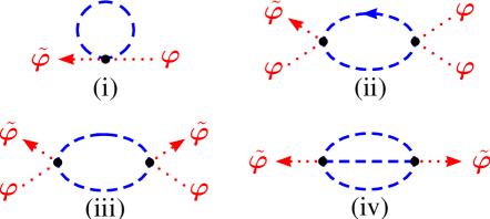
Figure 1: Graphs contributing to minus the effective action (56). Lines with and without an arrow represent the response and correlation propagators $R_{L}$ and $C_{L}$, respectively. Red dotted lines indicate $k=0$ components; blue broken lines $k\neq 0$ components (color online). For further explanations, see main text.

are the contributions implied by $\mathcal{J}_{\text{eff}}^{[1]}$ that involve two and four fields, respectively. Unlike graph (i), which is local in $\bm{y}$ and $t$, graphs (ii)–(iv) depend on the separations in $\bm{y}$ and $t$ between their two vertices (marked as black dots) and thus are nonlocal. Similar nonlocal contributions involving $6,8,\dotsc$ fields are contained in $\mathcal{J}_{\text{eff}}^{[1]}[\tilde{\bm{\varphi}},\bm{\varphi}]$. At one-loop order no modification of the Onsager coefficient $\mathring{\lambda}$ appears. However, the two-loop graph (iv) produces a nonlocal modification of it.

Let us use the notations

$$\gamma_{\tilde{\alpha}_{1},\dotsc,\alpha_{k}}^{(\tilde{k};k)}(\tilde{\bm{y}_{1}},\tilde{t}_{1};\dotsc;\bm{y}_{k},t_{k})$$ (61)

$$= \frac{\delta^{\tilde{k}+k}\mathcal{J}_{\text{eff}}}{\delta\tilde{\varphi}_{\tilde{\alpha}_{1}}(\bm{y}_{\tilde{\alpha}_{1}},\tilde{t}_{1})\dotsb\delta\varphi_{\alpha_{k}}(\bm{y}_{k},t_{k})}\Big{|}_{\tilde{\bm{\varphi}}=\bm{\varphi}=\bm{0}}$$

for the effective vertices of $\mathcal{J}_{\text{eff}}$, and write $\gamma^{(k)}_{\text{st}}(\bm{y}_{1},t_{1};\dotsc\bm{y}_{k},t_{k})$ for the analogously defined static effective $k$-point vertex functions (which were denoted by $\gamma^{(k)}$ in Ref. Grüneberg and Diehl, 2008) . By analogy with the bulk case, the vertex functions $\gamma^{(1;1)}(\dotsc;\omega)$ and $\gamma^{(1;3)}(\dotsc;\{\omega_{i}\})$ must satisfy the relations

$$\gamma^{(1;1)}(\dotsc;\omega=0)=\mathring{\lambda}\,\gamma^{(2)}_{\text{st}}(\dotsc)$$ (62)

and

$$\gamma^{(1;3)}(\dotsc;\{\omega_{i}=0\})=\mathring{\lambda}\,\gamma^{(4)}_{\text{st}}(\dotsc)\,,$$ (63)

where the ellipses stand for the positions $\bm{y}_{i}$ or momenta $\bm{p}_{i}$. The contribution of graph (i) to $\gamma^{(1;1)}(\dotso;\omega)/\mathring{\lambda}$ is independent of $\omega$ and hence agrees with that of its static analog to the static two-point vertex function $\gamma^{(2)}_{\text{st}}$. It gives an $L$-dependent shift of the temperature variable, changing it to

$$\mathring{\tau}^{(\wp)}_{L}(\mathring{\tau})=\mathring{\tau}+\frac{n+2}{6}\,\mathring{u}\,I_{1}^{(\wp)}(L;\mathring{\tau})\;,$$ (64)

where the integrals

$$I_{1}^{(\wp)}(L;\mathring{\tau})=\sum_{m\neq 0}\int_{\bm{p}}\int_{0}^{L}\frac{dz}{L}\,\frac{\lvert f_{m}^{(\wp)}(z)\rvert^{2}}{p^{2}+k_{m}^{2}+\mathring{\tau}}$$ (65)

for the two boundary conditions in question, $\wp=\text{per}$ and sp-sp, are given by

$$I^{(\mathrm{per})}_{1}(L;\mathring{\tau})=\frac{A_{d-1}}{L}\,\mathring{\tau}^{(d-3)/2}-A_{d}\,\mathring{\tau}^{(d-2)/2}+\frac{2\,Q_{d,2}(\mathring{\tau}L^{2})}{\mathring{\tau}L^{d}}$$ (66)

and

$$I^{\mathrm{(sp-sp)}}_{1}(L;\mathring{\tau})=I^{(\mathrm{per})}_{1}(2L;\mathring{\tau})\;,$$ (67)

respectively. Here we started to use the notational conventions summarized in Appendix A for momentum integrals such as $\int_{\bm{p}}$. Further,

$$A_{d}=\frac{2\,N_{d}}{4-d}=-(4\pi)^{-d/2}\,\Gamma(1-d/2)\;,$$ (68)

while $Q_{d,2}(r)$ is a special one of the functions defined byrem (d); Chamati et al. (1008)

$$Q_{d,\sigma}(r)\equiv\frac{r}{2}\left[\sum_{k\in 2\pi\mathbb{Z}}-\int_{-\infty}^{\infty}\frac{dk}{2\pi}\right]\int_{\bm{p}}\frac{(p^{2}+k^{2})^{\sigma/2-1}}{p^{2}+k^{2}+r}\;.$$ (69)

Using the definition (64), the result implied by Eqs. (3.20)–(3.24) of Ref. Grüneberg and Diehl, 2008 becomes

$$\gamma^{(1;1)}(\bm{p},\omega)/\mathring{\lambda}=p^{2}-i\omega/\mathring{\lambda}+\mathring{\tau}^{(\wp)}_{L}(\mathring{\tau})+\mathcal{O}(\mathring{u}^{2})\;.$$ (70)

For a discussion of the properties of the functions $Q_{d,\sigma}$ the reader is referred to Appendix D of Ref. Grüneberg and Diehl, 2008, where also plots of $Q_{4,2}(r)$ and $Q_{6,2}(r)$ are displayed (see Fig. 9 of this reference). It is known from previous worksKrech and Dietrich (1992); Grüneberg and Diehl (2008) that the above results yield the shifts (49) for $\mathring{\tau}=0$. This is easily verified utilizing the fact that

$$\lim_{r\to 0}Q_{d,2}(r)/r = \pi^{(d-5)/2}\,\Gamma[(3-d)/2]\,\zeta(3-d)/4$$ (71)

$$= \pi^{-d/2}\,\Gamma(d/2-1)\,\zeta(d-2)/4$$

(when $d\neq 1,3,5$) according to equation (B35) of Ref. Dantchev et al., 2006 and (C9) or (A15) of Ref. Grüneberg and Diehl, 2008.

It is equally easy to verify that the contribution of graph (ii) to $\gamma^{(1;3)}$ is in conformity with Eq. (63). Upon expressing $R_{L}(t)$ in terms of $\partial_{t}C_{L}$ via the fluctuation-dissipation relation (11), one arrives at the desired result $\int_{0}^{\infty}dt\,R_{L}(t)\,C_{L}(t)=(2\mathring{\lambda})^{-1}[C_{L}(t=0)]^{2}$.

Let us also note that the RG equations (29) for the functions $W^{(\tilde{N};N)}_{R}$ imply analogous ones for the renormalized vertex functions $\gamma^{(\tilde{k};k)}_{R}$. In the case of periodic boundary conditions, these vertex functions are evidently multiplicatively renormalizable. One has $\gamma^{(\tilde{k};k)}_{R}=Z_{\tilde{\phi}}^{\tilde{k}/2}Z_{\phi}^{k/2}\gamma^{(\tilde{k};k)}$, which leads to the RG equations

$$\bigg{[}\mathcal{D}_{\mu}-\tilde{k}\,\frac{\eta_{\tilde{\phi}}}{2}-k\,\frac{\eta_{\phi}}{2}\bigg{]}\gamma^{(\tilde{k};k)}_{R}=0\,.$$ (72)

For $\wp=\text{sp-sp}$ things are somewhat more subtle. It is known that $\Gamma^{(1,3)}$ has uv singularities corresponding to counterterms located on $\mathfrak{B}$ that are proportional to $\tilde{\bm{\phi}}\cdot\partial_{n}\bm{\phi}$ and $\bm{\phi}\cdot\partial_{n}\tilde{\bm{\phi}}$. Therefore, it is not multiplicatively renormalizable and does not satisfy a homogeneous RG equation.Diehl and Dietrich (1981); Symanzik (1981); Diehl and Dietrich (1983); Diehl (1986) However, when integrated with smooth background fields satisfying the boundary conditions (12) with $\mathring{c}_{1}=\mathring{c}_{2}=0$, the boundary singularities of the mentioned form give no contribution. The construction of $\mathcal{J}_{\text{eff}}[\tilde{\bm{\varphi}},\bm{\varphi}]$ involves integrations with such functions (namely, $\psi\psi$-propagators). Hence, the RG equations (72) carry over to the case of sp-sp boundary conditions.

They can be exploited in a standard fashion to obtain the scaling forms of the vertex functions $\gamma^{(\tilde{k},k)}(\{\bm{p}_{i},\omega_{i}\})$ for both types of boundary conditions $\wp=\text{per}$ and $\wp=\text{sp-sp}$. One obtains

$$\gamma_{R}^{(\tilde{k};k)}(\{\bm{p}_{i},\omega_{i}\};\tau,L)\approx\lambda\,\mu^{d_{\gamma}-2}$$ (73)

$$\times(\mu\xi_{\infty})^{-d_{\gamma}-\eta^{*}_{\gamma}}X^{(\wp)}_{\gamma}\big{(}\{\bm{p}_{i}\xi_{\infty};\omega_{i}/\Omega_{c}\};L/\xi_{\infty}\big{)}\phantom{(4.23)}$$

with

$$d_{\gamma} = 2-\tilde{k}+k-\frac{d-1}{2}(\tilde{k}+k-2)\;,$$

$$\eta_{\gamma}^{*} = (\tilde{k}+k)\eta/2+(\tilde{k}-1)(\mathfrak{z}-2)/2\,,$$ (74)

and the characteristic bulk frequency

$$\Omega_{c}=\lambda\,(\mu\xi_{\infty})^{-\mathfrak{z}}\,.$$ (75)

V Scaling functions of finite-size susceptibilities

We are now ready to turn to the computation of scaling functions by means of the small-$\epsilon$ expansion. We first consider the scaling function of the dynamical response function $\mathring{\lambda}\langle\bm{\varphi}\cdot\tilde{\bm{\varphi}}\rangle$ at the bulk critical point.

V.1 Dynamical finite-size response function

Noting that the $O(n)$ symmetry is unbroken when $T\geq T_{c,\infty}$, we set $\alpha=\beta=1$ in the response and vertex functions $W^{(1;1)}_{\alpha\beta}$ and $\gamma^{(1;1)}_{\alpha\beta}$ to obtain

$$\frac{\mathring{\lambda}}{n}\,\langle\bm{\varphi}\cdot\tilde{\bm{\varphi}}\rangle=\frac{1}{L}\int_{0}^{L}dz\int_{0}^{L}dz^{\prime}\,W^{(1;1)}_{11}\;.$$ (76)

The $\bm{p}\omega$-transform of this quantity gives us the finite-size susceptibility

$$\chi_{L}(p,\omega) = \int_{0}^{L}\frac{dz_{1}}{L}\int_{0}^{L}dz_{2}\int d^{d-1}y_{12}\int dt_{12}$$ (77)

$$\times\frac{\delta\langle\phi_{1}(\bm{x}_{1},t_{1})\rangle}{\delta h_{1}(\bm{x}_{2},t_{2})}\,e^{i(\omega t_{12}-\bm{p}\cdot\bm{y}_{12})}$$

The perturbation series of its inverse to order $o(\mathring{u}^{2})$ can be written as

$$[\chi^{(\wp)}_{L}(p,\omega)]^{-1} = \frac{-i\omega}{\mathring{\lambda}}+p^{2}+\mathring{\tau}^{(\wp)}_{L}+\frac{n+2}{6}\,\frac{\mathring{u}}{L}$$ (78)

$$\times G_{\infty}^{(d-1)}\big{(}\bm{0}|\mathring{\tau}_{L}^{(\wp)}\big{)}+o(\mathring{u}^{2})\;,\phantom{(5.3)}$$

where

$$G_{\infty}^{(d-1)}\big{(}\bm{0}|\mathring{\tau})=-A_{d-1}\,\mathring{\tau}^{(d-3)/2}$$ (79)

is the static bulk propagator in $d-1$ dimensions

$$G_{\infty}^{(d-1)}(\bm{y}|\mathring{\tau}) = \int_{\bm{p}}\,(p^{2}+\mathring{\tau})^{-1}\,e^{i\bm{p}\cdot\bm{y}}$$ (80)

$$= \frac{\left(\mathring{\tau}/y^{2}\right)^{(d-3)/4}}{(2\pi)^{(d-1)/2}}\,K_{(d-3)/2}\big{(}y\sqrt{\mathring{\tau}}\big{)}\,,\qquad$$

taken at zero separation $\bm{y}$.

From the RG equations (29) one concludes that the renormalized function $\chi_{L,R}^{(\wp)}$ has the asymptotic scaling form

$$\chi^{(\wp)}_{L,R}(p,\omega;\tau)\approx\mu^{-\eta}L^{2-\eta}\,\Xi^{(\wp)}(pL,\omega/\omega_{L},L/\xi_{\infty})\,,$$ (81)

where we have introduced the characteristic finite-size frequency

$$\omega_{L}=\lambda\,(\mu L)^{-\mathfrak{z}}\;.$$ (82)

Using the above result (78), one can verify that this scaling form complies with the small-$\epsilon$ expansion. At the order of our present calculation, the renormalization factors $Z_{\phi}$, $Z_{\lambda}$, and $Z_{u}$ can all be substituted by unity, but we needDiehl (1986)

$$Z_{\tau}=1+\frac{n+2}{3\epsilon}\,u+O(u^{2})$$ (83)

to first order in $u$. The pole term $\propto\mathring{\tau}u/\epsilon$ of $\mathring{\tau}_{L}$ gets cancelled when $\mathring{\tau}$ and $\mathring{u}$ are expressed in terms of renormalized quantities and the contribution from the counterterm $\propto Z_{\tau}Z_{\phi}-1$ is added. The associated renormalized shifts

$$\tau^{(\wp)}_{L}=\mu^{-2}Z_{\tau}^{-1}\mathring{\tau}^{(\wp)}_{L}$$ (84)

are uv finite; we obtain

$$\tau^{(\text{per})}_{L} = \tau^{(\text{sp-sp})}_{L/2}+O(u^{2})$$ (85)

$$= \tau+\tau\,\frac{n+2}{6}\,\frac{u}{\tau^{\epsilon/2}}\bigg{[}\frac{\tau^{\epsilon/2}-1}{\epsilon/2}+\frac{A_{d-1}}{\mu L\,\tau^{1/2}\,N_{d}}$$

$$+\frac{2\,Q_{d,2}(\mu^{2}\tau L^{2})}{(\mu^{2}L^{2}\,\tau)^{d/2}\,N_{d}}\bigg{]}+O(u^{2})\;.$$

Combining the above results then gives

$$[\chi_{L,R}^{(\wp)}(p,\omega)]^{-1}=\frac{-i\omega\mu^{2}}{\lambda}+p^{2}+r_{L}^{(\wp)}+O(u^{2})\;,$$ (86)

where

$$r^{(\wp)}_{L} = \mu^{2}\tau^{(\wp)}_{L}\Big{\{}1-\frac{n+2}{6}\,\frac{u\,A_{3-\epsilon}}{\mu LN_{4-\epsilon}}\,\big{[}\tau^{(\wp)}_{L}\big{]}^{-(1+\epsilon)/2}\Big{\}}$$ (87)

$$+O(u^{2})$$

are the inverse static finite-size susceptibilities.

Note that by keeping the $O(u)$ terms of $\tau^{(\wp)}_{L}$ in the contributions $\propto u\,[\tau^{(\wp)}_{L}]^{(1-\epsilon)/2}$, we have included contributions of order $u^{2}$ in these terms. While these results for $r^{(\wp)}_{L}$ differ from those of Ref. Grüneberg and Diehl, 2008 through precisely such terms, one easily checks that they reduce to Eqs. (4.31) and (4.32) of this reference when expanded to first order in $u$.

Our rationale for keeping the $O(u)$ contribution to the shift in the one-loop term associated with the zero mode should be clear. It prevents the propagator $G^{(d-1)}_{\infty}$ that it involves from becoming massless at bulk criticality when $L<\infty$. To compute the scaling functions $\Xi^{(\wp)}$, we must compute $\chi_{L}^{(\wp)}$ at the IR stable root $u^{*}=3\epsilon/(n+8)+O(\epsilon^{2})$ of the beta function $\beta_{u}$, where we can exploit the facts that both $\mathfrak{z}-2$ and $\eta$ are of order $\epsilon^{2}$. When $\tau>0$, the shifted temperature variable $\mathring{\tau}^{(\wp)}_{L}$ is of zeroth order in $u$. If we insert it into the contribution $\propto u[\tau^{(\wp)}_{L}]^{(\epsilon-1)/2}$, the $O(\epsilon)$ term of $\tau_{L}^{(\wp)}|_{u=u^{*}}$ will therefore produce an $O(\epsilon^{2})$ contribution. However, at criticality $\tau=0$, $\mathring{\tau}^{(\wp)}_{L}$ is linear in $u$ and hence of order $u^{*}=O(\epsilon)$ when evaluated at $u^{*}$. Accordingly, a contribution of order $\epsilon^{3/2}$ results from this source.

Proceeding as indicated above, one arrives at the results

$$[\Xi^{(\wp)}(\mathsf{p},w,\mathsf{L})]^{-1} = \mathsf{p}^{2}-iw+X^{(\wp)}_{\epsilon}(\mathsf{L})\Big{\{}1$$ (88)

$$-2\pi\,\epsilon\,\frac{n+2}{n+8}\,\big{[}X^{(\wp)}_{\epsilon}(\mathsf{L})\big{]}^{-1/2}\Big{\}}\qquad$$

with

$$X_{\epsilon}^{(\text{per})}(\mathsf{L}) = 4\,X_{\epsilon}^{(\text{sp-sp})}(\mathsf{L}/2)$$ (89)

$$= \mathsf{L}^{2}+\epsilon\,\frac{n+2}{n+8}\,\frac{16\pi^{2}\,Q_{4,2}(\mathsf{L}^{2})+2\pi\,\mathsf{L}^{3}}{\mathsf{L}^{2}}\,.\phantom{(5.14)}$$

The latter functions have the asymptotic behaviors

$$X_{\epsilon}^{(\wp)}(\mathsf{L})\underset{\mathsf{L}\to\infty}{\approx}\mathsf{L}^{2}\big{[}1+O(\mathsf{L}^{-1})\big{]}$$ (90)

and

$$X_{\epsilon}^{(\wp)}(\mathsf{L})\underset{\mathsf{L}\to 0}{\approx}\frac{2\pi^{2}}{3a^{2}_{\wp}}\,\frac{n+2}{n+8}\,\epsilon\;,$$ (91)

where $a_{\wp}$ is given by

$$a_{\wp}=\begin{cases}1&\text{for }\wp=\text{per}\,,\\ 2&\text{for }\wp=\text{sp-sp}\,.\end{cases}$$ (92)

Setting $\mathsf{p}=w=0$ in Eq. (88) gives us the scaling functions of the static finite-size susceptibilities. One easily verifies that our results for $\mathsf{L}^{2}/\Xi^{(\wp)}(0,0,\mathsf{L})$ are in conformity with the $O(\epsilon)$ expressions (4.46) and (4.47) of Ref. Grüneberg and Diehl, 2008.

The limiting behavior (91) implies that the scaling functions (88) become

$$[\Xi^{(\wp)}(\mathsf{p},w,0)]^{-1} = \mathsf{p}^{2}-iw+\frac{2\pi^{2}}{3\,a_{\wp}^{2}}\,\frac{n+2}{n+8}\bigg{[}\epsilon$$ (93)

$$-\sqrt{6}\,a_{\wp}\,\Big{(}\frac{n+2}{n+8}\Big{)}^{1/2}\,\epsilon^{3/2}\bigg{]}$$

$$+o(\epsilon^{3/2})$$

at $\mathsf{L}=0$, which explicitly shows the announced $O(\epsilon^{3/2})$ contributions. Before we embark on a discussion of this result, let us note that the scaling functions of the correlation function

$$C^{(\wp)}_{L}(p,\omega) = \int_{0}^{L}\frac{dz_{1}}{nL}\int_{0}^{L}dz_{2}\int d^{d-1}y_{12}\int dt_{12}$$

$$\times\langle\bm{\phi}(\bm{x}_{1},t_{1})\cdot\bm{\phi}(\bm{x}_{2},t_{2})\rangle^{\text{cum}}\,e^{i(\omega t_{12}-\bm{p}\cdot\bm{y}_{12})}$$

need no separate calculations since the fluctuation-dissipation relation (11) in conjunction with Eq. (81) yields

$$C^{(\wp)}_{L}(p,\omega)\approx\mu^{-\eta}L^{2-\eta}\,\frac{2}{w}\,\text{Im}\,\Xi^{(wp)}(\mathsf{p},w)\;.$$ (95)

Had we computed the expansions (93) merely to linear order in $\epsilon$, one might be tempted to think that even the direct evaluation of these truncated series at $d=3$ would give acceptable estimates. The $O(\epsilon^{3/2})$ terms reveal that there is no reason for such optimism: their signs differ from those of the contributions linear in $\epsilon$. Furthermore, their coefficients are quite large. Thus, evaluating the series expansion (93) to order $\epsilon^{3/2}$ at $\epsilon=1$ yields (unphysical) negative values even for $n=1$, albeit the results remain positive when $\epsilon$ is sufficiently small. This shows that more sophisticated extrapolation techniques are needed to obtain reliable estimates for these quantities at $d=3$.

An important check of the results for periodic boundary conditions can be made by comparing them with the exact large-$n$ results obtained from the solution of the mean spherical model with short range interactions.Brankov et al. (2000); Dantchev et al. (2006); Chamati et al. (1008) As we will show now, the large-$n$ limit of the small-$\epsilon$ expansion (93) for $\wp=\text{per}$ can be recovered by solving the self-consistent equation that the finite-size susceptibility obeys in the limit $n\to\infty$ for $d=4-\epsilon$ in an iterative fashion.

There are two reasons why a similar comparison with large-$n$ results cannot be made here in the case of sp-sp boundary conditions. First, translation invariance perpendicular to the boundary planes is broken for these boundary conditions, just as it generally is for free boundary conditions. The large-$n$ limit therefore corresponds to a modified spherical lattice model involving separate constraintsKnops (1973); rem (d) for the averages of $\sum_{i\in\text{layer }z}S_{i}^{2}$ in each layer $z$, where $S_{i}$ is a spin variable on site $i$. Second, when $d=3$, the thermal fluctuations should prevent the occurrence of film and surface phases with long-range order at temperatures $T>0$ in the continuous symmetry case $n>1$ and hence for $n\to\infty$. Hence sp-sp boundary conditions cannot be realized when $d=3$ and $n=\infty$.

V.2 Comparison with exact spherical-model results for periodic boundary conditions

An important check of our results for periodic boundary conditions is their comparison with exact spherical-model results. The static finite-size susceptibility of the spherical model on a $d$-dimensional slab with periodic boundary conditions can be written as

$$\chi_{L}^{(\text{SM})}=L^{2}/X^{\text{SM}}_{d}(L/\xi_{\infty})\;,$$ (96)

where the scaling function $X^{\text{SM}}_{d}(\mathsf{L})$ is a solution [see, eg., equations (5.2) and (4.66) of Refs. Grüneberg and Diehl, 2008 and Dantchev et al., 2006, respectively]

$$2\,Q_{d,2}(X^{\text{SM}}_{d})/X^{\text{SM}}_{d}=A_{d}\,\big{[}\big{(}X^{\text{SM}}_{d}\big{)}^{(d-2)/2}-\mathsf{L}^{d-2}\big{]}\;.$$ (97)

For $d=3$, the solution can be obtained in closed form;Dantchev et al. (2006); rem (d) it reads

$$X^{\text{SM}}_{3}(\mathsf{L}) = 4\,\mathrm{arccsch}^{2}\big{(}2\,e^{-\mathsf{L}/2}\big{)}$$ (98)

$$= 4\ln^{2}\Big{[}\frac{1}{2}\Big{(}e^{\mathsf{L}/2}+\sqrt{4+e^{\mathsf{L}}}\Big{)}\Big{]}\,.$$

Its critical value, which corresponds to the amplitude $1/\Xi^{\text{(per)}}(0,0,0)$, isChamati et al. (1008)

$$X^{\text{SM}}_{3}(0)=4\ln^{2}g\simeq 0.926259\;,\quad g=\big{(}1+\sqrt{5}\,\big{)}/2\;,$$ (99)

where $g$ is the golden mean.

To determine the amplitude $X^{\text{SM}}_{d}(0)$ in $d=4-\epsilon$ dimensions, we substitute the series expansion of the function $Q_{d,2}(r)$ given in equation (C.9) of Ref. Grüneberg and Diehl, 2008 to obtain the representation

$$\frac{2\,Q_{4-\epsilon,2}(r)}{r}=A_{4-\epsilon}\,r^{1-\epsilon/2}-A_{3-\epsilon}\,r^{(1-\epsilon)/2}+f_{\epsilon}(r)$$ (100)

with

$$f_{\epsilon}(r)=\sum_{j=0}^{\infty}b^{(j)}_{\epsilon}\,r^{j}\;,$$ (101)

where

$$b^{(j)}_{\epsilon}=\frac{(-1)^{j}\,\Gamma[j+(\epsilon-1)/2]}{j!\,2^{2j+1}\,\pi^{2j+(\epsilon+1)/2}}\,\zeta(2j+\epsilon-1)\;.$$ (102)

The coefficients $A_{4-\epsilon}$ and $b_{\epsilon}^{(1)}$ have simple poles at $\epsilon=0$ whose residues differ by the factor $(-2)$, so that the pole term of $A_{4-\epsilon}\,r^{1-\epsilon/2}$ cancels that of $b^{(1)}_{\epsilon}r$. The remaining coefficients, $A_{3-\epsilon}$ and $b_{\epsilon}^{(j)}$ with $j\neq 1$, are regular at $\epsilon=0$. On the other hand, $A_{3-\epsilon}$ and $b^{(0)}_{\epsilon}$ have simple poles at $\epsilon=1$ whose residues are equal.

These results imply that $X_{4-\epsilon}(\mathsf{L})-\mathsf{L}^{2}$ must vanish linearly as $\epsilon\to 0$, so that the right-hand side of Eq. (97) approaches a nonzero limit. The $O(\epsilon)$ term of $X_{4-\epsilon}(\mathsf{L})-\mathsf{L}^{2}$ was computed in Ref. Grüneberg and Diehl, 2008 [see its Eq. (5.3)]. To determine the $O(\epsilon^{3/2})$ contribution to $X_{4-\epsilon}(0)$, we set $\mathsf{L}=0$ and solve Eq. (97) with the ansatz $X_{4-\epsilon}(0)=C_{1}\epsilon+C_{3/2}\epsilon^{3/2}+o(\epsilon^{3/2})$. This gives

$$X^{\text{SM}}_{4-\epsilon}(0)=\frac{2\pi^{2}}{3}\big{(}\epsilon-\sqrt{6}\,\epsilon^{3/2}\big{)}+o(\epsilon^{3/2})\;.$$ (103)

Obviously, the result agrees with the expansion (93) of $[\Xi^{(\text{per})}(\mathsf{p},w,0)]^{-1}$ for $n=\infty$.

V.3 Dynamical finite-size surface response function

In Sec. V B we were concerned with the dynamic finite-size susceptibilities (77). These are integral quantities. As an alternative, we here wish to consider the local susceptibilities $\chi^{(\text{sp-sp})}_{11}=\mathring{\lambda}\,\langle\bm{\phi}^{\mathfrak{B}_{1}}(\bm{y},t)\cdot\tilde{\bm{\phi}}^{\mathfrak{B}_{1}}(\tilde{\bm{y}},\tilde{t\,})\rangle/n$ and $\chi^{(\text{sp-sp})}_{1L}=\mathring{\lambda}\,\langle\bm{\phi}^{\mathfrak{B}_{1}}(\bm{y},t)\cdot\tilde{\bm{\phi}}^{\mathfrak{B}_{2}}(\tilde{\bm{y}},\tilde{t\,})\rangle/n$ describing the linear responses of the order-parameter density at one boundary plane to a magnetic field acting on the order-parameter density in the same and the complementary boundary planes, respectively. In the case of periodic boundary conditions, both quantities are the same — and by translational invariance along the $z$-direction — identical with the layer susceptibility $\chi_{zz}=\mathring{\lambda}\,\langle\bm{\phi}(\bm{y},z,t)\cdot\tilde{\bm{\phi}}(\tilde{\bm{y}},z,\tilde{t\,})\rangle/n$ for any layer $z$. We start with an investigation of the latter. For the sake of simplicity, we do not consider deviations from the bulk critical temperature here, setting $\tau=0$.

V.3.1 Layer susceptibility for periodic boundary conditions

Our analysis of the finite-size susceptibility $\chi_{L}$ suggests that we should work with a dressed $\varphi\varphi$-propagator that accounts for the $O(\mathring{u})$ shift $\mathring{\tau}^{(\text{per})}_{L}$ given in Eq. (49). Noting that the $k_{0}=0$-mode contribution to $C_{L}(\bm{p}=\bm{0};z=0;t=0)$ vanishes when $\mathring{\tau}=0$, one sees that a single two-loop graph suffices to capture all contributions to order $\epsilon^{3/2}$ in the renormalized quantity $\chi_{zz,R}$. One obtains

$$\chi_{zz}(p,\omega;L)/\mathring{\lambda} = \frac{\coth(\mathring{\kappa}_{\omega}L/2)}{2\mathring{\lambda}\mathring{\kappa}_{\omega}}+\raisebox{-8.53581pt}{\includegraphics[scale={0.8}]{oneloopchizzpsi.eps}}$$ (104)

$$+\raisebox{-8.53581pt}{\includegraphics[scale={0.8}]{oneloopchizzvarphi.eps}}+O(\mathring{u}^{2})\;,$$

where $\mathring{\kappa}_{\omega}$ now denotes the quantity (24) with $\mathring{\tau}$ set to zero. Here full black lines with and without arrows represent the free response and correlation propagators $R_{L}$ and $C_{L}$ with $\mathring{\tau}=0$, respectively. The dashed blue line indicates $C^{(\text{per})}_{L,\psi}$ with $\mathring{\tau}=0$. The dotted red line is the $k=0$ part of $C^{(\text{per})}_{L}$ with $\mathring{\tau}=\delta\mathring{\tau}^{(\text{per})}_{L}$. Note that we do not include the shift $\delta\tau^{(\text{per})}_{L}$ in the $k=0$ contributions to the external legs of the two graphs. Their inclusion would produce terms of order $\mathring{u}^{2}$ and hence lead to corrections of order $\epsilon^{2}$.

In Appendix C the graphs in Eq. (104) are computed. From the results given in Eqs. (137) and (138), the RG-improved perturbation expansion of the renormalized dynamic layer susceptibility $\chi_{zz,R}=\chi_{zz}/Z_{\phi}$ follows in a straightforward fashion. Evaluating it at the fixed-point value, one sees that it is in conformity with the scaling form predicted by the RG equations (29), namely

$$\chi^{(\text{per})}_{zz,R}(p,\omega;L,\tau=0)\approx\mu^{\eta}L^{1-\eta}\,\Xi_{zz}^{(\text{per})}(pL,\omega/\omega_{L})\;.$$ (105)

where the scaling function has the small-$\epsilon$ expansion

$$\Xi_{zz}^{(\text{per})}(\mathsf{p},w) = \frac{\coth(\varkappa/2)}{2\varkappa}-\frac{\pi^{2}}{12}\,\frac{n+2}{n+8}\,\frac{\varkappa+\sinh\varkappa}{\varkappa^{3}\sinh^{2}(\varkappa/2)}$$ (106)

$$\times\left[\epsilon-\sqrt{6\,\frac{n+2}{n+8}}\,\epsilon^{3/2}\right]+o(\epsilon^{3/2})\phantom{(5.23)}$$

with

$$\varkappa=\sqrt{\mathsf{p}^{2}-iw}\;.$$ (107)

The susceptibility $\chi_{zz,R}$ must reduce to an $L$-independent bulk quantity as $L\to\infty$. Therefore, the scaling function should have the limiting behavior

$$\Xi_{zz}^{(\text{per})}(\mathsf{p},w)\underset{\mathsf{p}\to\infty}{\approx}\mathsf{p}^{\eta-1}\,\Psi(w\mathsf{p}^{-\mathfrak{z}})\;.$$ (108)

Equation (108) shows that this is indeed the case, giving

$$\Psi(w\mathsf{p}^{-\mathfrak{z}})=\frac{1}{2\sqrt{1-iw\mathsf{p}^{-\mathfrak{z}}}}+O(\epsilon^{2})\;,$$ (109)

which is the correct bulk result.

As long as $L$ is finite, there is no reason for $\chi_{zz,R}$ to diverge at the bulk critical temperature. Hence, we expect its inverse $1/\chi_{zz,R}(p,0;L,0)$ to approach a nonzero limit. From Eq. (106) we can read off the small-$\epsilon$ expansion of $1/\Xi_{zz}^{(\text{per})}(\mathsf{p},w)$ and compute its limit

$$\lim_{\mathsf{p}\to 0}\frac{1}{\Xi_{zz}^{(\text{per})}(\mathsf{p},0)} = \frac{2\pi^{2}}{3}\,\frac{n+2}{n+8}\left[\epsilon-\sqrt{6\,\frac{n+2}{n+8}}\,\epsilon^{3/2}\right]$$ (110)

$$+o(\epsilon^{3/2})\,.$$

The result agrees at this order with the expansion (93) of the inverse static susceptibility $[\Xi^{(\text{per})}(0,0,0)]^{-1}$. Thus the inverse static zero-momentum layer susceptibility $1/\chi_{zz,R}(0,0;L,0)$ is indeed nonzero. Of course, the previously discussed difficulties to obtain reliable $d=3$ estimates from this expansion to the order $\epsilon^{3/2}$ apply here as well.

V.3.2 Surface susceptibilities for sp-sp boundary conditions

The graphs of the surface susceptibilities $\chi^{(\text{sp-sp})}_{11}$ and $\chi^{(\text{sp-sp})}_{1L}$ corresponding to the ones displayed in Eq. (104) are computed in Appendix C.2. The results are gathered in Eqs. (160)–(162). Using them one can verify in a straightforward manner that the renormalized susceptibilities $\chi^{(\text{sp-sp})}_{11,R}=\chi^{(\text{sp-sp})}_{11}/Z_{\phi}Z_{1}$ and $\chi^{(\text{sp-sp})}_{1L,R}=\chi^{(\text{sp-sp})}_{1L}/Z_{\phi}Z_{1}$ are uv finite to the appropriate order in $u$. One obtains

$$\chi^{(\text{sp-sp})}_{11,R} = \frac{\coth(\kappa_{\omega}L)}{\kappa_{\omega}}-\frac{n+2}{6}\,u\bigg{\{}\frac{\coth(\kappa_{\omega}L)}{\kappa_{\omega}}\,\Big{[}1-2\gamma_{E}$$ (111)

$$-2\ln(\mu L)]+S(\kappa_{\omega}L)+R(\kappa_{\omega}L)$$

$$+\frac{\pi^{2}}{3}\bigg{[}1-\frac{4}{L}\,\bigg{(}\frac{n+2}{2\mu^{2}L^{2}}\,u\bigg{)}^{1/2}\bigg{]}I_{1,1}(\kappa_{\omega}L)$$

$$+O(\epsilon)\bigg{\}}$$

and

$$\chi^{(\text{sp-sp})}_{1L,R} = \frac{\text{csch}(\kappa_{\omega}L)}{\kappa_{\omega}}-\frac{n+2}{6}\,u\bigg{\{}\frac{\text{csch}(\kappa_{\omega}L)}{\kappa_{\omega}}\,[1-2\gamma_{E}$$ (112)

$$-2\ln(\mu L)]+2S_{1,2}^{(0)}(\kappa_{\omega}L)+R_{2}(\kappa_{\omega}L)$$

$$+\frac{\pi^{2}}{3}\bigg{[}1-\frac{4}{L}\,\bigg{(}\frac{n+2}{2\mu^{2}L^{2}}\,u\bigg{)}^{1/2}\bigg{]}I_{1,2}(\kappa_{\omega}L)$$

$$+O(\epsilon)\bigg{\}}\,,$$

where $\kappa_{\omega}=\sqrt{p^{2}-i\omega\mu^{2}/\lambda}$, while $S(\varkappa)$, $R(\varkappa)$, $I_{1,1}(\varkappa)$, $S_{1,2}^{(0)}(\varkappa)$, $R_{2}(\varkappa)$, and $I_{1,2}(\varkappa)$ denote the functions specified by Eqs. (157), (158), (143), (155), (159), and (144), respectively. The functions $R(\varkappa)$ and $R_{2}(\varkappa)$ are single integrals, which can be computed by numerical integration.

According to the RG equations (29) these susceptibilities should have the asymptotic scaling behavior

$$\chi^{(\text{sp-sp})}_{\begin{subarray}{c}11,R\\ 1L,R\end{subarray}}(p,\omega;L,\tau=0)\approx\mu^{-\eta_{\|}^{\text{sp}}}L^{1-\eta_{\|}^{\text{sp}}}\,X_{\begin{subarray}{c}11\\ 1L\end{subarray}}(pL,\omega/\omega_{L})\;,$$ (113)

where $\eta_{\|}^{\text{sp}}$ is a standard surface correlation exponent associated with the special transition whose $\epsilon$ expansion $\eta_{\|}^{\text{sp}}=-\epsilon\,(n+2)/(n+8)+O(\epsilon^{2})$ is knownDiehl and Dietrich (1981, 1983); Diehl (1986) to order $\epsilon^{2}$. Evaluating the above results (111) and (112) at $u^{*}$ shows their consistency with these scaling forms and yields the small-$\epsilon$ expansions

$$X_{11}(\mathsf{p},w) = \frac{\coth\varkappa}{\varkappa}-\frac{n+2}{n+8}\,\frac{\epsilon}{2}\,\bigg{\{}(1-2\gamma_{E})\,\frac{\coth\varkappa}{\varkappa}$$ (114)

$$+S(\varkappa)+R(\varkappa)$$

$$+\frac{\pi^{2}}{3}\,\bigg{[}1-2\Big{(}6\epsilon\,\frac{n+2}{n+8}\Big{)}^{1/2}\bigg{]}I_{1,1}(\varkappa)$$

$$+o(\epsilon^{3/2})\bigg{\}}\phantom{(5.31)}$$

and

$$X_{1L}(\mathsf{p},w) = \frac{\text{csch}\varkappa}{\varkappa}-\frac{n+2}{n+8}\,\frac{\epsilon}{2}\,\bigg{\{}(1-2\gamma_{E})\,\frac{\text{csch}\varkappa}{\varkappa}$$ (115)

$$+2S^{(0)}_{1,2}(\varkappa)+R_{2}(\varkappa)$$

$$+\frac{\pi^{2}}{3}\,\bigg{[}1-2\Big{(}6\epsilon\,\frac{n+2}{n+8}\Big{)}^{1/2}\bigg{]}I_{1,2}(\varkappa)$$

$$+o(\epsilon^{3/2})\bigg{\}}$$

where $\varkappa$ is again given by Eq. (107).

In the limit $\mathsf{p}\to\infty$, the function $X_{11}$ must behave as

$$X_{11}(\mathsf{p},w)\underset{\mathsf{p}\to\infty}{\approx}\mathsf{p}^{\eta_{\|}^{\text{sp}}-1}\,\Psi_{11}(w\mathsf{p}^{-\mathfrak{z}})\,,$$ (116)

where $\Psi_{11}$ must agree with the scaling function of $\chi^{(\text{sp-sp})}_{11,R}$ of the semi-infinite ($L=\infty$) theory. This is indeed the case. The limit $\lim_{\mathsf{p}\to\infty}\mathsf{p}^{1-\eta_{\|}^{\text{sp}}}\Psi_{11}(\mathsf{p},w)$ can be computed in a straightforward fashion, giving

$$\Psi_{11}(v)=\frac{1}{\sqrt{1-iv}}\Big{\{}1+\frac{\epsilon}{2}\,\frac{n+2}{n+8}\,[1-\ln(4-4iv)]\Big{\}}+O(\epsilon^{2})\;.$$ (117)

An independent calculation for the semi-infinite theory yields precisely the same result.

Since $\chi^{(\text{sp-sp})}_{1L,R}$ vanishes as $L\to\infty$, the analog of the scaling function $\psi_{11}$ for $\chi^{(\text{sp-sp})}_{1L,R}$ must vanish. Checking the limit $\lim_{\mathsf{p}\to\infty}\mathsf{p}^{1-\eta_{\|}^{\text{sp}}}\Psi_{1L}(\mathsf{p},w)$ explicitly, we do in fact find that it is zero.

Just as the layer susceptibility $\chi_{zz,R}$, the surface susceptibilities $\chi^{(\text{sp-sp})}_{11,R}$ and $\chi^{(\text{sp-sp})}_{1L,R}$ should not become critical at the bulk critical point and hence have finite $p\to 0$ limits at $\tau=\omega$. To check this, we set $\omega=0$ in Eqs. (114) and (115), determine the series expansions of $[X_{11}(\mathsf{p},0)]^{-1}$ and $[X_{1L}(\mathsf{p},0)]^{-1}$ to $O(\epsilon^{3/2})$, and then take the limits $\mathsf{p}\to 0$. The results are

$$[X_{11,R}(0,0)]^{-1}=[X_{1L,R}(0,0)]^{-1}+o(\epsilon^{3/2})$$ (118)

$$= \epsilon\,\frac{\pi^{2}}{6}\,\frac{n+2}{n+8}\left[1-2\Big{(}6\epsilon\,\frac{n+2}{n+8}\Big{)}^{1/2}\right]+o(\epsilon^{3/2})\,.\phantom{(5.33)}$$

They indicate that an $L$-dependent shift of the multicritical special point occurs also along the $c$-direction, not only along the temperature direction. Note, however, that a special point at which a bulk disordered phase with long-range surface order meets with a bulk-disordered, surface-ordered phase and a bulk-ordered, surface-ordered phase exists for $d=3$ dimensional, semi-infinite spin systems only when $n=1$. The analog of this multicritical point for finite $L$ is the one where the transition temperature of the surface transition coincides with the transition temperature $T_{c,L}$ of the film.

VI Conclusions

In this article, we have studied model $A$ in film geometry. We focused on the cases of boundary conditions for which the classical (Landau-van Hove) theory involves zero modes: periodic boundary conditions and free boundary conditions with critically enhanced surface interactions.

Major motivations were to determine the consequences of the zero mode and to reformulate RG-improved perturbation theory such that a well-defined small-$\epsilon$ expansion results at the bulk critical temperature. Our reformulation of RG-improved perturbation theory builds on the strategy pursued in Refs. Diehl et al., 2006 and Ref. Grüneberg and Diehl, 2008 to investigate static properties such as the finite-size free energy and the Casimir force. In these papers it was shown that the conventional $\epsilon$-expansion breaks down and contributions involving half-integer powers $\epsilon^{k/2}$ with $k\geq 3$ modulo powers of $\ln\epsilon$ appear in the expansion of the critical Casimir amplitudes and other quantities. Here, we confirmed this breakdown and explicitly determined the small-$\epsilon$ expansions of various dynamic finite-size, layer, and surface susceptibilities at $T_{c,\infty}$ to order $\epsilon^{3/2}$. We were also able to cast the $\epsilon$-expansion of the temperature-dependent scaling functions of the finite-size susceptibilities $\chi^{(\wp)}_{L,R}$ for both boundary conditions $\wp=\text{per}$ and $\wp=\text{sp-sp}$ in a form that reproduce their expansions to order $\epsilon^{3/2}$ as $T\to T_{c,\infty}$.

Despite these successes, the theory suffers from severe limitations and is still in an unsatisfactory state. First of all, our results (110) and (118) for the inverse layer and surface susceptibilities at $T_{c,\infty}$ suggest that reliable estimates for $d=3$ can hardly been obtained on the basis of such small-$\epsilon$ expansion to order $\epsilon^{3/2}$ alone. Just as in the case of the Casimir amplitudes and the scaling function of the residual free energy at small values of $L/\xi_{\infty}$,Grüneberg and Diehl (2008) the deviations of the simplest extrapolations obtained by setting $\epsilon=1$ in the series truncated at the respective orders $\epsilon$ and $\epsilon^{3/2}$ appear to oscillate in sign. It is conceivable that the situation is particularly bad in those cases where the classical theory involves zero modes. These zero modes provide a separate source of IR singularities, a problem one also encounters in thermal field theory.Le Bellac (2004) It has been suggested to handle IR problems of this kind by a resummation of “foam” diagrams. In the case of the $n$-component bulk $\phi^{4}$ theory at finite temperature, Drummond et al. (1998) this procedure yields results for the pressure in conformity with the exact large-$n$ result. Whether and to what extent RG-improved perturbation theory might be improved by combining it with resummations of this kind remains to be seen.

Finally, let us emphasize that there is little reason to believe that the theory is in a much better state in those cases where the classical theory does not involve zero modes, notwithstanding the additional difficulties such modes cause. For free boundary conditions, one will generically encounter a zero mode in the classical theory at an $L$-dependent temperature $T^{(0)}_{c,L}\neq T_{c,\infty}$. This indicates that in Landau theory the film becomes critical at this temperature and undergoes a transition to an ordered low-temperature phase. The ordered phase and hence the transition to it may not survive the inclusion of thermal fluctuations when $L<\infty$. This happens in the continuous symmetry case $n>1$ when $d\leq 3$, where it should be recalled that the $d=3$ case with $n=2$ is special in that the film has a low-temperature phase with quasi-long-range order. However, even in those cases where the film does have a transition to an ordered low-temperature phase for finite $L$ (as it does when $d=3$ and $n=1$), one encounters two important challenges that are beyond the scope of the presently available analytical RG approaches but any satisfactory full theory of dimensional crossover must be able to cope with: (i) to determine the location of the singularity of the residual free energy’s scaling function corresponding to the transition temperature $T_{c,L}$ with acceptable accuracy, and (ii) to yield the correct IR singularities at this transition in conformity with the expected $(d-1)$-dimensional critical behavior of the film. The difficulty is that even the shift cannot normally be computed by perturbation theory but requires RG techniques to deal with the IR singularities.rem (e) The RG scheme employed here and in the work of Krech and DietrichKrech and Dietrich (1992) may be appropriate to go on scales of the order of $\xi_{\infty}$ as long as $\xi_{\infty}\lesssim L$. However, it is insufficient to integrate out degrees of freedom between $L$ and the film’s correlation length $\xi_{L}$ in an adequate fashion when $\xi_{L}>L$, and to correctly yield the IR singularities at the critical temperature $T_{c,L}$ even when the boundary conditions do not involve zero modes at $T_{c,\infty}$.

We close with some comments on the universality of our results and finite-size scaling results in general. Chen and DohmChen and Dohm (2002); Dohm (2008) recently launched a discussion of the universality of finite-size scaling results and the validity of two-scale (and multiscale) factor universality. Let us consider their concerns in some detail. A first issue raised in Ref. Chen and Dohm, 2002 is that the use of a sharp large-momentum cutoff modifies the $L$ dependence of the singular part of the finite-size free energy density of systems of linear size $L$ in a qualitative manner. This effect is unphysical and entirely due to the use of a sharp cutoff; that a sharp cutoff can produce unphysical effects has been known since the early days of Wilson’s RG.Wilson and Kogut (1974) For systems of the kind considered by them — systems that are finite in all directions — the issue was discussed and clarified in Refs. Dantchev and Rudnick, 2001 and Dantchev et al., 2003. It needs no further discussion.

A second point made in Refs. Chen and Dohm, 2002 is that long-range interactions which are irrelevant in the RG sense produce algebraically decaying contributions to the singular part of the finite-size free energy density. Such interactions were previously considered by Dantchev and co-workers,Dantchev and Rudnick (2001); Chamati and Dantchev (2002) who introduced the term “subleading long-range interaction” for them. Away from criticality, these contributions compete with the exponentially decaying ones one has for systems with purely short-range interactions and become dominant in the appropriate region of temperature and large $L$. While such contributions (which are expected to be small on an absolute scale) still have to be clearly verified by experiments, they certainly are real.

Chen and DohmChen and Dohm (2002) interpreted their presence as signaling the breakdown of finite-size scaling. However, what is broken is just the simple version of finite-size scaling that involves a single length besides $L$, namely, the correlation length. Subleading long-range interactions give rise to at least one further length — the one associated with the corresponding irrelevant scaling field.rem (d) This must not be set to zero in order to retain the long-range tail in the regime where it dominates the exponentially decaying short-range contribution to the finite-size free-energy density. It may well be set to zero in the critical regime $L/\xi_{\infty}\ll 1$ because the subleading long-range interaction contributes there only a correction to the leading $L$ dependence. Thus, subleading long-range interactions are intermediate between dangerous irrelevant and conventional irrelevant perturbations: they share with the former the property that they must not generally be set to zero. Unlike those (which would affect the leading critical behavior of some quantities), but similar to the latter, they give only corrections to the leading critical behavior.

Note that the mechanism just described for subleading long-range interactions is neither specific to finite-size critical behavior nor new. A familiar analog known from the study of critical adsorption of fluids was discussed more than 25 years ago by de Gennes.de Gennes (1981) Substrates (“walls”) typically exert one-body forces on the fluid that have besides short-range components algebraically decaying van-der-Waals tails. In a semi-infinite geometry bounded by a wall at $z=0$ and restricted to $z\geq 0$, the latter contribute effective wall-fluid interactions of the form $\int d^{d-1}y\int_{0}^{\infty}dz\,h_{\text{wf}}(z)\,\phi(\bm{y},z)$ to the Hamiltonian, where $h_{\text{wf}}(z)$ behaves as $A_{\text{wf}}\,z^{-\upsilon}$ as $z\to\infty$ (cf. Ref. Peliti and Leibler, 1983 and Sec. 3.11 of Ref. Diehl, 1986). The long-range part is irrelevant in the RG sense provided the exponent $\upsilon$ is larger than the magnetic RG eigenexponent $y_{h}=(d+2-\eta)/\nu$, which is the case for nonretarded and retarded van-der-Waals interactions in $d=3$ dimensions (for which $\upsilon=3$ and $\upsilon=4$, respectively). It produces a long-range tail $\sim z^{-\upsilon}$ to the deviation $\delta m(z)=m(z)-m(\infty)$ of the order-parameter density $m(z)=\langle\phi(\bm{y},z)\rangle$ from its bulk value $m(\infty)$. By setting the length $\sim g_{\text{wf}}^{\upsilon-y_{h}}$ associated with the irrelevant scaling field $g_{\text{wf}}\sim A_{\text{wf}}$ to zero, one would loose this algebraically decaying contribution. On the other hand, the leading temperature singularity $\sim|\tau|^{-(\nu-\beta)}$ of the excess order parameter $\int_{0}^{\infty}dz\,\delta m(z)$ would remain the same since $g_{\text{wf}}$ yields merely corrections to scaling for this quantity. The analogy with how subleading long-range interactions affect finite-size properties is obvious. Of course, the amplitude of the irrelevant scaling field $g_{\text{wf}}$ is nonuniversal. Following the logic of Refs. Chen and Dohm, 2002 and Dohm, 2008, one would have to call this a violation of scaling in semi-infinite systems, though it again just means that single-length scaling reaches its limits, failing to capture the asymptotic behavior of certain quantities.

To what extent would the inclusion of subleading long-range interactions alter the results of our analysis of dynamic finite-size critical behavior given above? While a detailed, quantitative analysis of their effects is beyond the scope of this paper, clear predictions can be made on general grounds and the basis of what is known from statics. Power laws describing asymptotic dependences in $L$ or $\tau$ at $T=T_{c,\infty}$ will be modified by corrections to scaling involving the associated irrelevant scaling field.rem (d) For a subleading long-range pair interaction decaying $\sim x^{-(d+\sigma)}$ (with $\sigma>2-\eta$), the associated correction-to-scaling exponent is $\omega_{\sigma}=\sigma-2+\eta$ (see, e.g., Ref. Dantchev et al., 2006 and its references). Thus these corrections should be down by factors $L^{-\omega_{\sigma}}$ (or $\xi_{\infty}^{-\omega_{\sigma}}$) in comparison to the respective leading power laws. Correspondingly, scaling forms such as the one for the finite-size susceptibility $\chi^{(\wp)}_{L,R}(p,\omega;\tau)$ given in Eq. (81) should obtain a correction $\propto L^{2-\eta-\omega_{\sigma}}\,\Xi_{\sigma}^{(\wp)}(pL,\omega/\omega_{L},L/\xi_{\infty})$ at linear order in the irrelevant long-range scaling field.rem (d) Furthermore, there exist quantities whose behaviors get qualitatively modified by subleading long-range interactions. This is typically the case (in certain regimes of $L$ and $\tau$) for quantities that decay exponentially in the absence of long-range interactions. Obvious examples are zero-frequency response functions in position space at temperatures $\tau>0$; these decay algebraically in the limit of large distances $x_{ij}=|\bm{x}_{i}-\bm{x}_{j}|\to\infty$ between two points when the pair interactions have a subleading long-range tail.

Of course, a proper investigation of the effects of subleading long-range interactions should also allow for irrelevant surface-related scaling fields (such as pair interactions localized on the boundary that decay algebraically as a function of the separation $\bm{y}_{i}-\bm{y}_{j}$ along the boundary planes and pair interactions in the interior of the sample that decay as a power of the distance from the boundary planes). This is beyond the scope of our present work.

We conclude by turning to a third source of universality violations, discussed extensively in Ref. Dohm, 2008: the effects of weak anisotropy. To keep things as simple as possible, it will be convenient to discuss the issue first in the context of static bulk critical behavior. The characteristic property of systems exhibiting weakly anisotropic bulk critical behavior is that the correlation lengths describing the decay of correlations along arbitrary directions diverge $\sim|\tau|^{-\nu}$ with one and the same critical exponent $\nu$, but the shape of the correlation region is ellipsoidal rather than spherical. This means that the square gradient term of the Hamiltonian (1) in general takes the form

$$\frac{1}{2}\int_{\mathfrak{V}}d^{d}x\,B^{kl}\,(\partial_{k}\bm{\phi})\cdot\partial_{l}\bm{\phi}$$ (119)

in Cartesian coordinates, where $\partial_{k}\bm{\phi}=\partial\bm{\phi}/\partial x^{k}$ are partial derivatives with respect to these Cartesian coordinates $x^{k},\,k=1,\dotsc,d$, and Einstein’s summation convention is used. The matrix $\bm{B}\equiv(B^{kl})$ is symmetric and positive definite. Hence its inverse exists and defines a metric tensor $B_{kl}$. Accordingly the modified square gradient term (119) can be viewed as the scalar product of the gradient operator with itself in this metric.

An evident consequence of the choice (119) of the modified square gradient term is that a corresponding replacement

$$\overleftarrow{\nabla}\cdot\overrightarrow{\nabla}\to\overleftarrow{\partial}_{k}B^{kl}\overrightarrow{\partial}_{l}$$ (120)

must be made for the second-order derivative operator in the dynamic action (4).

In cases where the underlying microscopic system whose critical behavior one is concerned with has cubic or orthorhombic lattice symmetry, this matrix $\bm{B}$ is proportional to the unity matrix $\bm{1}$ or at least diagonal, but for monoclinic and triclinic lattices it is generally nondiagonal. It can be transformed to $\bm{1}$ by combining an orthogonal transformation $\bm{O}$ with $\bm{O}^{-1}\cdot\bm{B}\cdot\bm{O}=\text{diag}(b^{1},\dotsc,b^{d})\equiv\bm{b}$ to principal axes with a rescaling of coordinates. Let us make the coordinate transformation

$$\varphi:\bm{x}=(x^{k})\mapsto\bm{x}^{\prime} = \left(x^{\prime k}=\varphi^{k}(x^{1},\dotsc,x^{d})\right)$$ (121)

$$= \bm{b}^{-1/2}\cdot\bm{O}^{-1}\cdot\bm{x}$$

and introduce the transformed quantities

$$\bm{\phi}^{\prime}(\bm{x}^{\prime},t) = B^{1/4}\,\bm{\phi}(\bm{x},t)\;,$$

$$\tilde{\bm{\phi}}^{\prime}(\bm{x}^{\prime},t) = B^{1/4}\,\tilde{\bm{\phi}}(\bm{x},t)\;,$$

$$\mathring{\tau}^{\prime} = \mathring{\tau}\;,$$

$$\mathring{u}^{\prime} = B^{-1/2}\,\mathring{u}\;,$$

$$\mathring{h}^{\prime}(\bm{x}^{\prime},t) = B^{1/4}\,\mathring{h}(\bm{x},t)\;,$$

$$\mathring{\lambda}^{\prime} = \mathring{\lambda}\;,$$

$$\mathfrak{V}^{\prime} = \varphi(\mathfrak{V})\;,$$ (122)

where $B\equiv\det\bm{B}$.

Consider the analogs of the Hamiltonian (1) and dynamic action (4) with the modified square gradient terms Eqs. (119) and (120), respectively. Using the definitions (VI), we can express their contributions involving the volume integrals $\int_{\mathfrak{V}}d^{d}x$ in terms of transformed (“primed”) quantities. One easily verifies that the resulting expressions are identical with the original ones given in Eqs. (1) and (4), up to the replacement of unprimed by primed quantities. In particular, the primed square gradient term takes the standard form

$$\frac{1}{2}\int_{\mathfrak{V}^{\prime}=\varphi(\mathfrak{V})}d^{d}x^{\prime}\,\sum_{k=1}^{d}\frac{\partial\bm{\phi}^{\prime}}{\partial x^{\prime k}}\cdot\frac{\partial\bm{\phi}^{\prime}}{\partial x^{\prime k}}\;.$$ (123)

All those transformations given in Eq. (VI) that refer to static bulk quantities and the mapping of the finite-size region $\mathfrak{V}$ are consistent with those of Ref. Dohm, 2008 (whose matrix $\bm{A}$ corresponds to our $\bm{B}$). The remaining ones are required for dynamics. To cope with free boundaries, we should also determine which boundary contributions to the transformed Hamiltonian and dynamic action result from the boundary integrals $\int_{\mathfrak{B}_{j}}d^{d-1}y\ldots$ of Eqs. (1) and (4), respectively. Before we do this, let us briefly discuss what it means for bulk critical behavior that the Hamiltonian describing the asymptotic critical behavior of weakly anisotropic systems can be mapped onto a primed one with coefficient matrix $\bm{B}^{\prime}=\bm{1}$.

There is no question that this mapping to primed variables involves nonuniversal parameters. It is also clear that for nondiagonal $B^{kl}$, part of the nonuniversality resides in the directions of the principal axes, as emphasized by Dohm.Dohm (2008) Does this mean that fundamental concepts of the modern theory of critical phenomena such as the notion of universality classes for static bulk critical behavior must be questioned, crucially modified or even given up? We see no reasons for such a conclusion. In our view, the very existence of the above mapping to simple minimal models such as the conventional $\phi^{4}$ theory is a clear signature of universality because it ensures that the critical properties of weakly anisotropic system can be expressed in terms of the universal properties of the latter. (Inasmuch as the explicit results of Ref. Dohm, 2008 are concerned, we are not aware of discrepancies; yet, our view of the situation may not fully be shared by its author.)

The nonuniversal geometric dependences contained in the metric should come as no surprise. An essential element of the modern theory of critical phenomena is a mapping of microscopic models onto conceptually simple continuum models such as the $\phi^{4}$ theory whose critical fixed points describe the respective universality classes of static bulk critical behavior. Such mappings always involve nonuniversal parameters. Two familiar examples of such parameters are the location of the critical point and the slope of the coexistence curve; their nonuniversality shows up in the dependence of the two relevant scaling fields $g_{\tau}$ and $g_{h}$ on $T-T_{c,\infty}$ and the deviation of the magnetic field or chemical potential $\mu$ from their critical values $H_{c,\infty}=0$ or $\mu_{c,\infty}$,RGr where it should be recalled that in the case of fluids, both the thermal and magnetic scaling fields are nontrivial linear combinations of $T-T_{c,\infty}$ and $\mu-\mu_{c,\infty}$, up to nonlinear contributions.

The nonuniversal geometric dependences contained in the metric are of an analogous kind. Absorbing them through the choice of properly defined transformed quantities is similar to the adsorption of other nonuniversal properties such as the location of the critical point and the slope of coexistence curve via appropriately chosen scaling fields. Of course, in any comparison of predictions of the theory with experimental results or Monte Carlo simulations for systems with weak anisotropy, the nonuniversal geometry associated with the metric must be taken into account since it enters the way lattice observables depend on the order parameter.

In most studies of critical behavior either standard square gradient terms with $\bm{B}=\bm{1}$ are chosen from the outset or else it is tacitly assumed that the above transformation to primed variables has been made. This is done, in particular, when two-scale-factor is defined and discussed. In Ref. Dohm, 2008 it is emphasized that two-scale-factor universality is broken unless $\bm{B}=\bm{1}$. Formally, this is correct since nonuniversal parameters that cannot be absorbed in the nonuniversal amplitudes of the two relevant scaling fields $g_{\tau}$ and $g_{h}$ are involved. However, we believe it is natural and more reasonable to define two-scale-factor universality only after the transformation to primed variables has been made. How the two-scale-factor universality of the corresponding conventional $\phi^{\prime 4}$ theory manifests itself in the original one with non-Euclidean metric follows from the relation between these two theories (as is worked out in detail for the case of static critical behavior in Ref. Dohm, 2008).

These considerations generalize in a straightforward fashion to the case of dynamic bulk critical behavior described by model $A$ with $\bm{B}\neq\bm{1}$. To analyze the corresponding asymptotic dynamic critical behavior, a dynamic scaling field (associated with the Onsager coefficient $\lambda$) must be considered in addition to $g_{\tau}$ and $g_{h}$. Hence a third nonuniversal scale factor must be fixed in the corresponding transformed theory with Euclidean metric.

A first obvious, though important, new feature one encounters when extending these considerations to finite-size systems is that the integration region $\mathfrak{V}$ and its boundary $\partial\mathfrak{V}$ transform under the map $\varphi$. (Note that momenta would transform with the inverse map $\varphi^{-1}$, so integration regions in momentum space and hence momentum cutoffs would transform as well.) For general matrices $\bm{B}$ this is a shear transformation; cubes of finite linear dimension get transformed into parallelepipeds. Therefore, finite-size systems of a given (say, cubical) shape that involve the generalized square gradient terms (119) and (120) should not be compared to their primed analogs of the same but of a different (non-cubical) shape.

According to the phenomenological theory of finite-size scaling, the finite-size critical behavior of a given microscopic system does not only depend on those properties that determine the corresponding bulk universality class but also on gross finite-size properties such as shape and boundary conditions. Hence, each universality class for static bulk critical behavior generally splits up into several universality classes for finite-size critical behavior. This is analogous to the splitting up of static bulk universality classes into several distinct universality classes for dynamic bulk critical behaviorHohenberg and Halperin (1977) and into those for static boundary critical behavior.Diehl (1986, 1997) The upshot is that two finite-size systems with the same volume region $\mathfrak{V}$ (and hence shape) whose large-length scale descriptions involve generalized and standard square gradient terms, respectively, may represent distinct finite-size universality classes even when the same kinds of boundary conditions (e.g., periodic boundary conditions) are chosen for both of them on the level of lattice models.

Square gradient terms with nondiagonal $\bm{B}$ give rise to important modifications of the finite-size critical behavior of systems that are finite in all directions. This is discussed in detail for the case of static critical phenomena in Ref. Dohm, 2008. In the case of our slab geometry, the image $\mathfrak{V}^{\prime}$ of the slab of infinite lateral extension and thickness $L$ under $\varphi$ is again a slab whose thickness $L^{\prime}$ generally differs from $L$. However, we must also clarify how the boundary conditions are affected by generalized gradient terms and what happens to them under the mapping to the primed system. Considering a Hamiltonian and dynamic action that agree with those specified by Eqs. (1) and (4) except for the replacements of $(\nabla\bm{\phi})^{2}/2$ and $\overleftarrow{\nabla}\cdot\overrightarrow{\nabla}$ by the generalized gradient term (119) and the operator (120), respectively, one finds that the boundary conditions now become

$$\bm{n}^{\text{T}}\cdot\bm{B}\cdot\nabla\tilde{\bm{\phi}}(\bm{x},t) = \mathring{c}_{j}\,\tilde{\bm{\phi}}(\bm{x},t)\,,\;\;\bm{x}\in\mathfrak{B}_{j}\,,$$

$$\bm{n}^{\text{T}}\cdot\bm{B}\cdot\nabla\bm{\phi}(\bm{x},t) = \mathring{c}_{j}\,\bm{\phi}(\bm{x},t)\,,\;\;\bm{x}\in\mathfrak{B}_{j}\,,$$ (124)

where $\bm{n}^{\text{T}}$ is the row vector transposed to the column vector $\bm{n}$.

Upon introducing the vector $\bm{f}=f\hat{\bm{f}}=\bm{B}\cdot\bm{n}$, one recognizes the derivatives on the left-hand sides of these equations as directional derivatives $\partial_{\bm{f}}\bm{\phi}=f\partial_{\hat{\bm{f}}}\bm{\phi}$. Recall that in our case $\bm{n}=\pm\bm{e}_{z}$ on $\mathfrak{B}_{1,2}$. For general $\bm{B}$, the vector $\bm{f}$ is not parallel to $\bm{n}$. The meaning of these boundary conditions can be understood as follows. Suppose we extrapolate the fields $\bm{\phi}$ and $\tilde{\bm{\phi}}$ from a point $\bm{x}_{\mathfrak{B}_{j}}$ on boundary plane $\mathfrak{B}_{j}$ along the direction $-\hat{\bm{f}}$ in a linear fashion. Then these extrapolations vanish when the coordinate differences $(\bm{x}-\bm{x}_{\mathfrak{B}_{j}})\cdot\hat{\bm{f}}$ take the values $\pm f/\mathring{c}_{j}$ for $j=1$ and $2$, respectively. Thus, the modified square gradient term in general changes both the direction of the extrapolation and the associated extrapolation length. Further, the vector $\bm{f}$ is normal to the surface $\mathfrak{B}$ in the metric $(B_{kl})$. To see this, let us represent vectors $\bm{v}$ and $\bm{w}$ in the canonical basis $\{\bm{e}_{j}\}$ of $\mathbb{R}^{d}$ as $\bm{f}=f^{j}\bm{e}_{j}$ and denote the scalar product in the metric $(B_{kl})$ as $B(\bm{v},\bm{w})=B_{kl}v^{k}w^{l}$. The dual basis $\{\bm{f}^{(k)}\}$, which satisfies $B(\bm{f}^{(k)},\bm{e}_{l})={\delta^{k}}_{l}$, is given by $\bm{f}^{(k)}=B^{kl}\bm{e}_{l}$. For points on $\mathfrak{B}_{1,2}$, the vector $\bm{f}$ is nothing but $\pm\bm{f}^{(d)}$, and hence orthogonal to the tangent vectors $\bm{e}_{k\neq d}$ in the metric $(B_{kl})$. In fact, the directional derivative $\partial_{\bm{f}}$ on the left-hand sides of Eq. (VI) corresponds to a normal derivative in this metric. Transforming to primed variables, gives the Robin boundary conditions $\partial^{\prime}_{n}\bm{\phi}^{\prime}=\mathring{c}_{j}^{\prime}\bm{\phi}^{\prime}$ for the fields $\bm{\phi}^{\prime}$ and $\tilde{\bm{\phi}}^{\prime}$ with $\mathring{c}_{j}^{\prime}=\mathring{c}_{j}/f$, in conformity with our above results.

Since the enhancements variables $\mathring{c}_{j}$ and $\mathring{c}_{j}^{\prime}$ of the systems with generalized and standard square gradients are proportional to each other, the fixed points of the transformed system with $c^{\prime}_{j}=0,\pm\infty$ map onto the respective fixed points of the unprimed system; the effects of the generalized square gradient terms implied by weak anisotropy normally may be expected to be of a purely geometrical kind. They should be particularly important and interesting when $\bm{B}$ is nondiagonal.

One class of systems deserving detailed studies consists of binary alloys. This is because their description generally involves, besides the order parameter, further, so-called secondary densities (nonordering densities). Studies of the static boundary critical behavior of body centered cubic binary alloys have revealed that careful investigations of the coupling of the order parameter to these secondary densities and the symmetry reduction caused by the presence of boundary planes may be necessary to determine which surface universality class applies. In fact, depending on the orientation of the surface plane relative to the crystal axes, distinct surface universality classes may be realized.Drewitz et al. (1997); Krimmel et al. (1997) Analogous studies have yet to be performed for binary alloys with less symmetric (e.g., monoclinic and triclinic) crystal structures, which would yield nondiagonal metrical coefficients $B^{kl}$.

We close with a brief discussion of an elementary example of a slab exhibiting weakly anisotropic critical behavior. Consider a nearest-neighbor (NN) lattice $O(n)$ spin model that is restricted to the layers $z=0,1,\dotsc,L$ of the simple cubic lattice $\mathbb{Z}^{d}$. To introduce weak anisotropy, we assume that all NN bonds perpendicular to the bottom and top layers $z=0$ and $z=L$ have strength $J_{\perp}$, while those along the top, bottom, and remaining layers have different strengths $J_{\|,1}$, $J_{\|,2}$, $J_{\|}$, respectively. Mapping this microscopic model onto a continuum model gives squared gradient terms with $\bm{B}=\text{diag}(b^{y},\dotsc,b^{y},b^{z})$, where $b^{z}/b^{y}=J_{\perp}/J_{\|}$. Hence the ratio of the corresponding bulk correlation lengths $\xi_{\infty,\|}$ and $\xi_{\infty,\perp}$ (defined via second moments of the respective displacements parallel and perpendicular to the layers $z=\text{const}$), satisfies $\xi_{\infty,\|}/\xi_{\infty,\perp}=(b^{y}/b^{z})^{-1/2}$. The rescaling $z^{\prime}=(b^{z}/b^{y})^{-1/2}z$ maps the large-scale continuum field theory of this film on a primed system with $\bm{B}\propto\bm{1}$ and film thickness $L^{\prime}=(b^{z}/b^{y})^{-1/2}L$. Writing the $L$-dependent part of the finite-size free energy per cross-sectional area $L^{d-1}$ and $k_{B}T$ at the bulk critical point as $\Delta_{\text{ai}}^{(\wp)}/L^{d-1}$, we can introduce a Casimir amplitude $\Delta_{\text{ai}}^{(\wp)}$ for the weakly anisotropic system, where $\wp$ indicates which (scale-invariant) boundary conditions hold on sufficiently large scales. This could be anyone of those considered in Ref. Krech and Dietrich, 1992, namely periodic, antiperiodic, Dirichlet-Dirichlet, Dirichlet-special, and special-special), as well as $++$, $--$, and $+-$ boundary conditions. Upon expressing $\Delta_{\text{ai}}^{(\wp)}/L^{d-1}$ in terms of $L^{\prime}$, we see that $\Delta_{\text{ai}}^{(\wp)}$ is related to the Casimir amplitude $\Delta^{(\wp)}$ of the transformed (isotropic) system via

$$\Delta_{\text{ai}}^{(\wp)}=(J_{\|}/J_{\perp})^{-(d-1)/2}\,\Delta^{(\wp)}\;.$$ (125)

This relation was obtained for the special case of antiperiodic boundary conditions (AP) in a recent paper by Dantchev and GrünebergDantchev and Grüneberg (2008) who determined $\Delta_{\text{ai}}^{(\text{AP})}$ in the large-$n$ limit by the exact solution of a mean spherical model. Our reasoning shows that it holds more generally and follows from simple considerations.

Appendix A Representations and conventions

We define Fourier transforms with respect to time and the position vector’s component $\bm{y}$ along the film by

$$\bm{\phi}(\bm{x},t)\equiv\bm{\phi}(\bm{y},z,t)=\int_{\omega}\bm{\phi}(\bm{y},z,\omega)\,e^{-i\omega t}$$ (126)

$$= \int_{\bm{p}}\bm{\phi}(\bm{p},z,t)\,e^{i\bm{p}\cdot\bm{y}}=\int_{\omega,\bm{p}}\bm{\phi}(\bm{p},z,\omega)\,e^{i(\bm{p}\cdot\bm{y}-\omega t)}\,,\quad$$

where we employ the short-hand notations

$$\int_{\omega}=\int_{-\infty}^{\infty}\frac{d\omega}{2\pi}\;,\quad\int_{\bm{p}}=\int_{\mathbb{R}^{d-1}}\frac{d^{d-1}p}{(2\pi)^{d-1}}\,.$$ (127)

Note that we do not introduce separate symbols for a function such as $\bm{\phi}(\bm{x},t)$ and its Fourier transforms $\bm{\phi}(\bm{p},z,t)$, $\bm{\phi}(\bm{p},z,\omega)$, and $\bm{\phi}(\bm{p},z,\omega)$; which quantity is meant should be clear from the arguments of these quantities.

When defining Fourier transforms of multi-point response and cumulant functions that are invariant under translations $\bm{y}_{i}\to\bm{y}_{i}+\bm{y}_{0}$ parallel to the boundary planes and time translations $t_{i}\to t_{i}+t_{0}$, we mean by the respective Fourier transforms the coefficients of the momentum and frequency conserving factors $(2\pi)^{d-1}\,\delta(\sum_{i}\bm{p}_{i})$ and $2\pi\,\delta(\sum_{i}\omega_{i})$, respectively. For example, the Fourier transforms $R(\bm{x};\bm{x}^{\prime};\omega)$ and $R(\bm{p};z,z^{\prime};\omega)$ of the free response propagator $R(\bm{x},t;\bm{x}^{\prime},t^{\prime})$ satisfy the relations

$$R(\bm{x},t;\bm{x}^{\prime},t^{\prime})=\int_{\omega}R(\bm{x};\bm{x}^{\prime};\omega)\,e^{-i\omega(t-t^{\prime})}$$ (128)

$$= \int_{\omega,\bm{p}}R(\bm{p};z,z^{\prime};\omega)\,e^{-i\omega(t-t^{\prime})}\,e^{i\bm{p}\cdot(\bm{y}-\bm{y}^{\prime})}\,.$$

Appendix B Free response propagator

To determine the free response propagator $R_{L}(\bm{p};z,z^{\prime};\omega)$ for general non-negative values of $\mathring{c}_{1}$, $\mathring{c}_{2}$, and $\mathring{\tau}$, we must solve the differential equation

$$[-i\omega+\mathring{\lambda}(\mathring{\tau}+p^{2}-\partial_{z}^{2})]R_{L}(\bm{p};z,z^{\prime};\omega)=\delta(z-z^{\prime})$$ (129)

with the boundary conditions (III.1). Two linearly independent solutions of this Sturm-Liouville differential equation are $e^{\pm\mathring{\kappa}_{\omega}z}$, where $\mathring{\kappa}_{\omega}$ was defined in Eq. (24). From them we can construct the two linear combinations

$$U_{1}(z)=\mathring{\kappa}_{\omega}\cosh(\mathring{\kappa}_{\omega}z)+\mathring{c}_{1}\sinh(\mathring{\kappa}_{\omega}z)$$ (130)

and

$$U_{2}(z)=\mathring{\kappa}_{\omega}\cosh[\mathring{\kappa}_{\omega}(L-z)]+\mathring{c}_{2}\sinh[\mathring{\kappa}_{\omega}(L-z)]$$ (131)

that fulfill the boundary conditions on the boundary planes $z=0$ and $z=L$, respectively. The Green’s function $\mathring{\lambda}\,R_{L}(\bm{p};z,z^{\prime};\omega)$ is given by $-U_{1}(z_{<})\,U_{2}(z_{>})/W_{12}$, where $z_{<}=\min(z,z^{\prime})$ and $z_{>}=\max(z,z^{\prime})$.Courant and Hilbert (1968) The normalization constant $W_{12}$ is fixed by the jump condition $\mathring{\lambda}[\partial_{z}R_{L}]^{z=z^{\prime}+0}_{z=z^{\prime}-0}=-1$. This yields the Wronskian

$$W_{12}=\begin{vmatrix}U_{1}(z^{\prime})&U_{2}(z^{\prime})\\ U_{1}^{\prime}(z^{\prime})&U_{2}^{\prime}(z^{\prime})\end{vmatrix}\;,$$ (132)

which in our case is independent of $z^{\prime}$. A straightforward calculation then gives

$$\mathring{\lambda}\,R_{L}(\bm{p};z,z^{\prime};\omega|\mathring{c}_{1},\mathring{c}_{2})$$ (133)

$$= \theta(z^{\prime}-z)\,\frac{[\mathring{c}_{1}\sinh(\mathring{\kappa}_{\omega}z)+\mathring{\kappa}_{\omega}\cosh(\mathring{\kappa}_{\omega}z)][\mathring{c}_{2}\sinh[\mathring{\kappa}_{\omega}(L-z^{\prime})]+\mathring{\kappa}_{\omega}\cosh[\mathring{\kappa}_{\omega}(L-z^{\prime})]}{\mathring{\kappa}_{\omega}^{2}(\mathring{c}_{1}+\mathring{c}_{2})\cosh(\mathring{\kappa}_{\omega}L)+\mathring{\kappa}_{\omega}(\mathring{\kappa}_{\omega}^{2}+\mathring{c}_{1}\mathring{c}_{2})\sinh(\mathring{\kappa}_{\omega}L)}$$

$$+(z\leftrightarrow z^{\prime}),$$

where we have explicitly indicated the enhancement variables $\mathring{c}_{j}$ on the left-hand side for clarity. In the special case $\mathring{c}_{1}=\mathring{c}_{2}=0$, this simplifies to

$$\mathring{\lambda}\,R_{L}(\bm{p};z,z^{\prime};\omega|0,0)=\theta(z^{\prime}-z)\,\frac{\cosh(\mathring{\kappa}_{\omega}z)\cosh[\mathring{\kappa}_{\omega}(L-z^{\prime})]}{\mathring{\kappa}_{\omega}\sinh(\mathring{\kappa}_{\omega}L)}+(z\leftrightarrow z^{\prime})\;.$$ (134)

The free response propagator for periodic boundary conditions can be determined in a straightforward fashion by performing the summation in Eq. (25) using Eq. (24). This gives

$$\mathring{\lambda}\,R^{(\text{per})}_{L}(\bm{p};z-z^{\prime};\omega)=\frac{1}{2\kappa_{\omega}}\,\frac{\cosh[\kappa_{\omega}(L/2-|z-z^{\prime}|)]}{\sinh(\kappa_{\omega}L/2)}\,.$$ (135)

Appendix C Calculation of Feynman graphs

C.1 Layer susceptibility for periodic boundary conditions

The first one-loop graph of $\chi_{zz}$ shown in Eq. (104) involves the static propagator $G_{L,\psi}^{(\text{per})}(\bm{x}|\mathring{\tau})=\mathring{\lambda}\,R^{(\text{per})}_{L,\psi}(\bm{x},\omega=0|\mathring{\tau})$ at zero separation $\bm{x}=\bm{0}$. To compute it at $\mathring{\tau}=0$, we add and subtract the zero-mode contribution. Since this vanishes (in dimensional regularization) when $\mathring{\tau}=0$, we may simply replace $G_{L,\psi}^{(\text{per})}(\bm{x}|0)$ by $G_{L}^{(\text{per})}(\bm{x}|0)$. It is then convenient to use the latter’s representation (25) in terms of image contributions, with $G^{(d)}_{\infty}(\bm{x}|0)=2^{-2}\pi^{-d/2}\,\Gamma(d/2-1)\,x^{2-d}$. The term with $m=0$ vanishes since $G^{(d)}_{\infty}(\bm{0}|0)=0$ in dimensional regularization. The summation of the remaining terms is straightforward, giving

$$G^{(\text{per})}_{L}(\bm{x}=\bm{0}|\mathring{\tau}=0)=\frac{\Gamma(d/2-1)}{2\,\pi^{d/2}\,L^{d-2}}\,\zeta(d-2)\;.$$ (136)

Since the ${k=0}$ component of this quantity vanishes when $\mathring{\tau}=0$, we can directly use this result to compute the one-loop graph with the dashed blue line of Eq. (104). Upon performing the required $z$-integration of the external legs $R_{L}^{(\text{per})}(\bm{p},z,\omega|0)^{2}$, one obtains

$$\mathring{\lambda}\;\raisebox{-8.53581pt}{\includegraphics[scale={0.8}]{oneloopchizzpsi.eps}} = -\frac{n+2}{3}\,\frac{\mathring{u}}{2}\,\frac{\Gamma(d/2-1)\,\zeta(d-2)}{2\pi^{d/2}\,L^{d-5}}$$ (137)

$$\times\frac{\mathring{\kappa}_{\omega}L+\sinh(L\mathring{\kappa}_{\omega})}{8\mathring{\kappa}_{\omega}^{3}L^{3}\sinh^{2}(\mathring{\kappa}_{\omega}L/2)}\;.$$

The remaining graph of Eq. (104) involves the dotted red line, which is $L^{-1}\,G_{\infty}^{(d-1)}(\bm{y}=\bm{0}|\delta\mathring{\tau}_{L}^{(\text{per})})$ in position space. Hence we have

$$\mathring{\lambda}\;\raisebox{-8.53581pt}{\includegraphics[scale={0.8}]{oneloopchizzvarphi.eps}} = \frac{n+2}{3}\,\frac{\mathring{u}}{2}\,A_{d-1}\,L^{2}[\delta\mathring{\tau}^{(\text{per})}_{L}]^{(d-3)/2}$$ (138)

$$\times\frac{\mathring{\kappa}_{\omega}L+\sinh(\mathring{\kappa}_{\omega}L)}{8\mathring{\kappa}_{\omega}^{3}L^{3}\sinh^{2}(\mathring{\kappa}_{\omega}L/2)}\;,$$

where $\delta\mathring{\tau}^{(\text{per})}_{L}$ is the $O(\mathring{u})$ shift given in Eq. (49).

C.2 Surface susceptibilities for sp-sp boundary conditions

The analogs of the graph (137) for $\chi^{(\text{sp-sp})}_{11}$ and $\chi^{(\text{sp-sp})}_{1L}$ involve the static propagator $G_{L,\psi}^{(\text{N-N})}(\bm{x},\bm{x}^{\prime}|0)=\mathring{\lambda}\,R^{(\text{N-N})}_{L,\psi}(\bm{x},\bm{x}^{\prime},{\omega=0}|0)$ at equal positions $\bm{x}=\bm{x}^{\prime}$. Since its zero-mode contribution vanishes at $\mathring{\tau}=0$, it agrees with $G_{L}^{(\text{N-N})}(\bm{x},\bm{x}|0)$. We use its representation (22) and take into account that the $m=0$ contribution of the first sum vanishes at $\mathring{\tau}=0$. The remaining terms can be summed in a straightforward fashion to obtain

$$G_{L}^{(\text{N-N})}(\bm{x},\bm{x}|0) = \frac{\Gamma(d/2-1)}{2^{d}\,\pi^{d/2}\,L^{d-2}}\,[2\,\zeta(d-2)$$

$$+\zeta(d-2,z/L)+\zeta(d-2,1-z/L)]\,.$$

Note that the two generalized Hurwitz zeta functionsrem (d) $\zeta(2-\epsilon,s)$ and $\zeta(2-\epsilon,1-s)$ behave as $s^{\epsilon-2}$ and $(1-s)^{\epsilon-2}$ at small values of their arguments $s=z/L$ and $1-s$, respectively. They contain the uv singular contributions $-\epsilon^{-1}\delta^{\prime}(s)$ and $-\epsilon^{-1}\delta^{\prime}(1-s)$.

To show this more clearly and to determine the Laurent expansion of the graph in question to order $\epsilon^{0}$, we proceed as follows. We transform to the variable $s$. The $z$-independent part of Eq. (C.2) leads to contributions of the graphs that can be expressed in term of the integrals

$$I_{j,k}(\mathring{\kappa}_{\omega}L)=\int_{0}^{1}ds\,f_{j}(s;\mathring{\kappa}_{\omega}L)\,f_{k}(s;\mathring{\kappa}_{\omega}L)\;,\;\;j,k=1,2\,,$$ (140)

with

$$f_{1}(s;\varkappa)=\frac{\cosh[(1-s)\varkappa]}{\varkappa\sinh\varkappa}$$ (141)

and

$$f_{2}(s;\varkappa)=f_{1}(1-s;\varkappa)\;,$$ (142)

where $Lf_{j}(z/L;\mathring{\kappa}_{\omega}L)/\mathring{\lambda}=R_{L}^{(\text{N-N})}(\bm{p};z,(j-1)L;\omega|0)$ represents an external leg attached to $\mathfrak{B}_{j}$.

The required integrations are elementary, giving

$$I_{1,1}(\varkappa)=I_{2,2}(\varkappa)=\frac{\sinh(2\varkappa)+2\varkappa}{4\varkappa^{3}\sinh^{2}\varkappa}$$ (143)

and

$$I_{1,2}(\varkappa)=I_{2,1}(\varkappa)=\frac{1+\varkappa\coth\varkappa}{2\varkappa^{3}\sinh\varkappa}\;.$$ (144)

The contribution produced by the term $\propto\zeta(2-\epsilon,s)$ in Eq. (C.2) involves the integrals

$$J_{j,k}(\epsilon;\varkappa)=\int_{0}^{1}ds\,\zeta(2-\epsilon,s)\,\,f_{j}(s;\varkappa)\,f_{k}(s;\varkappa)$$ (145)

with $(j,k)=(1,1)$ and $(1,2)$. The analogous contribution implied by the term $\propto\zeta(2-\epsilon,1-s)$ can also be expressed in terms of these integrals, as can be seen by making a change of variables $1-s\to s$ and using Eq. (142).

To compute the Laurent expansion of these integrals, we substitute

$$\zeta(2-\epsilon,s)=s^{\epsilon-2}+\zeta(2-\epsilon,s+1)$$ (146)

and decompose each one of them into a sum of the respective two integrals

$$S_{j,k}(\epsilon;\varkappa)=\int_{0}^{\infty}ds\,s^{\epsilon-2}\,f_{j}(s;\varkappa)\,f_{k}(s;\varkappa)\,\theta(1-s)$$ (147)

and

$$R_{j,k}(\epsilon;\varkappa)=\int_{0}^{1}ds\,\zeta(2-\epsilon,s+1)\,f_{j}(s;\varkappa)\,f_{k}(s;\varkappa)\;.$$ (148)

The latter integrals are regular at $\epsilon=0$, and hence can be expanded as $R_{j,k}(\epsilon;\varkappa)=R_{j,k}(0;\varkappa)+O(\epsilon)$. The integrals $S_{j,k}(\epsilon;\varkappa)$ may be viewed as the results of applying the distribution denoted $s_{+}^{\epsilon-2}$ in Ref. Gel’fand and Shilov, 1964 to the test functions $h(s)=f_{j}(s;\varkappa)\,f_{k}(s;\varkappa)\,\theta(1-s)$. The Laurent expansion of this distribution is well known.Gel’fand and Shilov (1964) It reads

$$s_{+}^{\epsilon-2}=\frac{-1}{\epsilon}\,\delta^{\prime}(s)+s_{+}^{-2}+O(\epsilon)\,,$$ (149)

where the generalized function $s_{+}^{-2}$ is defined by (cf. the Appendix of Ref. Diehl, 1986)

$$\int_{-\infty}^{\infty}ds\,s_{+}^{-2}\,h(s) = \int_{0}^{1}ds\,s^{-2}\,[h(s)-h(0)-s\,h^{\prime}(0)]$$ (150)

$$+\int_{1}^{\infty}ds\,s^{-2}\,[h(s)-h(0)]\,.$$

Utilizing these results, one arrives at

$$S_{j,k}(\epsilon;\varkappa)=S^{(-1)}_{j,k}(\varkappa)\,\epsilon^{-1}+S^{(0)}_{j,k}(\varkappa)+O(\epsilon)$$ (151)

with

$$S^{(-1)}_{j,k}(\varkappa) = f^{\prime}_{j}(0;\varkappa)\,f_{k}(0;\varkappa)+f_{j}(0;\varkappa)\,f_{k}^{\prime}(0;\varkappa)$$ (152)

$$= -\frac{1}{\varkappa}\begin{cases}2\coth(\varkappa)\,,&j=k=1\;,\\ \text{csch}(\varkappa)\,,&j\neq k\;,\\ 0\,,&j=k=2\;,\end{cases}$$

and

$$S^{(0)}_{j,k}(\varkappa) = \int_{0}^{1}\frac{ds}{s^{2}}\,\big{\{}f_{j}(s;\varkappa)\,f_{k}(s;\varkappa)-f_{j}(0;\varkappa)\,f_{k}(0;\varkappa)$$ (153)

$$-s\,[f^{\prime}_{j}(0;\varkappa)\,f_{k}(0;\varkappa)+f_{j}(0;\varkappa)\,f_{k}^{\prime}(0;\varkappa)]\big{\}}$$

$$-f_{j}(0;\varkappa)\,f_{k}(0;\varkappa)\,,$$

where the prime on $f_{j}^{\prime}(s;\varkappa)$ means a derivative with respect to $s$.

The latter integrals can be performed in a straightforward fashion using Mathematica.Mat This yields

$$S_{11}^{(0)}(\varkappa) = [\gamma_{E}-\text{Chi}(2\varkappa)+\ln(2\varkappa)-1]\,\frac{2\coth\varkappa}{\varkappa}$$ (154)

$$+\frac{\varkappa\,\cosh(2\varkappa)\,\text{Shi}(2\varkappa)-1}{\varkappa^{2}\sinh^{2}\varkappa}\;,$$

$$S_{12}^{(0)}(\varkappa) = \frac{\gamma_{E}-\text{Chi}(2\varkappa)+\ln(2\varkappa)-1}{\varkappa\sinh\varkappa}$$ (155)

$$+\frac{\varkappa\,\text{Shi}(2\varkappa)-1}{\varkappa^{2}\sinh(\varkappa)\tanh\varkappa}\;,$$

and

$$S_{22}^{(0)}(\varkappa)=\frac{\varkappa\,\text{Shi}(2\varkappa)-\cosh^{2}\varkappa}{\varkappa^{2}\sinh^{2}\varkappa}\;,$$ (156)

where Chi and Shi are the hyperbolic cosine and sine integrals, respectively.

It is useful to introduce the combinations

$$S(\varkappa) \equiv S_{1,1}^{(0)}(\varkappa)+S_{2,2}^{(0)}(\varkappa)$$ (157)

$$= \frac{2\coth(\kappa)}{\kappa}\big{[}\gamma_{E}-1-\text{Chi}(2\kappa)+\ln(2\kappa)$$

$$+\coth(\kappa)\text{Shi}(2\kappa)]-\frac{1+2\,\text{csch}^{2}\varkappa}{\varkappa^{2}}\,,$$

$$R(\varkappa) = R_{1,1}(0;\varkappa)+R_{2,2}(0;\varkappa)$$ (158)

$$= \frac{\text{csch}^{2}\varkappa}{2\varkappa^{2}}\int_{0}^{1}ds\,\psi^{(1)}(s+1)\{2+\cosh(2s\varkappa)$$

$$+\cosh[2(1-s)\varkappa]\}\,,$$

and the function

$$R_{2}(\varkappa) \equiv 2R_{1,2}(0;\varkappa)$$ (159)

$$= \frac{2\,\text{csch}^{2}\varkappa}{\varkappa^{2}}\int_{0}^{1}ds\,\big{\{}\psi^{(1)}(s+1)$$

$$\times\cosh(s\varkappa)\cosh[(1-s)\varkappa]\big{\}}\,.\phantom{(C24)}$$

Then our results for the graphs involving the dashed blue line can be written as

$$\mathring{\lambda}\;\raisebox{-8.53581pt}{\includegraphics[scale={0.8}]{oneloopchi11psi.eps}}$$ (160)

$$= -\frac{n+2}{3}\,\frac{\mathring{u}\mathring{\lambda}}{2}\,\frac{\Gamma(1-\epsilon/2)\,L^{1+\epsilon}}{(4\pi)^{2-\epsilon/2}}\bigg{\{}-\frac{2\coth(\mathring{\kappa}_{\omega}L)}{\mathring{\kappa}_{\omega}L\,\epsilon}$$

$$+\frac{\pi^{2}}{3}\,I_{1,1}(\mathring{\kappa}_{\omega}L)+S(\mathring{\kappa}_{\omega}L)+R(\mathring{\kappa}_{\omega}L)+O(\epsilon)\bigg{\}}\phantom{(C25)}$$

and

$$\mathring{\lambda}\;\raisebox{-8.53581pt}{\includegraphics[scale={0.8}]{oneloopchi12psi.eps}}$$

$$= -\frac{n+2}{3}\,\frac{\mathring{u}\mathring{\lambda}}{2}\,\frac{\Gamma(1-\epsilon/2)\,L^{1+\epsilon}}{(4\pi)^{2-\epsilon/2}}\bigg{\{}-\frac{2\,\text{csch}(\mathring{\kappa}_{\omega}L)}{\mathring{\kappa}_{\omega}L\,\epsilon}$$

$$+\frac{\pi^{2}}{3}\,I_{1,2}(\mathring{\kappa}_{\omega}L)+2S_{1,2}^{(0)}(\mathring{\kappa}_{\omega}L)+R_{2}(\mathring{\kappa}_{\omega}L)+O(\epsilon)\bigg{\}}\,.$$

The remaining graphs, involving the zero-mode propagator at the shifted bare temperature $\delta\mathring{\tau}^{(\text{sp-sp})}_{L}$, are given by

$$\mathring{\lambda}\;\raisebox{-11.38109pt}{\includegraphics[scale={0.8}]{oneloopchi1jvarphi.eps}}$$ (162)

$$= \frac{n+2}{3}\,\frac{\mathring{u}}{2}\,\frac{A_{d-1}}{L}\,[\delta\mathring{\tau}_{L}^{(\text{sp-sp})}]^{(d-3)/2}\,I_{1,j}(\mathring{\kappa}_{\omega}L)\;.\phantom{(C27)}$$

While the latter graph is uv finite, the previous two contain pole terms. Recalling the $O(u)$ resultDiehl and Dietrich (1981, 1983); Diehl (1986) $Z_{1}=1+u\,(n+2)/{3\epsilon}+O(u^{2})$, one sees that they cancel with the contribution $(Z^{-1}_{1}Z^{-1}_{\phi}-1)\lambda\mu^{-4}\,\raisebox{-8.99994pt}{\includegraphics[width=40.00006pt]{Rshort.eps}}$.

In our calculation of the zero-momentum limits of the inverse $\omega=0$ susceptibilities $\chi_{11,R}^{-1}$ and $\chi_{1L,R}^{-1}$, the asymptotic behaviors of the functions $S$, $R$, $R_{2}$, and $S^{(0)}_{12}$ as $\varkappa\to 0$ are needed. Using the known limiting forms $\text{Chi}(\varkappa)=\gamma_{E}+\ln\varkappa+O(\varkappa^{2})$ and $\text{Shi}(\varkappa)=\varkappa+O(\varkappa^{3})$, one finds that

$$S(\varkappa)=2S^{(0)}_{12}(\varkappa)+O(\varkappa^{-2})=-2\varkappa^{-4}+O(\varkappa^{-2})$$ (163)

for small $\varkappa$. To determine the asymptotic forms of the functions $R(\varkappa)$ and $R_{2}(\varkappa)$, we expand the integrands in the integrals of Eqs. (158) and (159) in powers of $\varkappa$. Performing the $s$-integral for the lowest-order term and expanding the prefactors leads to

$$R(\varkappa)=R_{2}(\varkappa)+O(\varkappa^{-2})=2\varkappa^{-4}+O(\varkappa^{-2})\;.$$ (164)

References

- (1) For background on the RG and references, see e.g. Refs. Wilson and Kogut, 1974, Wegner, 1976, and Fisher, 1998.
- Wilson and Kogut (1974) K. G. Wilson and J. Kogut, Phys. Rep. 12, 75 (1974).
- Wegner (1976) F. J. Wegner, in Phase Transitions and Critical Phenomena, edited by C. Domb and M. S. Green (Academic, London, 1976), vol. 6, chap. 2, pp. 7–124.
- Fisher (1998) M. E. Fisher, Rev. Mod. Phys. 70, 653 (1998).
- Hohenberg and Halperin (1977) P. C. Hohenberg and B. I. Halperin, Rev. Mod. Phys. 49, 435 (1977).
- Folk and Moser (2006) R. Folk and G. Moser, J. Phys. A: Math. Gen. 39, R207 (2006).
- Diehl (1986) H. W. Diehl, in Phase Transitions and Critical Phenomena, edited by C. Domb and J. L. Lebowitz (Academic, London, 1986), vol. 10, pp. 75–267.
- Diehl (1997) H. W. Diehl, Int. J. Mod. Phys. B 11, 3503 (1997), cond-mat/9610143.
- rem (a) The application of the field-theoretic RG to the study of finite-size effects started with Symanzik’s seminal paper Symanzik (1981) on systems confined between parallel plates under Dirichlet boundary conditions, Brézin’s work on the large- limit, Brézin (1982) and two papers Brézin and Zinn-Justin (1985); Rudnick et al. (1985) developing a small expansion for the study of finite-size effects in -dimensional systems that are finite in all, or in all but one, of the fundamental directions and satisfy periodic boundary conditions. For background and references on finite-size effects, see Refs. Barber, 1983, Privman, 1990, Brankov et al., 2000, and Zinn-Justin, 2002.
- Symanzik (1981) K. Symanzik, Nucl. Phys. B 190, 1 (1981).
- Brézin (1982) E. Brézin, J. Phys (Paris) 43, 15 (1982).
- Brézin and Zinn-Justin (1985) E. Brézin and J. Zinn-Justin, Nucl. Phys. B 257, 867 (1985).
- Rudnick et al. (1985) J. Rudnick, H. Guo, and D. Jasnow, J. Stat. Phys. 41, 353 (1985).
- Barber (1983) M. N. Barber, in Phase Transitions and Critical Phenomena, edited by C. Domb and J. L. Lebowitz (Academic, London, 1983), vol. 8, pp. 145–266.
- Privman (1990) V. Privman, in Finite Size Scaling and Numerical Simulation of Statistical Systems, edited by V. Privman (World Scientific, Singapore, 1990), chap. 1.
- Brankov et al. (2000) J. G. Brankov, D. M. Dantchev, and N. S. Tonchev, Theory of Critical Phenomena in Finite-Size Systems — Scaling and Quantum Effects (World Scientific, Singapore, 2000).
- Zinn-Justin (2002) J. Zinn-Justin, Quantum Field Theory and Critical Phenomena, International series of monographs on physics (Oxford University Press, Oxford, 2002), 4th ed.
- Goldschmidt (1987a) Y. Y. Goldschmidt, Nucl. Phys. B 280, 340 (1987a).
- Niél and Zinn-Justin (1987) J. C. Niél and J. Zinn-Justin, Nucl. Phys. B 280, 355 (1987).
- Diehl (1987) H. W. Diehl, Z. Phys. B: Condens. Matter 66, 211 (1987).
- Dohm (1989) V. Dohm, Z. Phys. B 75, 109 (1989).
- Dohm (1993) V. Dohm, Phys. Scr. T49A, 46 (1993).
- Barmatz et al. (2007) M. Barmatz, I. Hahn, J. A. Lipa, and R. V. Duncan, Rev. Mod. Phys. 79, 1 (2007).
- Calvo and Ferrell (1985) M. Calvo and R. A. Ferrell, Phys. Rev. A 31, 2570 (1985).
- Calvo (1985) M. Calvo, Phys. Rev. A 31, 2588 (1985).
- Bhattacharjee (1996) J. K. Bhattacharjee, Phys. Rev. Lett. 77, 1524 (1996).
- Dietrich and Diehl (1983) S. Dietrich and H. W. Diehl, Z. Phys. B: Condens. Matter 51, 343 (1983), [Erratum 52, 171 (1983)].
- Goldschmidt (1987b) Y. Y. Goldschmidt, Nucl. Phys. B 285, 519 (1987b).
- Diehl and Dietrich (1985) H. W. Diehl and S. Dietrich, in Festkörperprobleme, edited by P. Grosse (Vieweg, Braunschweig, 1985), vol. XXV of Advances in Solid State Physics, pp. 39–52.
- Frank and Dohm (1989) D. Frank and V. Dohm, Phys. Rev. Lett. 62, 1864 (1989).
- Xiong and Gong (1989a) G. M. Xiong and C. D. Gong, Z. Phys. B: Condens. Matter 74, 379 (1989a).
- Xiong and Gong (1989b) G. M. Xiong and C. D. Gong, J. Phys. Condens. Matter 1, 8673 (1989b).
- Frank and Dohm (1991) D. Frank and V. Dohm, Z. Phys. B: Condens. Matter 84, 443 (1991).
- Binder and Frisch (1991) K. Binder and H. L. Frisch, Z. Phys. B: Condens. Matter 84, 403 (1991).
- Diehl and Ritschel (1993) H. W. Diehl and U. Ritschel, J. Stat. Phys. 73, 1 (1993).
- Diehl and Janssen (1992) H. W. Diehl and H. K. Janssen, Phys. Rev. A 45, 7145 (1992).
- Diehl (1994) H. W. Diehl, Phys. Rev. B 49, 2846 (1994).
- Wichmann and Diehl (1995) F. Wichmann and H. W. Diehl, Z. Phys. B: Condens. Matter 97, 251 (1995).
- Ritschel and Czerner (1995) U. Ritschel and P. Czerner, Phys. Rev. Lett. 75, 3882 (1995).
- Ritschel and Diehl (1996) U. Ritschel and H. W. Diehl, Nucl. Phys. B [FS] 464, 512 (1996).
- Krech et al. (2001) M. Krech, H. Karl, and H. W. Diehl, Physica A 297, 64 (2001), cond-mat/0102131.
- Diehl et al. (2002) H. W. Diehl, M. Krech, and H. Karl, Phys. Rev. B 66, 024408 (2002), cond-mat/0203368.
- Manias et al. (2007) M. V. Manias, A. De Virgiliis, E. V. Albano, M. Müller, and K. Binder, Phys. Rev. E 75, 051603 (2007).
- Chamati and Tonchev (2001) H. Chamati and N. S. Tonchev, Phys. Rev. E 63, 026103 (2001).
- Chamati et al. (2002) H. Chamati, E. Korutcheva, and N. S. Tonchev, Phys. Rev. E 65, 026129 (2002); H. Chamati and E. Korutcheva, Phys. Rev. B 77, 184416 (2008).
- Gambassi, A. (2008) A. Gambassi, Eur. Phys. J. B 64, 379 (2008).
- Gambassi and Dietrich (2006) A. Gambassi and S. Dietrich, J. Stat. Phys. 123, 929 (2006).
- Binder (1983) K. Binder, in Phase Transitions and Critical Phenomena, edited by C. Domb and J. L. Lebowitz (Academic, London, 1983), vol. 8, pp. 1–144.
- Krech and Dietrich (1992) M. Krech and S. Dietrich, Phys. Rev. A 46, 1886 (1992).
- Diehl et al. (2006) H. W. Diehl, D. Grüneberg, and M. A. Shpot, Europhys. Lett. 75, 241 (2006), cond-mat/0605293.
- Grüneberg and Diehl (2008) D. Grüneberg and H. W. Diehl, Phys. Rev. B 77, 115409 (2008), arXiv:0710.4436.
- Sachdev (1997) S. Sachdev, Phys. Rev. B 55, 142 (1997).
- Janssen (1976) H.-K. Janssen, Z. Phys. B: Condens. Matter 23, 377 (1976).
- de Dominicis (1976) C. de Dominicis, J. Phys. (Paris) Colloq. 37, C1-247 (1976).
- Janssen (1992) H. K. Janssen, in From Phase Transitions to Chaos, edited by G. Györgyi, I. Kondor, L. Sasvári, and T. Tel (World Scientific, Singapore, 1992), pp. 68–91.
- Chen and Dohm (2002) X. S. Chen and V. Dohm, Phys. Rev. E 66, 016102 (2002), erratum: 66, 059901 (2002).
- Dohm (2008) V. Dohm, Phys. Rev. E 77, 061128 (2008).
- Diehl and Eisenriegler (1982) H. W. Diehl and E. Eisenriegler, Phys. Rev. Lett. 48, 1767 (1982).
- Diehl and Eisenriegler (1984) H. W. Diehl and E. Eisenriegler, Phys. Rev. B 30, 300 (1984).
- van Kampen (1992) N. G. van Kampen, Stochastic Processes in Physics and Chemistry (Elsevier Science Publishers B.V., 1992), revised and enlarged ed.
- rem (b) The form (4) of the action involving is obtained directly if one keeps carefully track of the boundary contributions to when going over from the Langevin equation to the Langrangian formulation. Rewriting the term in terms of requires an integration by parts, which produces the boundary contribution . This contributes to the boundary terms of the classical equations of motion which yield the boundary conditions (12). The form of the action given in equation (10) of Ref. Gambassi and Dietrich, 2006 is consistent with our Eq. (4) provided contributions and are included in the functional derivative that yield the boundary terms . For details, see Refs. Diehl and Janssen, 1992 and Diehl, 1994.
- Romeo and Saharian (2002) A. Romeo and A. A. Saharian, J. Phys. A: Gen. Phys. 35, 1297 (2002).
- Schmidt (2008) F. M. Schmidt, Diplomarbeit, Fachbereich Physik, Universität Duisburg-Essen (2008).
- Schmidt and Diehl (2008) F. M. Schmidt and H. W. Diehl, Phys. Rev. Lett. 101, 100601 (2008) and to be published.
- Courant and Hilbert (1968) R. Courant and D. Hilbert, Methoden der mathematischen Physik I, vol. 30 of Heidelberger Taschenbücher (Springer-Verlag, Berlin, 1968), 3rd ed.
- Diehl and Dietrich (1981) H. W. Diehl and S. Dietrich, Phys. Rev. B 24, 2878 (1981).
- Diehl and Dietrich (1983) H. W. Diehl and S. Dietrich, Z. Phys. B: Condens. Matter 50, 117 (1983).
- Fisher and Aharony (1974) M. E. Fisher and A. Aharony, Phys. Rev. B 10, 2818 (1974).
- Amit and Martin-Mayor (2005) D. J. Amit and V. Martin-Mayor, Field Theory, the Renormalization Group, and Critical Phenomena (World Scientific, 2005), 3rd ed.
- Schäfer and Horner (1978) L. Schäfer and H. Horner, Z. Phys. B: Condens Matter 29, 251 (1978).
- Amit and Goldschmidt (1978) D. J. Amit and Y. Y. Goldschmidt, Ann. Phys. 114, 356 (1978).
- Lawrie (1981) I. D. Lawrie, J. Phys. A: Gen. Phys. 14, 2489 (1981).
- Griffiths (1968) R. B. Griffiths, Phys. Rev. 176, 655 (1968).
- Kelly and Sherman (1968) D. G. Kelly and S. Sherman, J. Math. Phys. 9, 466 (1968).
- Krech and Dietrich (1991) M. Krech and S. Dietrich, Phys. Rev. Lett. 66, 345 (1991), [Erratum 67, 1055 (1991)].
- Krech et al. (1995) M. Krech, E. Eisenriegler, and S. Dietrich, Phys. Rev. E 52, 1345 (1995).
- (77) For background on the thermodynamic Casimir effect and further references, see Ref. Krech, 1994.
- Krech (1994) M. Krech, Casimir Effect in Critical Systems (World Scientific, Singapore, 1994).
- Zandi et al. (2007) R. Zandi, A. Shackell, J. Rudnick, M. Kardar, and L. P. Chayes, Physical Review E (Statistical, Nonlinear, and Soft Matter Physics) 76, 030601 (2007).
- Maciołek et al. (2007) A. Maciołek, A. Gambassi, and S. Dietrich, Physical Review E (Statistical, Nonlinear, and Soft Matter Physics) 76, 031124 (2007).
- rem (c) RG-improved Landau theory was used in Ref. Zandi et al., 2007 to explain the dip in the measured thickness dependence of He wetting layers.Garcia and Chan (1999) Unfortunately, Landau theory predicts for this component case that a transition to a phase with long-range order occurs for finite thickness at a shifted temperature . However, for finite and , one rather expects a transition to a low-temperature phase with quasi-long-range order. Moreover, the minimum of the (much too deep) dip that Landau theory yields is located precisely in the temperature regime where a transition to a phase with long-range order is erroneously predicted. Evidently, Landau theory can hardly be trusted in this regime. It fails both quantitatively by predicting a much too deep dip as well as qualitatively, giving the usual power-law singularities for the finite-size susceptibility and a jump singularity for the second temperature derivative of the excess free energy per area. Recent Monte Carlo work (Refs. Hucht, 2007 and Vasilyev et al., 2007) does not suffer from such problems.
- Garcia and Chan (1999) R. Garcia and M. H. W. Chan, Phys. Rev. Lett. 83, 1187 (1999).
- Hucht (2007) A. Hucht, Phys. Rev. Lett. 99, 185301 (2007).
- Vasilyev et al. (2007) O. Vasilyev, A. Gambassi, A. Maciołek, and S. Dietrich, Europhys. Lett. 80, 60009 (2007).
- rem (d) The functions are encountered also in the analysis of the quantum spherical model; see Ref. Chamati et al., 1008.
- Chamati et al. (1008) H. Chamati, E. S. Pisanova, and N. S. Tonchev, Phys. Rev. B 57, 5798 (1998).
- Dantchev et al. (2006) D. Dantchev, H. W. Diehl, and D. Grüneberg, Phys. Rev. E 73, 016131 (2006), cond-mat/0510405.
- Knops (1973) H. J. F. Knops, J. Math. Phys. 14, 1918 (1973).
- rem (d) For a recent analysis of conventional mean spherical models under various free boundary conditions, see H. Chamati, J. Phys. A: Math. Theor. 41, 375002 (22pp) (2008) and its references.
- rem (d) Note that there is a misprint in the second part of equation (4.72) of Ref. Dantchev et al., 2006: the argument of the exponential function under the square root should be rather than .
- Le Bellac (2004) M. Le Bellac, Thermal Field Theory, Cambridge Monographs on Mathematical Physics (Cambridge University Press, Cambridge, GB, 2004).
- Drummond et al. (1998) I. T. Drummond, R. R. Horgan, P. V. Landshoff, and A. Rebhan, Nucl. Phys. B 524, 579 (1998).
- rem (e) See, e.g., G. Baym, J.-P. Blaizot, and J. Zinn-Justin, Europhys. Lett. 49, 150 (2000), and Ref. Zinn-Justin, 2002.
- Dantchev and Rudnick (2001) D. Dantchev and J. Rudnick, Eur. Phys. J. B 21, 251 (2001).
- Chamati and Dantchev (2002) H. Chamati and D. M. Dantchev, Eur. Phys. J. B 26, 89 (2002).
- Dantchev et al. (2003) D. Dantchev, M. Krech, and S. Dietrich, Phys. Rev. E 67, 066120 (2003).
- rem (d) As discussed in Ref. Dantchev et al., 2006, the linear scaling field associated with the subleading long-range interaction is coupled beyond linear order to other linear scaling fields such as the one associated with the usual Wegner-type corrections to scaling. This coupling implies a mixing of these irrelevant scaling fields whereby the nonlinear scaling field associated with the latter corrections to scaling acquires a dependence on the strength of the subleading long-range interaction.
- de Gennes (1981) P. G. de Gennes, Macromolecules 14, 1637 (1981).
- Peliti and Leibler (1983) L. Peliti and S. Leibler, J. Phys. C 16, 2635 (1983).
- Gel’fand and Shilov (1964) I. M. Gel’fand and G. E. Shilov, Generalized Functions (Academic, New York and London, 1964), vol. 1, pp. 1–423.
- Drewitz et al. (1997) A. Drewitz, R. Leidl, T. W. Burkhardt, and H. W. Diehl, Phys. Rev. Lett. 78, 1090 (1997), cond-mat/9609245; R. Leidl and H. W. Diehl, Phys. Rev. B 57, 1908 (1998), cond-mat/9707345.
- Krimmel et al. (1997) S. Krimmel, W. Donner, B. Nickel, H. Dosch, C. Sutter, and G. Grübel, Phys. Rev. Lett. 78, 3880 (1997).
- Dantchev and Grüneberg (2008) D. Dantchev and D. Grüneberg, Casimir force in lattice models with a diffuse interface (2008), URL http://www.citebase.org/abstract?id=oai:arXiv.org:0806.3718.
- rem (d) For the definition of the Hurwitz zeta function see, e.g., W. Magnus, F. Oberhettinger, and R. P. Soni, Formulas and Theorems for the Special Functions of Mathematical Physics (Springer-Verlag, Berlin, 1966).
- (105) Wolfram Research, Computer code Mathematica, version 6.