Accessing nanomechanical resonators via a fast microwave circuit

Abstract

The measurement of micron-sized mechanical resonators by electrical techniques is difficult, because of the combination of a high frequency and a small mechanical displacement which together suppress the electromechanical coupling. The only electromagnetic technique proven up to the range of several hundred MHz requires the usage of heavy magnetic fields and cryogenic conditions. Here we show how, without the need of either of them, to fully electrically detect the vibrations of conductive nanomechanical resonators up to the microwave regime. We use the electrically actuated vibrations to modulate an $LC$ tank circuit which blocks the stray capacitance, and detect the created sideband voltage by a microwave analyzer. We show the novel technique up to mechanical frequencies of 200 MHz. Finally, we estimate how one could approach the quantum limit of mechanical systems.

Micro- and nanomechanical systems Cleland (2003); Ekinci and Roukes (2005) are increasingly finding use in various sensor applications, where the vibrations of clamped beams or cantilevers are affected by the measured quantities. The detection of mechanical vibrations at the submicron scale in such systems gets notoriously difficult. This essentially stems from the fact that the transduction of mechanical motion into the engineering world based typically on electrical measurement techniques is not easy. Also, the detection of higher mechanical resonant frequencies $f_{0}$ becomes increasingly difficult, since the physical size shrinks roughly inversely with increasing frequency. On the other hand, the smallest nanomechanical resonators are the most interesting ones, as sensors due to their small active mass Jensen et al. (2008), or, for the benefit of basic research, for observing quantum-mechanical phenomena in the collective mechanical degree of freedom Irish and Schwab (2003); Cleland and Geller (2004).

The backbone for electronic readout of nanomechanical resonators (NR) has been the magnetomotive method Greywall et al. (1994); Cleland and Roukes (1996) or its variants Ekinci et al. (2002) which have been proven above 500 MHz Li et al. (2008). Here, the current-carrying beam is vibrating in a sizable magnetic field, thus inducing an electromotive force which can be read out by a network analyzer. However, the method has a practical constraint limiting its general applicability, since typically a 1-10 Tesla field and hence superconducting magnets and 4 Kelvin operation are needed.

Apart from simple readout, the most significant motivation for the investigation of sensitive and fast detection methods for NR is the ongoing quest towards experimentally reaching their quantum ground state LaHaye et al. (2004); Naik et al. (2006); Regal et al. (2008). The quantum limit necessitates, first of all, a low temperature $T$ such that $hf_{0}\gtrsim k_{B}T$. New materials and fabrication techniques recently paved the way to breaking $f_{0}=1$ GHz Huang et al. (2003), corresponding to $T\sim 50$ mK which is relatively easily attainable using standard dilution refrigeration techniques. The prerequisites for the detection method, however, become formidable. The magnetomotive readout appears not suitable for pursuing the quantum limit, since the high field suppresses superconductivity, which also gives rise to Joule heating. Similarly, a frequently applied piezoelectric actuation may become problematic under these circumstances.

Already from the point of view of practical benefit of either the research scientist or, in particular, for a multitude of high-frequency sensor applications, a straightforward electronic readout would be valuable, which would desirably work up to $f_{0}\sim 1$ GHz, and without the use of cumbersome high Tesla magnets. Truitt et al. recently took a first step to this direction Truitt et al. (2007). They took advantage of the fact that at the drive frequency a driven NR looks like a series electrical $RLC$ resonator, for which they improved the impedance match to $Z_{0}=50\,\Omega$ by coupling the NR to an electrical $LC$ matching circuit resonant with the mechanical mode.

In our work, we demonstrate a fully electric readout protocol which uses an external tank circuit in order to eliminate the external wiring capacitances which otherwise would mask the tiny capacitance modulation which comes from the motion of the metallic NR. In the present work, the $LC$ frequency $f_{\mathrm{LC}}\gg f_{0}$ can be chosen high enough to ensure bandwidths up to the range of 1 GHz, independent on $f_{0}$. Similar techniques where an external resonant (”tank”, meaning energy storage) circuit have been used in order to enhance the detection bandwidth are well-known in the mesoscopic electron transport community Schoelkopf et al. (1998); Roschier et al. (2005); Sillanpää et al. (2004). Estimates show that the method is promising in approaching the quantum limit.

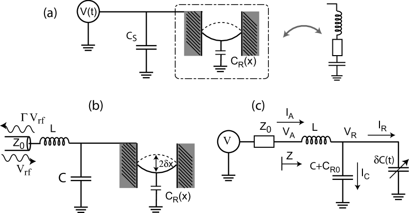
Figure 1: (a) Capacitive readout of a nanomechanical resonator (without a tank circuit) would suffer from the large parasitic wiring capacitances $C_{S}$. The drive $V(t)=V_{\mathrm{dc}}+V_{0}\cos(\omega_{0}t)$ is at mechanical resonance frequency $2\pi f_{0}$. Inset: electrical equivalent circuit how the mechanical resonator looks like at the same frequency as it is driven. (b) The signal is enhanced in our scheme by a low-$Q_{\mathrm{LC}}$ $LC$ tank circuit which blocks the stray capacitance. The vibrations of the beam (driven or not) at the mechanical frequency $f_{0}$ modulate the total capacitance of the tank circuit, and the signal occurs as sidebands of the reflected incoming wave $V_{\mathrm{r}f}\sin\left(\omega_{\mathrm{L}C}t\right)$ performed at the frequency $f_{\mathrm{L}C}\gg f_{0}$ of the tank circuit; (c) the circuit appears as one with a time-dependent capacitance when sensed at a frequency different from the actuation frequency $f_{0}$.

In Fig. 1 (a) we review our starting point, namely the idea of the capacitive actuation and readout, where the NR is driven by the voltage $V(t)=V_{\mathrm{dc}}+V_{0}\cos(\omega t)$. The NR oscillates as a Lorentzian about the (fundamental mode) mechanical resonance $\omega_{0}=2\pi f_{0}$:

$$\delta x(\omega,t)=\frac{F_{0}\cos(\omega t+\Theta)}{M\sqrt{\left(\omega\omega_{0}/Q_{M}\right)^{2}+\left(\omega^{2}-\omega_{0}^{2}\right)^{2}}}$$ (1)

where the driving ac-force is $F_{0}=\left(\frac{\partial C_{R}}{\partial x}\right)V_{\mathrm{dc}}V_{0}$, $\tan\Theta=\omega_{0}\omega\left[Q_{M}\left(\omega^{2}-\omega_{0}^{2}\right)\right]^{-1}$, $M$ is the effective mass of the fundamental mode (about 0.73 times the total mass of the beam), and $Q_{M}$ is the quality factor of the nanomechanical mode.

Equation (1) gives rise to a time-varying capacitance $C_{R}(t)=C_{R0}+\left(\frac{\partial C_{R}}{\partial x}\right)\delta x$, which at the drive frequency equals the electrical $RLC$ equivalent circuit shown in the inset of Fig. 1 (a).

On the mechanical resonance $\Theta=\pi/2$, current and voltage are in phase and and NR looks like a resistance. Towards increasing mechanical frequency, this effective resistance grows rapidly, and when combined with the large wiring stray capacitances $C_{S}$, makes the signal small. Truitt et al. Truitt et al. (2007) recently reported a progress which took advantage of the electrical analog augmented with a tank circuit in order to improve the impedance match to $Z_{0}=50\,\Omega$.

In order to analyze our approach, Fig. 1 (b), we write down the time-varying capacitance when the NR is resonantly actuated by $V(t)=V_{\mathrm{dc}}+V_{0}\cos(\omega_{0}t)$:

$$\begin{split}C_{R}=&C_{R0}+\delta x\left(\frac{\partial C_{R}}{\partial x}\right)\sin(\omega_{0}t)=\\ =&C_{R0}+\left(\frac{\partial C_{R}}{\partial x}\right)^{2}\frac{V_{\mathrm{dc}}V_{0}Q_{M}}{M\omega_{0}^{2}}\sin(\omega_{0}t)\end{split}$$ (2)

Here and henceforth, we will denote by $\delta x$ the resonant (maximum) value of the displacement in Eq. (1). We perform the measurement at a frequency $f_{\mathrm{LC}}$ fully different from the actuation frequency $f\sim f_{0}$, and as we shall see, this has the effect of erasing the phase relationship between the voltages and currents, and the NR therefore looks just like a time-varying capacitance, as displayed in Fig. 1 (c). At the measurement frequency $f_{\mathrm{LC}}$ the $RLC$ equivalent model still holds, but the impedance is such high that its contribution can be neglected. A related technique was recently demonstrated by Regal et al. Regal et al. (2008), however, they used a very high-$Q$ transmission line resonator as the coupling element, and a low-frequency NR.

For a more thorough analysis, let us write down the equations governing the flow of information between the different frequencies present in the problem, namely the actuation drive to the NR at the frequency $f_{0}$, measurement at $f_{\mathrm{LC}}=\frac{1}{2\pi\sqrt{L(C+C_{R0})}}$, and the mixing products (sidebands) $f_{\pm}\equiv f_{\mathrm{LC}}\pm f_{0}$, but neglecting higher-order mixing terms (a related analysis for the RF-SET can be found in Ref. Roschier et al. (2004)).

The voltages at the various frequencies in the middle of the tank circuit, at the point R in Fig. 1 (c) are, under these assumptions,

$$\begin{split}V^{R}&=V^{R}_{\mathrm{dc}}+V^{R}_{0}\exp\left(i\omega_{0}t\right)+V^{R}_{\mathrm{LC}}\exp\left(i\omega_{\mathrm{LC}}t\right)+\\ &V^{R}_{+}\exp\left[i(\omega_{\mathrm{LC}}+\omega_{0})t\right]+V^{R}_{-}\exp\left[i(\omega_{\mathrm{LC}}-\omega_{0})t\right]\end{split}$$ (3)

Using Eq. (2) for the time-dependent capacitance and Eq. (3) for the voltage across the NR, we get a relation for the currents $I^{R}$ flowing through the NR:

$$\begin{split}&I^{R}(t)=\frac{d}{dt}\left[C_{R}(t)V^{R}(t)\right]\simeq\\ &\frac{\delta x\left(\frac{\partial C_{R}}{\partial x}\right)}{2}\Huge\{\omega_{0}V^{R}_{\mathrm{dc}}\exp\left(i\omega_{0}t\right)+\omega_{\mathrm{LC}}(V^{R}_{+}-V^{R}_{-})\exp\left(i\omega_{\mathrm{LC}}t\right)\\ &+\omega_{+}V^{R}_{\mathrm{LC}}\exp\left(i\omega_{+}t\right)-\omega_{-}V^{R}_{\mathrm{LC}}\exp\left(i\omega_{-}t\right)\Huge\}+I_{R0}\end{split}$$ (4)

where $I_{R0}$ is the current through the constant part of the capacitance $C_{R0}$. We use the Kirchoff’s voltage and current laws which allow us to solve the circuit at all the mentioned three frequencies, when substituted by Eqs. (3,4):

$$\begin{split}V-I^{A}&\left(Z_{0}+i\omega L\right)-V^{R}=0\\ V^{R}=&\frac{I^{A}-I^{R}}{i\omega\left(C+C_{R0}\right)}\end{split}$$ (5)

If $\omega_{0}\ll\omega_{\mathrm{LC}}/Q_{\mathrm{LC}}$, and in the limit of small capacitance modulation $\delta x\left(\frac{\partial C_{R}}{\partial x}\right)\ll C_{R0}$, we obtain from Eqs. (5) the measured quantity, namely the voltage amplitudes $V_{\pm}=Z_{0}I^{A}_{\pm}$ of either sideband:

$$\begin{split}V_{+}=&V_{-}=\frac{\delta x\left(\frac{\partial C_{R}}{\partial x}\right)V_{\mathrm{rf}}}{2\omega_{\mathrm{LC}}(C+C_{R0})^{2}Z_{0}}=\\ \simeq&\left(\frac{C_{R0}}{C+C_{R0}}\right)^{2}\frac{Q_{M}V_{\mathrm{dc}}V_{0}V_{\mathrm{rf}}}{2x_{0}^{2}M\omega_{\mathrm{LC}}Z_{0}\omega_{0}^{2}}\end{split}$$ (6)

where for the last form, we substituted the capacitance modulation amplitude $\delta C$ as defined in Eq. (2), and then approximated it as $\frac{\partial C_{R}}{\partial x}\sim\frac{C_{R0}}{x_{0}}$ where $x_{0}$ is the vacuum gap between the beam and the gate. As one would intuitively think, the signal depends strongly on how much stray capacitance $C$ one has within the resonant circuit, the part which is not cancelled by the inductor. The signal is proportional to both actuation parameters ($V_{\mathrm{d}c}$ and $V_{0}$) and to how much the system responds, given by $Q_{M}$, as well as to the measurement strength $V_{\mathrm{r}f}$. Also, the signal can be interpreted as being proportional to the quality factor $Q_{\mathrm{L}C}\sim\left(\omega_{\mathrm{L}C}CZ_{0}\right)^{-1}$ of the tank circuit. The bandwidth, as typical of a modulation scheme, is given by the response time of the electrical tank circuit, as $f_{\mathrm{L}C}/Q_{\mathrm{L}C}$.

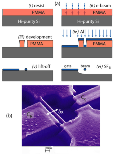
Figure 2: The fabrication of the nanomechanical resonators on high-resistivity Silicon substrate; (a) the process steps: (i) high-purity Si substrate is coated by 300 nm of PMMA resist; (ii) positive e-beam exposure of the final pattern; (iii) resist development; (iv) e-beam evaporation of a thickness $h=50$ nm or $h=100$ nm of Aluminum; (v) lift-off in acetone; (vi) the chip as a whole is exposed to SF₆ Reactive Ion Etch (RIE) which removes $\sim 1\,\mu$m layer of the Si substrate. (b) SEM image of a $l=1.8\,\mu$m long and $W=160$ nm wide Al beam (similar to samples A and B). The scale bar is 200 nm. The beam is driven to oscillate (amplitude $\delta x$) in the plane of the film due to capacitive drive from the large gate $C_{R}$. The same gate is also used to sense the motion. The other, weakly coupled, gate $C_{g}$ was not used presently.

For the fabrication of micron-scale suspended, metallized of fully metallic nanomechanical beams, a multitude of ingenious methods have been developed Cleland and Roukes (1996); Cleland et al. (2001); Yang et al. (2001); Husain et al. (2003); Sekaric et al. (2002); Sazonova et al. (2004); Li et al. (2008). Our process represents the simplest end of the spectrum in terms of the complexity of the process, and the number of steps needed. The beam itself is metallic, and hence there is no separate metallization needed. The fabrication goes on top of a high-resistivity ($\sim 3$ k$\Omega$m) Silicon as shown in Fig. 2, by e-beam lithography. In the end, a properly timed SF₆ dry etch suspends the beam, while leaving the clamps in both ends well hooked to the substrate.

For the measurements, the chip was wire-bonded to a surface-mount inductor $L=10...30$ nH in a sample holder. The tank circuit capacitance $C\sim 0.3$ pF comes from the stray capacitances of the bonding pad and of the inductor. The choice of the inductor was made such that the expected mechanical frequency falls within the electrical bandwidth $Z_{0}/(2\pi L)$. The sample was connected to high-frequency coaxial cables in a test cryostat, and cooled down to 4 K in a vacuum of $\sim 10^{-2}$ mBar. The voltages at dc, at the NR drive frequency, and at the measurement frequency were combined at room temperature using bias tees. The signal reflected from the sample was feed to a spectrum analyzer via a circulator and room temperature microwave amplifiers having the noise temperature $T_{N}\sim 100$ K which set the noise level in the measurement. The driven mechanical response was obtained by scanning the drive frequency $f_{g}$ about the mechanical resonance $f_{0}$, and recording the amplitude of the sideband voltage.

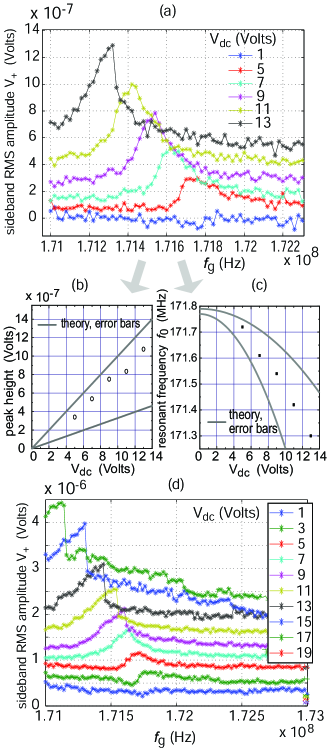
Figure 4: As Fig. 3; measurement and analysis for sample A; (a) $V_{0}=50$ mV and probe $V_{\mathrm{LC}}=140$ mV, for increasing values of the dc voltage $V_{\mathrm{dc}}$ from bottom to top (displaced vertically for clarity); (b) increase of the height of the peak versus dc voltage; (c) frequency shift versus dc voltage; (d) at a higher total drive $V_{0}=50$ mV and $V_{\mathrm{LC}}=200$ mV, the system turns nonlinear and hysteretic.

We studied a total of four samples as summarized in Table 1 for their dimensions, the used tank circuit, and the basic characteristics $f_{0}$ and $Q_{M}$ of the resonance. In Figs. 3, 4 we show more data for two representative samples.

Table 1: List of the measured nanomechanical resonators. They were fabricated out of Al according to Fig. 2. Sample C was baked in vacuum at 200^oC for 15 min. The quality factors $Q_{M}$ and the fundamental mode resonance frequencies $f_{0}$ were measured in a temperature of 4.2 K in a vacuum of $\sim 10^{-2}$ mBar. The estimated frequency is given as $f_{0}\simeq\frac{W}{l^{2}}\sqrt{\frac{E}{\rho}}$, where $E$ is the Young modulus and $\rho$ is density. The other beam parameters are $l=$length, $W$ = width, $h$ = thickness, $x_{0}$ = vacuum gap.

sample	$l$	$W$	$h$	$x_{0}$	$f_{0}$ (est)	$f_{0}$ (meas)	$L$	$C_{R}$	$C$	$f_{\mathrm{LC}}$	$Q_{M}$
A	1.8 $\mu$m	150 nm	100 nm	65 nm	230 MHz	172 MHz	20 nH	47 aF	0.39 pF	1.81 GHz	$1.0\times 10^{3}$
B	1.8 $\mu$m	160 nm	50 nm	70 nm	245 MHz	191 MHz	14 nH	45 aF	0.27 pF	2.16 GHz	$1.0\times 10^{3}$
C	2.2 $\mu$m	200 nm	75 nm	100 nm	205 MHz	202 MHz	10 nH	64 aF	0.3 pF	3.02 GHz	$1.0\times 10^{3}$
D	2.5 $\mu$m	145 nm	150 nm	170 nm	117 MHz	130 MHz	10 nH	49 aF	0.3 pF	2.95 GHz	$2.6\times 10^{3}$

As the basic test of the scheme, we compared the measured sideband voltage to that expected, Eq. (6) according to our model of a time-varying capacitance. We model the capacitance $C_{R}$ between the beam and the nearby gate as that for two parallel beams of length $l$, width $W$ and a vacuum gap $x_{0}$:

$$C_{R}(x_{0})=\pi\epsilon_{0}l\left\{\ln\left[\frac{x_{0}}{W}+1+\sqrt{\left(\frac{x_{0}}{W}\right)^{2}+\frac{2x_{0}}{W}}\right]\right\}^{-1}$$ (7)

In Figs. 3 (b), 4 (b) we plot the height of the peak obtained as the drive frequency $f_{g}$ was scanned through the resonance, as a function of the dc voltage. We calculate numerically $\left(\frac{\partial C_{R}}{\partial x}\right)$ which we use in Eq. (6) in order to obtain the gray lines illustrating the expected linear increase of the peak height, showing a good agreement with the data. The error bars arise from uncertainties in the attenuation of the system at low temperature, as well as uncertainty in the exact value of the beam gap $x_{0}$ to which the capacitance is sensitive. Note, however, that all the parameters were independently estimated.

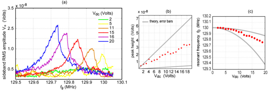
Figure 3: Measurements of the response of the nanomechanical resonator (sample D) using the electric sideband detection, $V_{0}=100$ mV and $V_{\mathrm{LC}}=30$ mV, at $T=4.2$ K; (a) resonance curves of the fundamental mode for increasing dc voltage (from right to left); (b) Amplitude of the peak extracted from (a). The theoretical predictions (gray lines) are scaled down by the total microwave attenuation $\sim 10$ dB of the system; (c) center frequency of the mechanical peak extracted from (a), compared to theory from Eq. (8);

As a further test of integrity of our model, we studied the shift of the linear-regime resonant frequency as a function of the applied dc voltage $V_{\mathrm{dc}}$. Due to electrostatic softening of the effective spring constant $k^{*}(V_{\mathrm{dc}})=k-\frac{1}{2}V_{\mathrm{d}c}^{2}\frac{\partial^{2}C_{R}}{\partial x^{2}}\Large|_{V_{\mathrm{dc}}}$, the resonance is expected to shift left with increasing dc voltage:

$$\omega_{0}\left(V_{\mathrm{dc}}\right)=\omega_{0}\left(0\right)\left[1-\frac{C_{R0}V_{\mathrm{dc}}^{2}}{2M\omega_{0}^{2}\left(0\right)x_{0}^{2}}\right]$$ (8)

which holds well for the gap smaller than beam diameter. In Figs. 3 (c), 4 (c) we plot the theory prediction together with data as the gray curves which represent Eq. (8) evaluated at opposite limits of the error bars. We notice the match is good to both the magnitude of the frequency shift, as well as its expected quadratic behavior, again without any fitting parameters.

The mechanical frequencies summarized in Table 1 agree within 25 % of the prediction based on a stress-free film. For samples A and B the measured frequency falls below the predicted, whereas C and D show the opposite. Sample C was briefly heat-treated (see Table 1), which could have removed the supposedly compressive stress present in the film after evaporation, thus causing the frequency to go up. The good mechanical $Q$-values $Q_{M}>10^{3}$, in agreement with previous 4-Kelvin experiments on Aluminum beams Li et al. (2008), do not indicate damage to the beam material was caused by the process.

While our scheme in principle offers room temperature operation, we found out that the (small) conductivity of the Si substrate caused spurious non-linearities at temperatures above that of liquid nitrogen (77 K), which masked the signal. This issue could be settled by using a more resistive substrate, such as oxidized Silicon.

The fast sideband detection procedure which we demonstrate here offers a sensitive, an in-principle tabletop characterization method for the nanomechanical resonators. A major figure of merit is the displacement sensitivity $s_{x}$. It is obtained from Eq. (6) as the value of $\delta x$ which would correspond to a voltage spectral density equal to the noise voltage $\sqrt{2k_{B}T_{N}Z_{0}}$ which we suppose is set by the amplifiers:

$$s_{x}\simeq 2\sqrt{2k_{B}T_{N}Z_{0}^{3}}x_{0}\frac{\omega_{\mathrm{LC}}(C+C_{R0})^{2}}{C_{R0}V_{\mathrm{rf}}}$$ (9)

where $T_{N}$ is the noise temperature of the system. Notice that the sensitivity does not depend on the actuation voltages $V_{\mathrm{d}c}$ and $V_{0}$, but evidently improves with increasing measurement voltage $V_{\mathrm{r}f}$ under the assumption that linearity holds. The dependence on the sample dimensions comes via $C_{R0}$ which scales with the length $l$ as $C_{R0}\propto l$. Hence in the ”easy” limit where the stray capacitance $C$ dominates, towards small size the sensitivity degrades relatively slowly, as $\propto l^{-2}$. For instance, we expect the method to be usable in order to detect small vibrations for an Al doubly clamped beam of length $l=0.7\,\mu$m, $f_{0}\simeq 1$ GHz. Let us use the moderate values $L=8$ nH, $C=0.1$ pF, $T_{N}=100$ K, $V_{\mathrm{rf}}=3$ mV, and $V_{\mathrm{dc}}=10$ V, with which values we find a sensitivity of $s_{x}\sim 0.5$ pm$/\sqrt{\mathrm{Hz}}$.

The sideband readout also seems promising for basic studies of the NR at low temperatures, since the NR and its surroundings stay superconducting. The dispersive detection where only the phase of the reflected signal varies, as well as the all-electric actuation we apply, cause a vanishing on-chip dissipation.

Interestingly, the sideband measurement might also offer a path towards the quantum limit of mechanical motion. Through minimization of the tank circuit capacitance $C$ in Fig. 1 (b) by improving the $LC$ tank circuit from our first realization made of surface mount components, one could approach the sensitivity needed for observing the mechanical zero-point vibrations. The lowest $C$ would be achieved by fabricating the NR coupled to an on-chip spiral coil, for example $L=17$ nH, $C\sim 25$ fF. Let us consider an Aluminum beam having a length $l=1.5\,\mu$m and frequency $f_{0}=240$ MHz. Let us also take $f_{\mathrm{L}C}=5$ GHz and $T_{N}=4$ K. If probed even with a decent $V_{\mathrm{rf}}=3$ mV, and $V_{\mathrm{dc}}=10$ V, Eq. (9) yields a displacement sensitivity $s_{x}\sim 45$ fm$/\sqrt{\mathrm{Hz}}$, which comes interestingly close to the zero-point aplitude $x_{\mathrm{zp}}\sim 25$ fm whose energy will be spread over a bandwidth determined by $Q_{M}$. The back-action disturbance due to the probing remains small, since $f_{\mathrm{LC}}\gg f_{0}$. The back-action is estimated from the tail of the Lorentzian response of Eq. (1), where the amplitude at high frequencies decays as $\left(f_{\mathrm{LC}}\right)^{-3}$. With the above parameter values, we find that the measurement would excite less than one quantum of energy into the NR.

An interesting materials platform for the sideband readout, among all conductive materials, is graphene Bunch et al. (2007). The signal improves due to a large capacitance of the sheet and due to its low mass, whereas the latter also substantially increases the zero-point amplitude. Due to the sensitivity of the novel method, interesting mass, acceleration or other sensor applications might also arise.

References

- Cleland (2003) A. Cleland, Foundations of Nanomechanics (Springer, New York, 2003).
- Ekinci and Roukes (2005) K. L. Ekinci and M. L. Roukes, Rev. Sci. Instrum. 76, 061101 (2005).
- Jensen et al. (2008) K. Jensen, K. Kim, and A. Zettl, Nature Nanotech. 3, 533 (2008).
- Irish and Schwab (2003) E. K. Irish and K. Schwab, Phys. Rev. B 68, 155311 (2003).
- Cleland and Geller (2004) A. N. Cleland and M. R. Geller, Phys. Rev. Lett. 93, 070501 (2004).
- Greywall et al. (1994) D. S. Greywall, B. Yurke, P. A. Busch, A. N. Pargellis, and R. L. Willett, Phys. Rev. Lett. 72, 2992 (1994).
- Cleland and Roukes (1996) A. N. Cleland and M. L. Roukes, Appl. Phys. Lett. 69, 2653 (1996).
- Ekinci et al. (2002) K. L. Ekinci, Y. T. Yang, X. M. H. Huang, and M. L. Roukes, Appl. Phys. Lett. 81, 2253 (2002).
- Li et al. (2008) T. F. Li, Y. A. Pashkin, O. Astafiev, Y. Nakamura, J. S. Tsai, and H. Im, Appl. Phys. Lett. 92, 043112 (2008).
- LaHaye et al. (2004) M. D. LaHaye, O. Buu, B. Camarota, and K. C. Schwab, Science 304, 74 (2004).
- Naik et al. (2006) A. Naik, O. Buu, M. D. LaHaye, A. D. Armour, A. A. Clerk, M. P. Blencowe, and K. C. Schwab, Nature 443, 193 (2006).
- Regal et al. (2008) J. D. Regal, C. A. Teufel, and K. W. Lehnert, Nature Physics 4, 555 (2008).
- Huang et al. (2003) X. M. H. Huang, C. A. Zorman, M. Mehregany, and M. L. Roukes, Nature 421, 496 (2003).
- Truitt et al. (2007) P. A. Truitt, J. B. Hertzberg, C. C. Huang, K. L. Ekinci, and K. C. Schwab, Nano Lett. 7, 120 (2007).
- Schoelkopf et al. (1998) R. Schoelkopf, P. Wahlgren, A. Kozhevnikov, P. Delsing, and D. Prober, Science 280, 1238 (1998).
- Roschier et al. (2005) L. Roschier, M. Sillanpää, and P. Hakonen, Phys. Rev. B 71, 024530 (2005).
- Sillanpää et al. (2004) M. Sillanpää, L. Roschier, and P. Hakonen, Phys. Rev. Lett. 93, 066805 (2004).
- Roschier et al. (2004) L. Roschier, M. Sillanpää, T. Wang, M. Ahlskog, S. Iijima, and P. Hakonen, Journal of Low Temperature Physics 136, 465 (2004).
- Cleland et al. (2001) A. N. Cleland, M. Pophristic, and I. Ferguson, Appl. Phys. Lett. 79, 2070 (2001).
- Yang et al. (2001) Y. T. Yang, K. L. Ekinci, X. M. H. Huang, L. M. Schiavone, M. L. Roukes, C. A. Zorman, and M. Mehregany, Appl. Phys. Lett. 78, 162 (2001).
- Husain et al. (2003) A. Husain, J. Hone, H. W. C. Postma, X. M. H. Huang, T. Drake, M. Barbic, A. Scherer, and M. L. Roukes, Appl. Phys. Lett. 83, 1240 (2003).
- Sekaric et al. (2002) L. Sekaric, J. M. Parpia, H. G. Craighead, T. Feygelson, B. H. Houston, and J. E. Butler, Appl. Phys. Lett. 81, 4455 (2002).
- Sazonova et al. (2004) V. Sazonova, Y. Yaish, T. A. H. Üstünel, D. Roundy, and P. McEuen, Nature 431, 284 (2004).
- Bunch et al. (2007) J. S. Bunch, A. M. van der Zande, S. S. Verbridge, I. W. Frank, D. M. Tanenbaum, J. M. Parpia, H. G. Craighead, and P. L. McEuen, Science 315, 490 (2007).