Finite-matrix formulation of gauge theories
on a non-commutative torus
with twisted boundary conditions

Abstract:

We present a novel finite-matrix formulation of gauge theories on a non-commutative torus. Unlike the previous formulation based on a map from a square matrix to a field on a discretized torus with periodic boundary conditions, our formulation is based on the algebraic characterization of the configuration space. This enables us to describe the twisted boundary conditions in terms of finite matrices and hence to realize the Morita equivalence at a fully regularized level. Matter fields in the fundamental representation turn out to be represented by rectangular matrices for twisted boundary conditions analogously to the matrix spherical harmonics on the fuzzy sphere with the monopole background. The corresponding Ginsparg-Wilson Dirac operator defines an index, which can be used to classify gauge field configurations into topological sectors. We also perform Monte Carlo calculations for the index as a consistency check. Our formulation is expected to be useful for applications of non-commutative geometry to various problems related to topological aspects of field theories and string theories.

1 Introduction

Non-commutative (NC) geometry [1, 2] was proposed long time ago as a simple modification of our notion of space-time at short distances possibly due to effects of quantum gravity [3]. It has attracted much attention since field theories on a NC geometry were shown to appear naturally from matrix models [4, 5] and from string theories [6]. In fact it turned out that the NC geometry affects not only the short-distance physics but also the long-distance physics through loop effects. This UV/IR mixing phenomenon [7] makes such field theories more interesting due to rich physics, but it also poses both technical and conceptual problems in various applications. In particular, the appearance of a new type of IR divergence spoils the perturbative renormalizability in most cases [8]. Therefore, nonperturbative studies of NC field theories based on a suitable regularization are highly motivated.

Not surprisingly, considering the links to string theory, a natural regularization of NC field theories is possible by representing fields by finite matrices. In the case of a NC torus, for instance, the so-called twisted Eguchi-Kawai model [9, 10] is reinterpreted as a lattice formulation of NC field theories [11], in which a finite $N$ matrix is mapped one-to-one onto a field on a discretized torus. Monte Carlo simulations based on this formulation have been performed intensively. For instance, in ref. [12] the existence of a sensible continuum limit (and hence the nonperturbative renormalizability) of a NC field theory was shown for the first time in the case of U(1) gauge theory on a 2d NC torus. Spontaneous breaking of the translational symmetry [13, 14, 15], which occurs as a result of the UV/IR mixing effects, has been studied nonperturbatively in NC scalar field theories [16, 17] and in NC U(1) gauge theory in 4d [18]. This phenomenon may be viewed as the collapsing of the NC manifolds [19, 20].

Another interesting feature of NC field theories is the appearance of a new type of topological objects [21]. We consider it important to study dynamical properties of these objects, since they may play an important role in physical problems such as the strong CP problem and the baryon number non-conservation in the electroweak theory, which are expected to be related to topological aspects of field theories. They may also be relevant to string theory, in which chiral fermions on our space-time are considered to be realized by compactification with a nontrivial index in the extra dimensions. In order to address such dynamical issues, we need to perform nonperturbative studies based on a regularized formulation. It turned out, however, that finite-matrix description of topologically nontrivial configurations is not that straightforward. For instance, refs. [22, 23] use mathematical devices such as the projective modules and the algebraic K-theory.

The difficulty is related to the fact that topologically nontrivial configurations in the commutative space typically allow two descriptions; one in terms of single-valued functions with singularities, and the other in terms of multi-valued functions without singularities. These two descriptions are related to each other through a singular gauge transformation. In the case of NC geometry the first description is somehow prohibited due to smearing effects. This is demonstrated on a NC torus with periodic boundary conditions [24, 25, 26], where topologically nontrivial configurations are shown to be suppressed in the continuum limit. The situation is in sharp contrast to that in the commutative space as seen in lattice simulations [28]. Thus we are led to consider the second description.

As in the commutative case, one can think of twisting boundary conditions [29], which corresponds to introducing a background magnetic flux. However, the finite-matrix formulation of gauge theories on a NC torus proposed in ref. [11] essentially deals with the case of periodic boundary conditions. In this paper we reconsider the formulation from a purely algebraic point of view, and generalize it in such a way that it allows for explicit description of twisted boundary conditions in terms of finite matrices. Our new formulation realizes the Morita equivalence at a fully regularized level. Matter fields in the fundamental representation can be naturally described by finite rectangular matrices in the presence of the magnetic flux. This is analogous to the situation in the fuzzy sphere case with the monopole background, where rectangular matrices appear as the matrix version of the monopole harmonics [23, 31, 32]. The corresponding Ginsparg-Wilson Dirac operator enables us to define an index, which can be used to classify regularized gauge field configurations into topological sectors. We present Monte Carlo results for the index, which demonstrate that topologically nontrivial configurations indeed survive the continuum limit in a 2d gauge theory with twisted boundary conditions.

In fact there is yet another possibility for realizing topologically nontrivial configurations, in which they are described by both single-valued and regular functions. The idea is to consider the Higgs phase of gauge theories, where the winding number of the Higgs field substitutes the role of the twisted boundary conditions. While we do not discuss this possibility in this paper, let us comment on some recent developments in this direction. In the case of fuzzy sphere, the corresponding finite-matrix formulation was constructed, and the index of the Ginsparg-Wilson Dirac operator involving the Higgs field, which reproduces the Higgs winding number, was formulated for general background configurations [31, 27]. An explicit NC configuration corresponding to the ’t Hooft-Polyakov monopole was constructed [23, 34], and the spectrum of matter fluctuations around this background was obtained [23, 31]. The matrix version of monopole harmonics, which appears here, plays an important role also in a nonperturbative formulation of super Yang-Mills theory on $R\times S^{3}$, where $S^{3}$ is regarded as an $S^{1}$ bundle over $S^{2}$ [35]. We expect that the ideas to use regular configurations for describing nontrivial topological sectors in NC geometry by considering the winding Higgs field or the twisted boundary conditions, provide physical understanding to the previous mathematical formulations [22, 23] mentioned above.

The rest of this paper is organized as follows. In section 2 we briefly review the gauge theories on a NC torus with twisted boundary conditions. A more detailed review is provided in appendix A. In section 3 we rewrite the boundary conditions in a covariant form. In section 4 we characterize the configuration space of a regularized field as a representation space of the algebra of the coordinate and shift operators. In section 5 we explicitly construct the representation space of the algebra to arrive at a finite-matrix formulation for twisted boundary conditions. In section 6 we describe the actions for the gauge field and for fundamental matters. In section 7 we present Monte Carlo results for the index of the Ginsparg-Wilson Dirac operator. Section 8 is devoted to a summary and discussions.

2 Brief review of gauge theories on a NC torus

In this section we briefly review gauge theories on a continuous NC torus with twisted boundary conditions, which form the basis of our finite-matrix formulation. The readers who are not familiar with the subject are recommended to read appendix A, where we provide a more detailed and self-contained review. There one can also find some derivations omitted in this section, descriptions in terms of fields instead of operators, and an explicit form of the actions.

In NC geometry the coordinate operators $\hat{x}_{\mu}$ and the derivative operators $\hat{\partial}_{\mu}$ satisfy the algebra

$$\left[\hat{x}_{\mu}\,,\,\hat{x}_{\nu}\right]=i\,\theta_{\mu\nu}~{},~{}~{}\left[\hat{\partial}_{\mu}\,,\,\hat{x}_{\nu}\right]=\delta_{\mu\nu}~{},~{}~{}$$ (1)

where $\theta_{\mu\nu}$ represents the non-commutativity of the space-time. Let us consider a $D$-dimensional torus with the period $L$. When we impose periodic boundary conditions, we consider the operators $\hat{Z}_{\mu}=e^{2\pi i\hat{x}_{\mu}/L}$ instead of $\hat{x}_{\mu}$, and the algebra (1) becomes

$$\hat{Z}_{\mu}\hat{Z}_{\nu} = e^{-2\pi i\Theta_{\mu\nu}}\hat{Z}_{\nu}\hat{Z}_{\mu}\ ,$$ (2)

$$\left[\hat{\partial}_{\mu},\ \hat{Z}_{\nu}\right] = 2\pi i\frac{1}{L}\delta_{\mu\nu}\hat{Z}_{\nu}\ ,$$ (3)

where $\Theta_{\mu\nu}=\frac{2\pi}{L^{2}}\theta_{\mu\nu}$. For the purpose that will be clear later, we impose the commutation relation

$$\left[\hat{\partial}_{\mu}\,,\,\hat{\partial}_{\nu}\right]=-i\,c_{\mu\nu}$$ (4)

on the derivative operator $\hat{\partial}_{\mu}$. Here the real anti-symmetric tensor $c_{\mu\nu}$ is left arbitrary at this point, since the derivative operator $\hat{\partial}_{\mu}$ acts on fields (or functions of the coordinate operators) as adjoint, and the parameter $c_{\mu\nu}$ does not affect the commutativity of an action of $\hat{\partial}_{\mu}$ on to the field $\Phi$ since $[\hat{\partial}_{\mu},[\hat{\partial}_{\nu},\Phi]]=[\hat{\partial}_{\nu},[\hat{\partial}_{\mu},\Phi]]$ due to the Jacobi identity.

When we impose twisted boundary conditions on a U($p$) gauge field, it is convenient to think of a constant-curvature U(1) background field $\hat{A}^{(0)}_{\mu}$, which obeys the boundary conditions. Defining the covariant derivative for the background as

$$\hat{D}^{(0)}_{\mu}=\hat{\partial}_{\mu}-i\hat{A}^{(0)}_{\mu}\ ,$$ (5)

the background flux is given by

$$f_{\mu\nu}=i\left[\hat{D}_{\mu}^{(0)},\hat{D}_{\nu}^{(0)}\right]-i\left[\hat{\partial}_{\mu}\,,\,\hat{\partial}_{\nu}\right]\ .$$ (6)

We decompose the gauge field into the background and the fluctuation as

$$\hat{A}_{\mu}=\hat{A}^{(0)}_{\mu}+\hat{{\cal A}}_{\mu}\ ,$$ (7)

so that the boundary conditions for $\hat{{\cal A}}_{\mu}$ take the homogeneous form

$${\,\rm e}\,^{L\hat{\partial}_{\nu}}~{}\hat{\cal A}_{\mu}~{}{\,\rm e}\,^{-L\hat{\partial}_{\nu}}=\hat{\Omega}_{\nu}~{}\hat{\cal A}_{\mu}~{}\hat{\Omega}_{\nu}^{\dagger}\ .$$ (8)

The transition functions $\hat{\Omega}_{\mu}$ are chosen as

$$\hat{\Omega}_{\mu}={\,\rm e}\,^{i\alpha_{\mu\nu}\hat{x}_{\nu}}\otimes\Gamma_{\mu}^{(p)}\ ,$$ (9)

where $\alpha_{\mu\nu}$ are constant real values and $\Gamma^{(p)}_{\mu}$ are constant SU($p$) matrices. The fact that the background field $\hat{A}^{(0)}_{\mu}$ obeys the boundary conditions fixes $\alpha_{\mu\nu}$. The so-called co-cycle condition (105), which represents the consistency of the boundary conditions, requires $\Gamma^{(p)}_{\mu}$ to satisfy the ’t Hooft-Weyl algebra. In the 2d case, for instance, it is given as

$$\Gamma^{(p)}_{\mu}\Gamma^{(p)}_{\nu}=e^{-2\pi i\varepsilon_{\mu\nu}\frac{q}{p}}\Gamma^{(p)}_{\nu}\Gamma^{(p)}_{\mu}\ ,$$ (10)

where $\varepsilon_{\mu\nu}$ is an anti-symmetric tensor with $\varepsilon_{12}=1$. Then the co-cycle condition (105) further requires the background abelian flux $f_{12}$ to be given by

$$f_{12}\equiv F=\frac{2\pi q}{L^{2}(p-\Theta q)}\ ,$$ (11)

where $\Theta_{\mu\nu}=\Theta\varepsilon_{\mu\nu}$. Solving this for the integer $q$, we obtain

$$q=\frac{1}{2\pi}\frac{FL^{2}}{1+\theta F}p\ ,$$ (12)

where $\theta_{\mu\nu}=\theta\varepsilon_{\mu\nu}$.

The surprising fact about NC geometry is that the above gauge theory can be mapped to a gauge theory on a dual NC torus with periodic boundary conditions. This can be demonstrated by showing that the general solution to (8) is given, for instance, in 2d by (See section A.3.)

$$\hat{\cal A}_{\mu}=\sum_{\vec{m}\in\mathbb{Z}^{2}}\,\prod_{\nu=1}^{2}\left(\hat{Z}^{\prime}_{\nu}\right)^{m_{\nu}}\,\prod_{\lambda<\rho}{\,\rm e}\,^{-\pi i\,m_{\lambda}\,\Theta^{\prime}_{\lambda\rho}\,m_{\rho}}\,\cdot\Bigl{(}{1\!\!1}\otimes a_{\mu}(\vec{m})\Bigr{)}\ ,$$ (13)

where $a_{\mu}(\vec{m})$ are $p_{0}\times p_{0}$ matrices with $p_{0}$ being the greatest common divisor of $p$ and $q$. Let us introduce integers $\tilde{p}$ and $\tilde{q}$ by

$$p=p_{0}\,\tilde{p}\ ,\ \ q=p_{0}\,\tilde{q}\ .$$ (14)

Since $\tilde{p}$ and $\tilde{q}$ are co-prime, the integers $a$ and $b$ in the Diophantine equation

$$a\tilde{p}+b\tilde{q}=1$$ (15)

are uniquely determined up to the shift $(a,b)\sim(a,b)+(\tilde{q},-\tilde{p})$. The operators $\hat{Z}^{\prime}_{\mu}$ in (13) are written in the form

$$\hat{Z}^{\prime}_{\mu}={\,\rm e}\,^{2\pi i\beta_{\nu\mu}\hat{x}_{\nu}}\otimes\prod_{\nu=1}^{2}(\Gamma^{(p)}_{\nu})^{b\varepsilon_{\nu\mu}}\ ,$$ (16)

where $\beta_{\nu\mu}$ is given by (123), and $b$ is the integer appearing in (15). One can also show that the operators $\hat{Z}^{\prime}_{\mu}$ and $\hat{D}^{(0)}_{\mu}$ satisfy the commutation relations

$$\hat{Z}^{\prime}_{\mu}\,\hat{Z}^{\prime}_{\nu} = {\,\rm e}\,^{-2\pi i\,\Theta^{\prime}\varepsilon_{\mu\nu}}\,\hat{Z}^{\prime}_{\nu}\,\hat{Z}^{\prime}_{\mu}\ ,$$ (17)

$$\left[\hat{D}^{(0)}_{\mu}\,,\,\hat{Z}^{\prime}_{\nu}\right] = 2\pi i\,L^{\prime-1}\delta_{\mu\nu}\,\hat{Z}^{\prime}_{\nu}\ ,$$ (18)

$$\left[\hat{D}_{\mu}^{(0)},\hat{D}_{\nu}^{(0)}\right] = -i(c_{\mu\nu}+f_{\mu\nu})\ ,$$ (19)

where the parameters $\Theta^{\prime}$ and $L^{\prime}$ are given by

$$\Theta^{\prime} = \frac{a\Theta+b}{\tilde{p}-\tilde{q}\Theta}\,\ ,$$ (20)

$$L^{\prime} = L\,(\tilde{p}-\Theta\tilde{q})\ .$$ (21)

The algebra (17)-(19) have the same form as (2)-(4) for the periodic boundary conditions. This implies that the U($p$) gauge theory with twisted boundary conditions on a NC torus characterized by $\Theta$ and $L$ can be mapped to a dual U($p_{0}$) gauge theory with periodic boundary conditions on a NC torus characterized by $\Theta^{\prime}$ and $L^{\prime}$. The covariant derivative operator $\hat{D}^{(0)}_{\mu}$ on the original torus plays the role of the derivative operator $\hat{\partial}^{\prime}_{\mu}$ on the dual torus. This equivalence of the two NC theories is known as the Morita equivalence.

When the theory includes only fields in the adjoint representation, which obey the boundary conditions

$${\,\rm e}\,^{L\hat{\partial}_{\nu}}~{}\hat{\Phi}~{}{\,\rm e}\,^{-L\hat{\partial}_{\nu}}=\hat{\Omega}_{\nu}~{}\hat{\Phi}~{}\hat{\Omega}_{\nu}^{\dagger}\ ,$$ (22)

one can map them to fields in the dual theory with periodic boundary conditions as we did above for the gauge field. Using a map from finite matrices to fields on a discretized NC torus with periodic boundary conditions, one can indirectly regularize the original theory with twisted boundary conditions [11]. However, the Morita equivalence does not hold in general for theories including matter fields in the fundamental representation, which obey the boundary conditions

$${\,\rm e}\,^{L\hat{\partial}_{\nu}}~{}\hat{\Phi}~{}{\,\rm e}\,^{-L\hat{\partial}_{\nu}}=\hat{\Omega}_{\nu}~{}\hat{\Phi}\ .$$ (23)

These conditions can be solved explicitly [36], but the obtained solution does not suggest any obvious way to regularize the theory unlike the situation with the adjoint matters. Our idea is therefore to construct the configuration space of a regularized field in a purely algebraic way.

3 Rewriting boundary conditions in a covariant form

The gauge invariance of NC gauge theories is represented by SU($N$) symmetry in the finite-$N$ matrix formulation. Therefore our important first step is to rewrite the boundary conditions (22) and (23) in a gauge-covariant form.

In this section, by gauge covariance we mean the covariance under the transformation of the gauge field (7)

$$\hat{A}_{\mu}\to\hat{g}\,\hat{A}_{\mu}\,\hat{g}^{\dagger}+i\,\hat{g}\,[\hat{\partial}_{\mu},\,\hat{g}^{\dagger}]\ ,$$ (24)

together with the same one for the background field

$$\hat{A}_{\mu}^{(0)}\to\hat{g}\,\hat{A}_{\mu}^{(0)}\,\hat{g}^{\dagger}+i\,\hat{g}\,[\hat{\partial}_{\mu},\,\hat{g}^{\dagger}]\ ,$$ (25)

so that the covariant derivative operator $\hat{D}^{(0)}_{\mu}$ given by (5) and the fluctuation part $\hat{\cal A}_{\mu}$ transform covariantly as

$$\hat{D}^{(0)}_{\mu} \to \hat{g}\,\hat{D}^{(0)}_{\mu}\,\hat{g}^{\dagger}\ ,$$

$$\hat{\cal A}_{\mu} \to \hat{g}\,\hat{\cal A}_{\mu}\,\hat{g}^{\dagger}\ .$$ (26)

This motivates us to rewrite the twisted boundary conditions (8) as

$$e^{L\hat{D}^{(0)}_{\nu}}\,\hat{\cal A}_{\mu}\,e^{-L\hat{D}^{(0)}_{\nu}}=\hat{\Xi}_{\nu}\,\hat{\cal A}_{\mu}\,\hat{\Xi}_{\nu}^{\dagger}\ ,$$ (27)

where we have defined the operator

$$\hat{\Xi}_{\mu}=e^{L\hat{D}^{(0)}_{\mu}}e^{-L\hat{\partial}_{\mu}}\hat{\Omega}_{\mu}\ ,$$ (28)

which transforms covariantly as

$$\hat{\Xi}_{\mu}\to\hat{g}\,\hat{\Xi}_{\mu}\,\hat{g}^{\dagger}\ .$$ (29)

The key observation for our formulation is that actually $\hat{\Xi}_{\mu}$ can be written in terms of the coordinate operators $\hat{Z}_{\mu}^{\prime}$ of the dual torus that appear in (13). In 2d, for instance, $\hat{\Xi}_{\mu}$ and $\hat{Z}_{\mu}^{\prime}$ are given explicitly as (117) and (124). Using (12) and (15), one can easily show that

$$\hat{\Xi}_{1}=(\hat{Z}^{\prime}_{2})^{\tilde{q}}\quad,\quad\hat{\Xi}_{2}=(\hat{Z}^{\prime}_{1})^{-\tilde{q}}\ .$$ (30)

Although the above relation was obtained in the specific gauge (113), it should hold gauge independently since both $\hat{\Xi}_{\mu}$ and $\hat{Z}^{\prime}_{\mu}$ transform covariantly.

To appreciate the meaning of (30), it is instructive to check that the twisted boundary conditions (27) are indeed satisfied for the solution (13). For that, it suffices to show that

$$e^{L\hat{D}^{(0)}_{\nu}}\,\hat{Z}^{\prime}_{\mu}\,e^{-L\hat{D}^{(0)}_{\nu}}=\hat{\Xi}_{\nu}\,\hat{Z}^{\prime}_{\mu}\,\hat{\Xi}_{\nu}^{\dagger}\ .$$ (31)

Using (17), (18) and (30), each side of eq. (31) is given by

$$e^{L\hat{D}^{(0)}_{\mu}}\ \hat{Z}^{\prime}_{\nu}\ e^{-L\hat{D}^{(0)}_{\mu}} = e^{2\pi i\frac{L}{L^{\prime}}\delta_{\mu\nu}}\ \hat{Z}^{\prime}_{\nu}\ ,$$ (32)

$$\hat{\Xi}_{\mu}\ \hat{Z}^{\prime}_{\nu}\ \hat{\Xi}_{\mu}^{\dagger} = e^{2\pi i\Theta^{\prime}\tilde{q}\delta_{\mu\nu}}\ \hat{Z}^{\prime}_{\nu}\ .$$ (33)

From (20) and (21), we obtain

$$\Theta^{\prime}\tilde{q}=\frac{(a\Theta+b)\tilde{q}}{\tilde{p}-\tilde{q}\Theta}=\frac{1-a(\tilde{p}-\Theta\tilde{q})}{\tilde{p}-\tilde{q}\Theta}=\frac{1}{\tilde{p}-\tilde{q}\Theta}-a=\frac{L}{L^{\prime}}-a\ ,$$ (34)

where we have used (15). Hence the claim (31).

The twisted boundary conditions (22) for the adjoint matter $\Phi$, which transforms as

$$\hat{\Phi}\to\hat{g}\,\hat{\Phi}\,\hat{g}^{\dagger}\ ,$$ (35)

can be rewritten in a covariant form as

$$e^{L\hat{D}^{(0)}_{\mu}}\,\Phi\,e^{-L\hat{D}^{(0)}_{\mu}}=\hat{\Xi}_{\mu}\,\Phi\,\hat{\Xi}_{\mu}^{\dagger}\ .$$ (36)

Similarly the twisted boundary conditions (23) for the fundamental matter $\Phi$, which transforms as

$$\hat{\Phi}\to\hat{g}\,\hat{\Phi}\ ,$$ (37)

can be rewritten in a covariant form as

$$e^{L\hat{D}^{(0)}_{\mu}}\,\Phi\,e^{-L\hat{\partial}_{\mu}}=\hat{\Xi}_{\mu}\Phi\ .$$ (38)

4 Algebraic characterization of the configuration space

In this section we characterize the configuration space of a regularized field in an algebraic way. Here the covariant form of the twisted boundary conditions obtained in the previous section plays a crucial role.

Let us first consider a gauge-singlet field $\Phi$, for which the twisted boundary conditions reduce to the periodic ones

$$e^{L\hat{\partial}_{\mu}}\Phi e^{-L\hat{\partial}_{\mu}}=\Phi\ .$$ (39)

Instead of considering the derivative operator $\hat{\partial}_{\mu}$, we consider only a shift operator

$$\hat{\Gamma}_{\mu}=e^{\epsilon\hat{\partial}_{\mu}}\ ,$$ (40)

where $\epsilon$ serves as the lattice spacing. The algebra (3) and (4) are replaced by

$$\hat{\Gamma}_{\mu}\hat{Z}_{\nu}\hat{\Gamma}_{\mu}^{\dagger} = e^{\frac{2\pi i}{N}\delta_{\mu\nu}}\hat{Z}_{\nu}\ ,$$ (41)

$$\hat{\Gamma}_{\mu}\hat{\Gamma}_{\nu} = e^{-i\epsilon^{2}c_{\mu\nu}}\hat{\Gamma}_{\nu}\hat{\Gamma}_{\mu}\ ,$$ (42)

where the size of the torus is given by

$$L=\epsilon\,N\ .$$ (43)

The boundary conditions (39) can be written as

$$(\hat{\Gamma}_{\mu})^{N}\,\Phi\,(\hat{\Gamma}_{\mu}^{\dagger})^{N}=\Phi\ .$$ (44)

The crucial observation here is the following. Suppose $\Phi$ satisfies the boundary conditions (44). Then so do $\hat{Z}_{\mu}\Phi$ and $\Phi\hat{Z}_{\mu}$, as one can show easily by using the algebra (41). Similarly, one finds from (42) that $\hat{\Gamma}_{\mu}\Phi$ and $\Phi\hat{\Gamma}_{\mu}$ obey the same boundary conditions if and only if

$$c_{\mu\nu}=\frac{2\pi}{N\epsilon^{2}}\times\mbox{integer}\ ,$$ (45)

which we shall assume in what follows. Thus the configuration space can be defined as a representation space of the operators $\hat{Z}_{\mu}$ and $\hat{\Gamma}_{\mu}$, on which

$$(\hat{\Gamma}_{\mu})^{N}={1\!\!1}$$ (46)

is satisfied.

Let us move on to the case of adjoint matters, which obey the twisted boundary conditions (36). The coordinate and derivative operators $\hat{Z}^{\prime}_{\mu}$ and $\hat{D}^{(0)}_{\mu}$ on the dual torus satisfy the algebra (17), (18) and (19). The regularized version of the algebra can be constructed as follows. Instead of the covariant derivative $\hat{D}^{(0)}_{\mu}$, we consider only the covariant shift operator

$$\hat{\Gamma}^{\prime}_{\mu}=e^{\epsilon\hat{D}^{(0)}_{\mu}}\ .$$ (47)

The algebra (18) and (19) should be replaced by

$$\hat{\Gamma}^{\prime}_{\mu}\hat{Z}^{\prime}_{\nu}\hat{\Gamma}_{\mu}^{\prime\dagger} = e^{\frac{2\pi i}{n}\delta_{\mu\nu}}\hat{Z}^{\prime}_{\nu}\ ,$$ (48)

$$\hat{\Gamma}^{\prime}_{\mu}\hat{\Gamma}^{\prime}_{\nu} = e^{-i\epsilon^{2}(c_{\mu\nu}+f_{\mu\nu})}\hat{\Gamma}^{\prime}_{\nu}\hat{\Gamma}^{\prime}_{\mu}\ ,$$ (49)

where the size of the dual torus is given by

$$L^{\prime}=\epsilon\,n\ .$$ (50)

The twisted boundary conditions (36) can be written as

$$(\hat{\Gamma}^{\prime}_{\mu})^{N}\,\Phi\,(\hat{\Gamma}_{\mu}^{\prime\dagger})^{N}=\hat{\Xi}_{\mu}\,\Phi\,\hat{\Xi}_{\mu}^{\dagger}\ .$$ (51)

From (31) one finds that

$$(\hat{\Gamma}^{\prime}_{\mu})^{N}\,\hat{Z}^{\prime}_{\nu}\,(\hat{\Gamma}_{\mu}^{\prime\dagger})^{N}=\hat{\Xi}_{\mu}\,\hat{Z}^{\prime}_{\nu}\,\hat{\Xi}_{\mu}^{\dagger}\ .$$ (52)

Suppose $\Phi$ satisfies the boundary conditions (51). Then so do $\hat{Z}_{\mu}^{\prime}\Phi$ and $\Phi\hat{Z}_{\mu}^{\prime}$, due to (52). Similarly $\hat{\Gamma}^{\prime}_{\mu}\Phi$ and $\Phi\hat{\Gamma}^{\prime}_{\mu}$ obey the same boundary conditions if and only if (45) is satisfied. This can be shown, for instance, in 2d by using

$$(\hat{\Gamma}^{\prime}_{\mu})^{N}\,\hat{\Gamma}^{\prime}_{\nu}(\hat{\Gamma}^{{}^{\prime}{\dagger}}_{\mu})^{N} = e^{-2\pi i\frac{\tilde{q}}{n}\varepsilon_{\mu\nu}-iN\epsilon^{2}c_{\mu\nu}}\hat{\Gamma}^{\prime}_{\nu}\ ,$$ (53)

$$\hat{\Xi}_{\mu}\,\hat{\Gamma}^{\prime}_{\nu}\,\hat{\Xi}_{\mu}^{\dagger} = e^{-2\pi i\frac{\tilde{q}}{n}\varepsilon_{\mu\nu}}\hat{\Gamma}^{\prime}_{\nu}\ ,$$ (54)

which are obtained from (48), (49) and (30). Therefore, the configuration space can be viewed as a representation space of the operators $\hat{Z}^{\prime}_{\mu}$ and $\hat{\Gamma}^{\prime}_{\mu}$, on which

$$(\hat{\Gamma}^{\prime}_{\mu})^{N}=\hat{\Xi}_{\mu}$$ (55)

is satisfied, where $\hat{\Xi}_{\mu}$ is written in terms of $\hat{Z}^{\prime}_{\mu}$ as in (30).

The twisted boundary conditions on a field $\Phi$ in the fundamental representation are written as (38). The regularized version is given by

$$(\hat{\Gamma}^{\prime}_{\mu})^{N}\,\Phi\,(\hat{\Gamma}_{\mu}^{\dagger})^{N}=\hat{\Xi}_{\mu}\,\Phi\ .$$ (56)

Suppose $\Phi$ satisfies the boundary conditions (56). Then $\hat{Z}_{\mu}^{\prime}\Phi$ and $\Phi\hat{Z}_{\mu}$ do so, as one can show easily by using the algebra (41) and (52). Similarly $\hat{\Gamma}^{\prime}_{\mu}\Phi$ and $\Phi\hat{\Gamma}_{\mu}$ obey the same boundary conditions if and only if (45) is satisfied. Therefore the space of regularized configurations can be defined as a representation space of the operators $\hat{Z}^{\prime}_{\mu}$ and $\hat{\Gamma}^{\prime}_{\mu}$ acting from the left, and the operators $\hat{Z}_{\mu}$ and $\hat{\Gamma}_{\mu}$ acting from the right. On the representation space, (46) and (55) should be also satisfied.

5 Finite-matrix formulation for twisted boundary conditions

In this section we construct the configuration space of NC fields explicitly as a representation space of the algebra of coordinate and shift operators with the desired properties discussed in the previous section. Thus we arrive at a finite-matrix formulation, which enables us to describe twisted boundary conditions in terms of finite matrices. Here we consider the 2d case, but generalization to any even dimensions is straightforward.

First let us consider the gauge-singlet field obeying periodic boundary conditions. Since the 2d torus is now discretized into a $N\times N$ lattice, it is natural to represent a gauge-singlet field by a $N\times N$ matrix from the counting of degrees of freedom. Then the operators $\hat{Z}_{\mu}$, $\hat{\Gamma}_{\mu}$, which act on it and obey the algebra (2), (41) and (42), can be represented in terms of $N\times N$ matrices as

$$\hat{Z}_{\mu} = Z_{\mu}^{(N)}\ ,$$ (57)

$$\hat{\Gamma}_{\mu} = \Gamma_{\mu}^{(N)}\ ,$$ (58)

where $Z_{\mu}^{(N)}$ and $\Gamma_{\mu}^{(N)}$ are SU($N$) matrices satisfying the algebra

$$Z_{1}^{(N)}Z_{2}^{(N)} = e^{-2\pi i\frac{2r}{N}}Z_{2}^{(N)}Z_{1}^{(N)}\ .$$ (59)

$$\Gamma_{\mu}^{(N)}Z_{\nu}^{(N)}\Gamma_{\mu}^{(N){\dagger}} = e^{\frac{2\pi i}{N}\delta_{\mu\nu}}Z_{\nu}^{(N)}\ ,$$ (60)

$$\Gamma_{1}^{(N)}\Gamma_{2}^{(N)} = e^{2\pi i\frac{s}{N}}\Gamma_{2}^{(N)}\Gamma_{1}^{(N)}\ .$$ (61)

The integers $2r$ and $s$ are both taken to be co-prime to $N$, which ensures the uniqueness of the representation up to the symmetry of the algebra [37]. An explicit representation can be given in terms of shift and clock matrices $V_{N}$ and $W_{N}$ defined by (119). For instance,

$$Z_{1}^{(N)}=W_{N}\quad \quad Z_{2}^{(N)}=(V_{N})^{2r}\ ,$$ ,

$$\Gamma_{1}^{(N)}=V_{N}\quad \quad\Gamma_{2}^{(N)}=(W_{N})^{s}$$ , (62)

satisfy all the equations except the $\mu=\nu=2$ case of (60), which requires additionally the Diophantine equation

$$2rs-kN=-1$$ (63)

to be satisfied for some integer $k$. Since $2r$ and $N$ are co-prime, (63) fixes the integer $s$ modulo $N$. By comparing (59) with (2), we can identify the NC parameter of the original torus as

$$\Theta=\frac{2r}{N}\ ,$$ (64)

whereas the size of the torus is given by (43). By comparing (61) with (42), we obtain

$$c_{12}=-\frac{2\pi}{N\epsilon^{2}}s\ .$$ (65)

Therefore, the condition (45) is indeed satisfied. Note also that the requirement (46) is trivially satisfied.

Let us recall that in the continuum, the parameter $c_{\mu\nu}$ in (4) is completely irrelevant and it can be left arbitrary. However, in the regularized theory, we need to set it to a specific non-zero value (65). This is not so surprising, though, since the regularized theory is usually more restrictive than the continuum theory.

Next we consider the adjoint matter field obeying twisted boundary conditions in the U($p$) gauge theory. Let us note that it can be mapped to a periodic field in the U($p_{0}$) gauge theory on the dual torus, which is discretized into a $n\times n$ lattice. Therefore, it is natural to represent the adjoint field in the original theory by a $np_{0}\times np_{0}$ matrix from the counting of degrees of freedom. Then the operators $\hat{Z}^{\prime}_{\mu}$, $\hat{\Gamma}^{\prime}_{\mu}$, which act on it and obey the algebra (17), (48) and (49), can be represented in terms of $np_{0}\times np_{0}$ matrices as

$$\hat{Z}^{\prime}_{\mu} = Z_{\mu}^{(n)}\otimes{1\!\!1}_{p_{0}}\ ,$$ (66)

$$\hat{\Gamma}^{\prime}_{\mu} = \Gamma_{\mu}^{(n)}\otimes{1\!\!1}_{p_{0}}\ ,$$ (67)

where $Z_{\mu}^{(n)}$ and $\Gamma_{\mu}^{(n)}$ are SU($n$) matrices satisfying the algebra

$$Z_{1}^{(n)}Z_{2}^{(n)} = e^{-2\pi i\frac{j}{n}}Z_{2}^{(n)}Z_{1}^{(n)}\ ,$$ (68)

$$\Gamma_{\mu}^{(n)}Z_{\nu}^{(n)}\Gamma_{\mu}^{(n){\dagger}} = e^{\frac{2\pi i}{n}\delta_{\mu\nu}}Z_{\nu}^{(n)}\ ,$$ (69)

$$\Gamma_{1}^{(n)}\Gamma_{2}^{(n)} = e^{-2\pi i\frac{m}{n}}\Gamma_{2}^{(n)}\Gamma_{1}^{(n)}\ .$$ (70)

The integers $j$ and $m$ are both taken to be co-prime to $n$, which ensures the uniqueness of the representation up to the symmetry of the algebra [37]. An explicit representation can be given, for instance, as

$$Z_{1}^{(n)}=W_{n}\quad \quad Z_{2}^{(n)}=(V_{n})^{j}\ ,$$ ,

$$\Gamma_{1}^{(n)}=V_{n}\quad \quad\Gamma_{2}^{(n)}=(W_{n})^{-m}\ .$$ , (71)

They satisfy all the equations except the $\mu=\nu=2$ case of (69), which requires additionally the Diophantine equation

$$mj+nk^{\prime}=1\$$ (72)

to be satisfied for some integer $k^{\prime}$. By comparing (68) with (17), we identify the NC parameter of the dual torus as

$$\Theta^{\prime}=\frac{j}{n}\ ,$$ (73)

whereas the size of the dual torus is given by (50). By comparing (61) and (70) with (42) and (49), and eliminating the arbitrary parameter $c_{\mu\nu}$, we obtain

$$-2\pi i\left(\frac{m}{n}+\frac{s}{N}\right)=-i\epsilon^{2}f_{12}\ .$$ (74)

In our finite-matrix formulation we still need to identify the two integers $p$ and $q$, which characterize the gauge theory on the NC torus with twisted boundary conditions. We can easily identify $q=p_{0}\tilde{q}$ from (74) by using (11) and (21) as

$$\tilde{q}=mN+ns\ .$$ (75)

With this identification, one can show that the requirement (55) is indeed satisfied by using the explicit representation (71) and the Diophantine equation (72).

The identification of $p=p_{0}\tilde{p}$, which represents the rank of the gauge group of the original theory, is more indirect since the structure of the U($p$) gauge group is somewhat hidden in the finite-matrix formulation. We can, however, read it off from eq. (21), which essentially represents the matching of the degrees of freedom on the original torus and those on the dual torus. Plugging (43) and (50) into (21), and then using (64), (75) and (63), we obtain

$$\tilde{p} = \frac{n}{N}+\tilde{q}\,\Theta$$ (76)

$$= 2rm+kn\ .$$ (77)

The equations (75) and (77) can be solved for $m$ and $n$ as

$$m=-s\tilde{p}+k\tilde{q}\ ,\ \ \ n=N\tilde{p}-2r\tilde{q}\ .$$ (78)

This may be used to construct the algebra (68)-(70) for the adjoint representation, given the one for the singlet representation (59)-(61) with the input of the two integers $p$ and $q$, since the integer $j$ can be determined from (72).

Finally, let us check explicitly that the NC parameter $\Theta^{\prime}$ of the dual torus is indeed given by (20). Substituting (75) and (77) in (15), we obtain

$$m(2ar+bN)+n(ak+bs)=1\ .$$ (79)

Comparison with (72) yields

$$j=2ar+bN\quad\mbox{mod $n$}\ .$$ (80)

Using (73), (76) and (64), we obtain (20). Thus our finite-matrix formulation of a NC torus with twisted boundary conditions, as is obvious from its construction, realizes the Morita equivalence at a fully regularized level.

For the singlet and adjoint representations, the regularization discussed above is actually identical to the one in ref. [11] except that we have now explicitly identified the twisted boundary conditions in terms of finite matrices. The real advantage of our algebraic construction is that it allows us to describe matter fields in the fundamental representation obeying twisted boundary conditions. Since the operators $Z_{\mu}^{\prime}$, $\Gamma^{\prime}_{\mu}$ act from the left and the operators $Z_{\mu}$, $\Gamma_{\mu}$ from the right, the fundamental matter field is naturally represented by a $np_{0}\times N$ matrix, which is rectangular in general.

6 Actions for the gauge field and for fundamental matters

In this section we construct gauge invariant actions for the gauge field and the matter fields using the finite-matrix formulation described in the previous section. The actions look formally the same as the familiar ones for periodic boundary conditions [11]. We discuss them here in detail nevertheless, since the size (and also the shape in the case of fundamental matter) of the matrices has to be chosen appropriately for the twisted boundary conditions.

When we consider path integral over the gauge field, we fix the background field $\hat{A}_{\mu}^{(0)}$ once and for all, and integrate over the fluctuation $\hat{\cal A}_{\mu}$. Therefore, when we consider the gauge transformation (24) in this section, we fix the background field $\hat{A}_{\mu}^{(0)}$ instead of transforming it as (25). As a result, $\hat{D}^{(0)}_{\mu}$ and $\hat{\cal A}_{\mu}$ are not separately gauge covariant as in (26), but only the full covariant derivative

$$\hat{D}_{\mu}=\hat{D}^{(0)}_{\mu}-i\hat{\cal A}_{\mu}$$ (81)

transforms covariantly as

$$\hat{D}_{\mu}\to\hat{g}\,\hat{D}_{\mu}\,\hat{g}^{\dagger}\ .$$ (82)

Therefore, it is natural to define an operator

$$V_{\mu}\equiv e^{\epsilon\hat{D}_{\mu}}\ ,$$ (83)

which transforms covariantly as $V_{\mu}\to\hat{g}V_{\mu}\hat{g}^{\dagger}$, and to represent it as a $np_{0}\times np_{0}$ matrix as we did for $\hat{\Gamma}^{\prime}_{\mu}=e^{\epsilon\hat{D}_{\mu}^{(0)}}$. The gauge-invariant action for $V_{\mu}$ can be given by the twisted Eguchi-Kawai model

$$S_{\rm TEK}=-n\beta^{\prime}\,\sum_{\mu\neq\nu}{\cal Z}_{\nu\mu}{\rm tr\,}~{}\Bigl{(}V_{\mu}\,V_{\nu}\,V_{\mu}^{\dagger}\,V_{\nu}^{\dagger}\Bigr{)}+2\beta^{\prime}n^{2}p_{0}\ ,$$ (84)

where we choose the twist ${\cal Z}_{\nu\mu}$ to be

$${\cal Z}_{12}=\exp{\left(-2\pi i\frac{m}{n}\right)}$$ (85)

in 2d, for instance, in order to ensure that the minimum of the action is given by $V_{\mu}=\hat{\Gamma}^{\prime}_{\mu}$, which corresponds to $\hat{\cal A}_{\mu}=0$ in the continuum. The constant term in (84) is introduced to make the action vanish at its minimum.

If we interpret the theory (84) as a gauge theory on the dual torus using the Morita equivalence, one can introduce the “link variables”

$$U_{\mu}=V_{\mu}\hat{\Gamma}^{{}^{\prime}\dagger}_{\mu}\ ,$$ (86)

and rewrite (84) as

$$S_{\rm TEK}=-n\beta^{\prime}\,\sum_{\mu\neq\nu}{\rm tr\,}~{}\Bigl{\{}U_{\mu}\,(\hat{\Gamma}^{{}^{\prime}}_{\mu}U_{\nu}\hat{\Gamma}^{{}^{\prime}{\dagger}}_{\mu})\,(\hat{\Gamma}^{{}^{\prime}}_{\nu}U_{\mu}^{\dagger}\hat{\Gamma}^{{}^{\prime}{\dagger}}_{\nu})\,U_{\nu}^{\dagger}\Bigr{\}}+2\beta^{\prime}n^{2}p_{0}\ ,$$ (87)

which may be viewed as Wilson’s plaquette action on the discretized dual torus [11]. The coefficient $\beta^{\prime}$ can be interpreted as the lattice coupling constant, which is related to the coupling constant $g^{\prime}$ in the dual theory (127) as [11]

$$\frac{1}{4g^{\prime 2}}=\beta^{\prime}\epsilon^{4-D}\ .$$ (88)

Note that the coupling constant $g$ of the gauge theory on the original torus with twisted boundary conditions is related to $g^{\prime}$ through (130). Therefore, if we define the “lattice coupling constant” $\beta$ for the original theory by

$$\frac{1}{4g^{2}}=\beta\epsilon^{4-D}\ ,$$ (89)

it can be written as

$$\beta=\frac{1}{\tilde{p}}\left(\frac{n}{N}\right)^{D}\beta^{\prime}\ .$$ (90)

Next let us consider the action for the matter field in the fundamental representation. For instance, a simple gauge-invariant action for a Dirac fermion without species doublers can be given as

$$S_{\rm f}=-{\rm tr\,}\Bigl{(}\bar{\Psi}D_{\rm W}\Psi\Bigr{)}\ ,$$ (91)

where the Wilson-Dirac operator $D_{\rm W}$ can be defined as

$$D_{\rm W}=\frac{1}{2}\sum_{\mu=1}^{D}\left\{\gamma_{\mu}\left(\nabla_{\mu}^{*}+\nabla_{\mu}\right)-\epsilon\nabla_{\mu}^{*}\nabla_{\mu}\right\}\ ,$$ (92)

using the covariant forward and backward difference operators $\nabla_{\mu}$, $\nabla_{\mu}^{*}$ defined by

$$\nabla_{\mu}\Psi = \frac{1}{\epsilon}\left(V_{\mu}\,\Psi\,\hat{\Gamma}_{\mu}^{{\dagger}}-\Psi\right)\ ,$$

$$\nabla_{\mu}^{*}\Psi = \frac{1}{\epsilon}\left(\Psi-V_{\mu}^{\dagger}\,\Psi\,\hat{\Gamma}_{\mu}\right)\ .$$ (93)

Here $V_{\mu}$ is the U$(np_{0})$ matrix introduced by (83), and $\hat{\Gamma}_{\mu}={\,\rm e}\,^{\epsilon\hat{\partial}_{\mu}}$ is the shift operator represented as (58). As we mentioned at the end of section 5, the matter field $\Psi$ in the fundamental representation are represented by a $np_{0}\times N$ rectangular matrix, and it transforms under the gauge transformation as $\Psi\to\hat{g}\Psi$. On the other hand, the $\bar{\Psi}$ field is in the anti-fundamental representation, and represented by a $N\times np_{0}$ rectangular matrix. It transforms under the gauge transformation as $\bar{\Psi}\to\bar{\Psi}\hat{g}^{\dagger}$, and hence the action (91) is gauge invariant. This model may be viewed as a certain generalization of the model [38] proposed to describe quarks in large-$N$ QCD using the twisted Eguchi-Kawai model.

One can also define an analog of Neuberger’s overlap Dirac operator [39] invented originally in lattice gauge theory, which takes the form

$$D=\frac{1}{\epsilon}(1-\gamma_{5}\hat{\gamma}_{5})\ ,$$ (94)

where $\gamma_{5}$ is the ordinary chirality operator and $\hat{\gamma}_{5}$ is the modified one defined by

$$\hat{\gamma}_{5} = \frac{H}{\sqrt{H^{2}}}\ ,$$ (95)

$$H = \gamma_{5}\left(1-\epsilon D_{\rm W}\right)\ .$$ (96)

In the present case, we only have to plug our Wilson-Dirac operator $D_{\rm W}$ defined by (92) into (96). The operators $\hat{\gamma}_{5}$ and $\gamma_{5}$ are used to define the chirality for $\Psi$ and $\bar{\Psi}$, respectively, and the Ginsparg-Wilson relation [43]

$$\gamma_{5}D+D\hat{\gamma}_{5}=0$$ (97)

obeyed by $D$ guarantees the exact chiral symmetry [44]. Thanks to the index theorem [45], one can also classify gauge configurations into topological sectors by using the index of $D$ defined by

$$\nu=\frac{1}{2}\,{\cal T}\!r\,\left(\gamma_{5}+\hat{\gamma}_{5}\right)=\frac{1}{2}\,{\cal T}\!r\,\,\hat{\gamma}_{5}\ ,$$ (98)

where the trace ${\cal T}\!r\,$ is taken in the configuration space of the matter field.

7 Monte Carlo calculation of the index

In this section we perform Monte Carlo simulations of the model (84) for $D=2$, which represents 2d NC gauge theory with twisted boundary conditions, and calculate the probability distribution of the index $\nu$ of the overlap Dirac operator for the fundamental matter defined by eq. (98). See ref. [25] for results in the case of periodic boundary conditions.

In order to have a twisted boundary condition, the flux (11) and hence the integer $q$ has to be nonzero. Then the index theorem claims that smooth gauge configurations obeying the boundary condition should have a nontrivial index $\nu=-q$, where the minus sign appears due to the conventions that we have adopted. Let us choose $q=-1$. For simplicity, we consider U(1) gauge group $p=1$, which also implies $p_{0}=1$ and hence $\tilde{q}=-1$, $\tilde{p}=1$. As for the integers $r$ and $k$ appearing in eq. (63), we choose $r=-1$, $k=-1$ (and hence $s=\frac{N+1}{2}$) following essentially the choice in previous works [12, 24, 25]. This implies, in particular, that the dimensionless noncommutativity parameter (64) is given by $\Theta=-2/N$, where $N$ represents the size of the torus (43) in units of the lattice spacing. Note that the size $n$ of the matrices $V_{\mu}$ and the integer $m$, which labels the twist (85) in the action (84), are given by $n=N-2$ and $m=-(n+1)/2$, respectively, due to (78). For various $n$ and $\beta^{\prime}$, we measure the index (98) for each configuration generated by Monte Carlo simulation, and obtain the probability distribution $P(\nu)$, which is normalized by $\sum_{\nu}P(\nu)=1$.

In figure 1 we plot the probability distribution $P(\nu)$ obtained for various $\beta^{\prime}$ at $n=15$ (left) and for various $n$ at $\beta^{\prime}=0.55$ (right). Note that the chosen value of $\beta^{\prime}$ in the latter plot is above the critical point $\beta_{\rm cr}^{\prime}\equiv 1/2$ of the Gross-Witten phase transition. We find that the distribution approaches the Kronecker delta $\delta_{\nu 1}$ not only for increasing $\beta^{\prime}$ but also for increasing $n$. Let us recall that the continuum limit of the present model should be taken by sending $n$ and $\beta^{\prime}$ to $\infty$ simultaneously with the ratio $\beta^{\prime}/n$ fixed [12]. It is clear from our results that the distribution $P(\nu)$ approaches $\delta_{\nu 1}$ very rapidly in that limit. This demonstrates that topologically nontrivial configurations are indeed realized in NC gauge theory with the twisted boundary conditions in a way consistent with the index theorem.

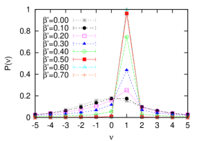
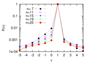
Figure 1: The probability distribution of the index $\nu$ is plotted for various $\beta^{\prime}$ at $n=15$ (left) and for various $n$ at $\beta^{\prime}=0.55$ (right). In the latter plot, the probability is plotted in the log scale to make the distribution at $\nu\neq 1$ visible.

8 Summary and discussions

In this paper we have constructed a finite-matrix formulation of gauge theories on a NC torus in a purely algebraic way. The configuration space has been defined as the representation space of coordinate and shift operators, which is analogous to projective modules in the continuum NC space. In particular, we are able to describe twisted boundary conditions and hence the Morita equivalence explicitly at a fully regularized level. Matter fields in the fundamental representation are represented by rectangular matrices analogously to the matrix spherical harmonics on the fuzzy sphere with the monopole background. By using the index of the overlap Dirac operator for the fundamental matter, we can classify the gauge field configurations into topological sectors. Monte Carlo results demonstrate that topologically nontrivial configurations survive the continuum limit of the NC gauge theory with twisted boundary conditions in a way consistent with the index theorem. This also confirms the validity of our formulation and its usefulness in various nonperturbative studies.

As we mentioned in the Introduction, one of our motivations for studying topological aspects of NC gauge theories is to understand the realization of a chiral gauge theory in our four-dimensional world by compactifying string theory with a nontrivial index in the extra dimensions. In this context, an interesting possibility would be that NC geometry is actually realized only in the extra dimensions as discussed in refs. [46] using the fuzzy sphere, where the dynamical generation of a nontrivial index may be possible [33]. Using our formulation, one can perform similar analyses using a NC torus. Considering the dramatic effects of NC geometry on topological properties [25], we may hope to obtain results qualitatively different from what we know for commutative extra dimensions.

Ultimately we hope to realize the whole set up dynamically, for instance, in the IIB matrix model [47], which is conjectured to be a nonperturbative definition of type IIB superstring theory in 10 dimensions. The dynamical generation of 4d space-time in this model is discussed, for instance in ref. [48, 49]. NC geometry appears naturally from the IIB matrix model for particular backgrounds [5], and this feature is recently focused also in the context of emergent gravity [50]. It would be interesting if one could describe the low energy effective theory of the IIB matrix model after dynamical generation of 4d space time in terms of field theory with NC extra dimensions.

Appendix A Some details of the review in Section 2

In this Appendix we present some details of the review given in section 2 to make it self-contained. We also refer the readers to ref. [36] for the topics that are not covered here.

A.1 NC gauge theory with twisted boundary conditions

In section 2 we described field theories on a NC geometry in terms of operators. In that language a field configuration $f(x)$ corresponds to the operator $\hat{f}$ through

$$\hat{f} = \int d^{D}x~{}\hat{\Delta}(x)f(x)\ ,$$ (99)

$$\hat{\Delta}(x) = \int\frac{d^{D}k}{(2\pi)^{D}}~{}{\,\rm e}\,^{ik_{\mu}\hat{x}_{\mu}}~{}e^{-ik_{\mu}x^{\mu}}\ ,$$ (100)

where the coordinate operators $\hat{x}_{\mu}$ and the derivative operators $\hat{\partial}_{\mu}$ satisfy the algebra (1). The product of two fields $f(x)$ and $g(x)$ are defined by the operator product of the corresponding operators $\hat{f}$ and $\hat{g}$, and it can be given explicitly by the so-called Moyal star-product

$$f(x)\star g(x)=f(x)~{}\exp\left(\frac{i}{2}\,\overleftarrow{\partial_{\mu}}\,\theta_{\mu\nu}\,\overrightarrow{\partial_{\nu}}\right)~{}g(x)\ ,$$ (101)

where $\theta_{\mu\nu}$ is the NC parameter appearing in (1).

Let us consider a U($p$) gauge theory on a NC torus, whose action is given by

$$S_{\rm YM} = \frac{1}{4g^{2}}\,\int_{{\bf T}^{D}}d^{D}x~{}{\rm tr\,}^{~{}}_{p}\Bigl{(}F_{\mu\nu}(x)-f_{\mu\nu}\,\Bigr{)}_{\star}^{2}\ ,$$ (102)

$$F_{\mu\nu}(x) = \partial_{\mu}A_{\nu}(x)-\partial_{\nu}A_{\mu}(x)-i\Bigl{(}A_{\mu}(x)\star A_{\nu}(x)-A_{\nu}(x)\star A_{\mu}(x)\Bigr{)}\ .$$ (103)

The constant background flux $f_{\mu\nu}$ will be specified later. We require the gauge field $A_{\mu}(x)$ to obey the twisted boundary conditions

$$A_{\mu}(x+L\hat{\nu})=\Omega_{\nu}(x)\star A_{\mu}(x)\star\Omega_{\nu}(x)^{\dagger}+i\,\Omega_{\nu}(x)\star\partial_{\mu}\,\Omega_{\nu}(x)^{\dagger}\ ,$$ (104)

where $\Omega_{\nu}(x)$ are the transition functions, which are $p\times p$ star-unitary matrices. The symbol $\hat{\nu}$ represents a unit vector in the $\nu$ direction. Consistency of the conditions (104) requires the transition functions $\Omega_{\mu}(x)$ to satisfy the co-cycle conditions

$$\Omega_{\mu}(x+L\hat{\nu})\star\Omega_{\nu}(x)=\Omega_{\nu}(x+L\hat{\mu})\star\Omega_{\mu}(x)\ .$$ (105)

It is convenient to introduce a background abelian gauge field $A^{(0)}_{\mu}(x)$, which obeys the twisted boundary conditions (104), and to decompose the gauge field configuration $A_{\mu}(x)$ into the background and the fluctuation as

$$A_{\mu}(x)=A^{(0)}_{\mu}(x)+{\cal A}_{\mu}(x)\ .$$ (106)

Then the boundary conditions for the fluctuation ${\cal A}_{\mu}(x)$ take the homogeneous form as

$${\cal A}_{\mu}(x+L\hat{\nu})=\Omega_{\nu}(x)\star{\cal A}_{\mu}(x)\star\Omega_{\nu}(x)^{\dagger}\ .$$ (107)

In order for $A^{(0)}_{\mu}(x)$ to give the minimum of the classical action (102), we choose the flux $f_{\mu\nu}$ in (102) to be

$$f_{\mu\nu}=\partial_{\mu}A^{(0)}_{\nu}(x)-\partial_{\nu}A^{(0)}_{\mu}(x)-i\left(A^{(0)}_{\mu}(x)\star A^{(0)}_{\nu}(x)-A^{(0)}_{\nu}(x)\star A^{(0)}_{\mu}(x)\right)\ .$$ (108)

Then the action (102) can be rewritten as

$$S_{\rm YM} = \frac{1}{4g^{2}}\,\int_{{\bf T}^{D}}d^{D}x~{}{\rm tr\,}^{~{}}_{p}\Bigl{(}{\cal F}_{\mu\nu}(x)\Bigr{)}_{\star}^{2}\ ,$$ (109)

$${\cal F}_{\mu\nu}(x) = D^{(0)}_{\mu}{\cal A}_{\nu}(x)-D^{(0)}_{\nu}{\cal A}_{\mu}(x)-i\Bigl{(}{\cal A}_{\mu}(x)\star{\cal A}_{\nu}(x)-{\cal A}_{\nu}(x)\star{\cal A}_{\mu}(x)\Bigr{)}\ ,$$ (110)

where we have defined the covariant derivative $D^{(0)}_{\mu}$ with the background field as

$$D^{(0)}_{\mu}=\partial_{\mu}-i\,[A^{(0)}_{\mu}(x)\,,~{}~{}~{}]_{\star}\ .$$ (111)

Using the map (99), we can define operators $\hat{A}_{\mu}$, $\hat{A}^{(0)}_{\mu}$, $\hat{\cal A}_{\mu}$ and $\hat{\Omega}_{\mu}$, which correspond to the fields $A_{\mu}(x)$, $A^{(0)}_{\mu}(x)$, ${\cal A}_{\mu}(x)$ and $\Omega_{\mu}(x)$, respectively. The action (109) can be written as

$$S_{\rm YM}=\frac{1}{4g^{2}}\,\mbox{Tr\,}\otimes{\rm tr\,}^{~{}}_{p}\left(\left[\hat{D}^{(0)}_{\mu}\,,\,\hat{\cal A}_{\nu}\right]-\left[\hat{D}^{(0)}_{\nu}\,,\,\hat{\cal A}_{\mu}\right]-i\left[\hat{\cal A}_{\mu}\,,\,\hat{\cal A}_{\nu}\right]\right)^{2}\ ,$$ (112)

where $\hat{D}^{(0)}_{\mu}$ is given by (5). The twisted boundary conditions (107) for ${\cal A}_{\mu}(x)$ can be written as (8). The background flux (108) is written as (6).

A.2 Explicit forms of the background gauge field and the transition functions

Let us consider the 2d case, and take the background gauge field as

$$\hat{A}^{(0)}_{1}=0\ ,\ \ \hat{A}^{(0)}_{2}=\hat{x}_{1}F\otimes{1\!\!1}_{p}\ .$$ (113)

Then the covariant derivative operators are given as

$$\hat{D}_{1}^{(0)}=\hat{\partial}_{1}\otimes{1\!\!1}_{p}\ ,\ \ \hat{D}_{2}^{(0)}=(\hat{\partial}_{2}-i\hat{x}_{1}F)\otimes{1\!\!1}_{p}\ ,$$ (114)

and the background abelian flux is obtained as $f_{12}=F$ by using (6).

We also assume that the transition function takes the form (9), where $\alpha_{\mu\nu}$ should be determined by requiring the background field (113) to obey the twisted boundary conditions

$${\,\rm e}\,^{L\hat{\partial}_{\nu}}~{}\hat{A}^{(0)}_{\mu}~{}{\,\rm e}\,^{-L\hat{\partial}_{\nu}}=\hat{\Omega}_{\nu}~{}\hat{A}^{(0)}_{\mu}~{}\hat{\Omega}_{\nu}^{\dagger}+i\,\hat{\Omega}_{\nu}\,[\hat{\partial}_{\mu},\hat{\Omega}_{\nu}^{\dagger}]\ .$$ (115)

Then the transition functions become

$$\hat{\Omega}_{1}={\,\rm e}\,^{i\frac{LF}{1+\theta F}\hat{x}_{2}}\otimes\Gamma_{1}^{(p)}\ ,\ \ \hat{\Omega}_{2}={1\!\!1}\otimes\Gamma_{2}^{(p)}\ ,$$ (116)

where $\theta_{\mu\nu}=\theta\varepsilon_{\mu\nu}$. Imposing the co-cycle conditions (105) on them, one can easily obtain (12). The covariantized transition functions $\hat{\Xi}$ defined by (28) can be expressed as

$$\hat{\Xi}_{1} = e^{i\frac{1}{1+\theta F}\hat{x}_{2}FL}\otimes\Gamma^{(p)}_{1}\ ,$$

$$\hat{\Xi}_{2} = e^{-i\hat{x}_{1}FL}\otimes\Gamma^{(p)}_{2}\ .$$ (117)

An explicit representation for $\Gamma_{\mu}^{(p)}$, which satisfy the ’t Hooft-Weyl algebra (10), can be given as

$$\Gamma^{(p)}_{1} = V_{\tilde{p}}\otimes{1\!\!1}_{p_{0}}\ ,$$

$$\Gamma^{(p)}_{2} = \left(W_{\tilde{p}}\right)^{-\tilde{q}}\otimes{1\!\!1}_{p_{0}}\ ,$$ (118)

where $V_{\tilde{p}}$ and $W_{\tilde{p}}$ are the SU($\tilde{p}$) shift and clock matrices

$$V_{\tilde{p}}=\begin{pmatrix}0&1&&&0\cr&0&1&&\cr&&\ddots&\ddots&\cr&&&\ddots&1\cr 1&&&&0\cr\end{pmatrix}\ ,\ \ W_{\tilde{p}}=\begin{pmatrix}1&&&&\cr&{\,\rm e}\,^{2\pi i/{\tilde{p}}}&&&\cr&&{\,\rm e}\,^{4\pi i/{\tilde{p}}}&&\cr&&&\ddots&\cr&&&&{\,\rm e}\,^{2\pi i({\tilde{p}}-1)/{\tilde{p}}}\cr\end{pmatrix}$$ (119)

obeying the commutation relations

$$V_{\tilde{p}}W_{\tilde{p}}={\,\rm e}\,^{2\pi i/{\tilde{p}}}\,W_{\tilde{p}}V_{\tilde{p}}\ .$$ (120)

A.3 Morita equivalence

We are now ready to solve the twisted boundary conditions (8). For any pair of co-prime integers $\tilde{p},\tilde{q}$, the set $\{(V_{\tilde{p}})^{j}\,(W_{\tilde{p}})^{\tilde{q}j^{\prime}}~{}|~{}j,j^{\prime}\in\mathbb{Z}_{\tilde{p}}\}$ spans the $\tilde{p}^{2}$ dimensional complex linear vector space. We therefore expand $\hat{\cal A}_{\mu}$ as

$$\hat{\cal A}_{\mu}=\int d^{2}k~{}{\,\rm e}\,^{ik_{\nu}\hat{x}_{\nu}}\otimes\sum_{\vec{j}~{}{\rm mod}\,\tilde{p}}~{}\prod_{\lambda=1}^{2}(\Gamma^{(\tilde{p})}_{\lambda})^{j_{\lambda}}\otimes\tilde{a}_{\mu}(\vec{k},\vec{j}\,)\ ,$$ (121)

where $\tilde{a}_{\mu}(\vec{k},\vec{j}\,)$ is a $p_{0}\times p_{0}$ matrix-valued function which has a periodicity $\tilde{p}$ in $\vec{j}$. By applying the conditions (8) to (121), and using (116), we find that the functions $\tilde{a}_{\mu}(\vec{k},\vec{j}\,)$ should vanish unless

$$\frac{1}{2\pi}\frac{1}{\tilde{p}}\left(\beta^{-1}\right)_{\mu\nu}k_{\nu}+\frac{\tilde{q}}{\tilde{p}}\varepsilon_{\mu\nu}j_{\nu}=n_{\mu}$$ (122)

for some $n_{\mu}\in\mathbb{Z}$, where $\beta_{\mu\nu}$ are defined as

$$\beta_{11}=\frac{1+\theta F}{L\tilde{p}}\ ,\ \ \beta_{22}=\frac{1}{L\tilde{p}}\ ,$$ (123)

and $\beta_{\mu\nu}=0$ for $\mu\neq\nu$. Using the integers $a,b$ introduced in (15), we can solve (122) by setting $n_{\mu}=a\,m_{\mu}$ and $j_{\mu}=b\,\varepsilon_{\mu\nu}\,m_{\nu}$ for some $m_{\mu}\in\mathbb{Z}$. Thus we obtain the momenta as $k_{\mu}=2\pi\beta_{\mu\nu}\,m_{\nu}$ and replace the integration in (121) by a sum over all $\vec{m}\in\mathbb{Z}^{2}$.

Therefore, the general solution to the conditions (8) takes the form (13), where $a_{\mu}(\vec{m})=\tilde{a}_{\mu}(2\pi\beta_{\mu\nu}m_{\nu},b\varepsilon_{\mu\nu}m_{\nu})$ are $p_{0}\times p_{0}$ matrix-valued Fourier coefficients. The operators $\hat{Z}^{\prime}_{\mu}$ are defined by (16), and more explicitly, they are given as

$$\hat{Z}^{\prime}_{1} = e^{2\pi i\frac{1+\theta F}{L\tilde{p}}\hat{x}_{1}}\otimes(\Gamma_{2}^{(p)})^{-b}\ ,$$

$$\hat{Z}^{\prime}_{2} = e^{2\pi i\frac{1}{L\tilde{p}}\hat{x}_{2}}\otimes(\Gamma_{1}^{(p)})^{b}\ .$$ (124)

They are shown to satisfy the algebra (17) and (18), and thus they are interpreted as the coordinate operators of the dual torus. While the derivation has been given in the specific gauge (113), the results (17) and (18) are gauge covariant, and the relations (20) and (21) are gauge invariant.

One can map the operators to periodic fields on the dual torus by

$${\cal A}^{\prime}_{\mu}(x^{\prime}) = \mbox{Tr\,}^{\prime}\left(\hat{\Delta}^{\prime}(x^{\prime})\hat{\cal A}_{\mu}\right)$$ (125)

$$\hat{\Delta}^{\prime}(x^{\prime}) = \frac{1}{L^{\prime 2}}\sum_{\vec{m}\in\mathbb{Z}^{2}}\,\prod_{\nu=1}^{2}\left(\hat{Z}^{\prime}_{\nu}\right)^{m_{\nu}}\,\prod_{\lambda<\rho}{\,\rm e}\,^{-\pi i\,m_{\lambda}\,\Theta^{\prime}_{\lambda\rho}\,m_{\rho}}{\,\rm e}\,^{-2\pi i\frac{1}{L^{\prime}}m_{\mu}x^{\prime}_{\mu}}\ ,$$ (126)

since $\hat{\cal A}_{\mu}$ can be expanded in terms of $\hat{Z}^{\prime}_{\mu}$ as in (13).

In terms of the fields (125), the action (112) can be written in arbitrary dimension $D$ as

$$S_{\rm YM} = \frac{1}{4g^{\prime 2}}\,\int d^{D}x^{\prime}~{}{\rm tr\,}^{~{}}_{p_{0}}\Bigl{(}{\cal F}_{\mu\nu}^{\prime}(x^{\prime})\Bigr{)}^{2}_{\star^{\prime}}\ ,$$ (127)

$${\cal F}_{\mu\nu}^{\prime}(x^{\prime}) = \partial_{\mu}^{\prime}{\cal A}_{\nu}^{\prime}(x^{\prime})-\partial_{\nu}^{\prime}{\cal A}_{\mu}^{\prime}(x^{\prime})-i\Bigl{(}{\cal A}_{\mu}^{\prime}(x^{\prime})\star^{\prime}{\cal A}_{\nu}^{\prime}(x^{\prime})-{\cal A}_{\nu}^{\prime}(x^{\prime})\star^{\prime}{\cal A}_{\mu}^{\prime}(x^{\prime})\Bigr{)}\ ,$$ (128)

where $\star^{\prime}$ denotes the new star-product with the NC parameter $\theta^{\prime}_{\mu\nu}=\frac{L^{\prime 2}}{2\pi}\Theta^{\prime}_{\mu\nu}$ instead of $\theta_{\mu\nu}$, and $\partial_{\mu}^{\prime}$ is the ordinary derivative operator on the dual NC torus. Since the operator trace $\mbox{Tr\,}^{\prime}$ is related to the original trace $\rm{Tr}$ by

$$\mbox{Tr\,}^{\prime}\otimes{\rm tr\,}^{~{}}_{p_{0}}=\frac{p_{0}}{p}\,\left|\frac{L^{\prime}}{L}\right|^{D}\,\mbox{Tr\,}\otimes{\rm tr\,}^{~{}}_{p}\ ,$$ (129)

the dual gauge coupling constant in (127) is related to the original one in (109) as

$$g^{\prime 2}=g^{2}\,\frac{p_{0}}{p}\,\left|\frac{L^{\prime}}{L}\right|^{D}\ .$$ (130)

References

- [1] H.S. Snyder, Quantized space-time, Phys. Rev. 71 (1947) 38.
- [2] A. Connes, Noncommutative geometry, Academic Press, 1990.
- [3] S. Doplicher, K. Fredenhagen and J.E. Roberts, The quantum structure of spacetime at the Planck scale and quantum fields, Commun. Math. Phys. 172 (1995) 187 [hep-th/0303037].
- [4] A. Connes, M. R. Douglas and A. Schwarz, Noncommutative geometry and matrix theory: Compactification on tori, J. High Energy Phys. 02 (1998) 003 [hep-th/9711162].
- [5] H. Aoki, N. Ishibashi, S. Iso, H. Kawai, Y. Kitazawa and T. Tada, Noncommutative Yang-Mills in IIB matrix model, Nucl. Phys. B 565 (2000) 176 [hep-th/9908141].
- [6] N. Seiberg and E. Witten, String theory and non-commutative geometry, J. High Energy Phys. 09 (1999) 032 [hep-th/9908142].
- [7] S. Minwalla, M. van Raamsdonk and N. Seiberg, Noncommutative perturbative dynamics, J. High Energy Phys. 02 (2000) 020 [hep-th/9912072].
- [8] I. Chepelev and R. Roiban, Renormalization of quantum field theories on noncommutative . I: Scalars, J. High Energy Phys. 0005 (2000) 037 [hep-th/9911098].
- [9] T. Eguchi and H. Kawai, Reduction of dynamical degrees of freedom in the large N gauge theory, Phys. Rev. Lett. 48 (1982) 1063.
- [10] A. González-Arroyo and M. Okawa, A twisted model for large lattice gauge theory, Phys. Lett. B 120 (1983) 174; The twisted Eguchi-Kawai model: a reduced model for large N lattice gauge theory, Phys. Rev. D 27 (1983) 2397.
- [11] J. Ambjørn, Y.M. Makeenko, J. Nishimura and R.J. Szabo, Finite N matrix models of noncommutative gauge theory, J. High Energy Phys. 11 (1999) 029 [hep-th/9911041]; Nonperturbative dynamics of noncommutative gauge theory, Phys. Lett. B 480 (2000) 399 [hep-th/0002158]; Lattice gauge fields and discrete noncommutative Yang-Mills theory, J. High Energy Phys. 05 (2000) 023 [hep-th/0004147].
- [12] W. Bietenholz, F. Hofheinz and J. Nishimura, A non-perturbative study of gauge theory on a non-commutative plane, J. High Energy Phys. 09 (2002) 009 [hep-th/0203151].
- [13] S.S. Gubser and S.L. Sondhi, Phase structure of non-commutative scalar field theories, Nucl. Phys. B 605 (2001) 395 [hep-th/0006119].
- [14] M. van Raamsdonk, The meaning of infrared singularities in noncommutative gauge theories, J. High Energy Phys. 0111 (2001) 006 [hep-th/0110093].
- [15] A. Armoni and E. Lopez, UV/IR mixing via closed strings and tachyonic instabilities, Nucl. Phys. B 632 (2002) 240 [hep-th/0110113].
- [16] J. Ambjørn and S. Catterall, Stripes from (noncommutative) stars, Phys. Lett. B 549 (2002) 253 [hep-lat/0209106].
- [17] W. Bietenholz, F. Hofheinz and J. Nishimura, Phase diagram and dispersion relation of the non-commutative model in , J. High Energy Phys. 0406 (2004) 042 [hep-th/0404020].
- [18] W. Bietenholz, J. Nishimura, Y. Susaki and J. Volkholz, A non-perturbative study of 4d U(1) non-commutative gauge theory: The fate of one-loop instability, J. High Energy Phys. 10 (2006) 042 [hep-th/0608072].
- [19] T. Azuma, S. Bal, K. Nagao and J. Nishimura, Nonperturbative studies of fuzzy spheres in a matrix model with the Chern-Simons term, J. High Energy Phys. 0405 (2004) 005 [hep-th/0401038].
- [20] T. Azeyanagi, M. Hanada and T. Hirata, On matrix model formulations of noncommutative Yang-Mills theories, arXiv:0806.3252.
- [21] R. Gopakumar, S. Minwalla and A. Strominger, Noncommutative solitons, J. High Energy Phys. 0005 (2000) 020 [hep-th/0003160]; J. A. Harvey, P. Kraus and F. Larsen, Exact noncommutative solitons, J. High Energy Phys. 0012 (2000) 024 [hep-th/0010060]. N. Nekrasov and A. Schwarz, Instantons on noncommutative and (2,0) superconformal six dimensional theory, Commun. Math. Phys. 198 (1998) 689 [hep-th/9802068]; A. P. Polychronakos, Flux tube solutions in noncommutative gauge theories, Phys. Lett. B 495 (2000) 407 [hep-th/0007043]; D. J. Gross and N. A. Nekrasov, Dynamics of strings in noncommutative gauge theory, J. High Energy Phys. 0010 (2000) 021 [hep-th/0007204]; M. Aganagic, R. Gopakumar, S. Minwalla and A. Strominger, Unstable solitons in noncommutative gauge theory, J. High Energy Phys. 0104 (2001) 001 [hep-th/0009142]; D. Bak, Exact multi-vortex solutions in noncommutative Abelian-Higgs theory, Phys. Lett. B 495 (2000) 251 [hep-th/0008204]; D. J. Gross and N. A. Nekrasov, Monopoles and strings in noncommutative gauge theory, J. High Energy Phys. 0007 (2000) 034 [hep-th/0005204];
- [22] H. Grosse, C. Klimcik and P. Presnajder, Topologically nontrivial field configurations in noncommutative geometry, Commun. Math. Phys. 178 (1996) 507 [hep-th/9510083]; S. Baez, A. P. Balachandran, B. Ydri and S. Vaidya, Monopoles and solitons in fuzzy physics, Commun. Math. Phys. 208 (2000) 787 [hep-th/9811169]; G. Landi, Projective modules of finite type and monopoles over S(2), J. Geom. Phys. 37 (2001) 47 [math-ph/9905014]; A. P. Balachandran and S. Vaidya, Instantons and chiral anomaly in fuzzy physics, Int. J. Mod. Phys. A 16 (2001) 17 [hep-th/9910129]; P. Valtancoli, Projectors for the fuzzy sphere, Mod. Phys. Lett. A 16 (2001) 639 [hep-th/0101189]; H. Steinacker, Quantized gauge theory on the fuzzy sphere as random matrix model, Nucl. Phys. B 679 (2004) 66 [hep-th/0307075]; D. Karabali, V. P. Nair and A. P. Polychronakos, Spectrum of Schroedinger field in a noncommutative magnetic monopole, Nucl. Phys. B 627 (2002) 565 [hep-th/0111249]; U. Carow-Watamura, H. Steinacker and S. Watamura, Monopole bundles over fuzzy complex projective spaces, J. Geom. Phys. 54 (2005) 373 [hep-th/0404130].
- [23] A. P. Balachandran and G. Immirzi, The fuzzy Ginsparg-Wilson algebra: A solution of the fermion doubling problem, Phys. Rev. D 68 (2003) 065023 [hep-th/0301242].
- [24] H. Aoki, J. Nishimura and Y. Susaki, The index of the overlap Dirac operator on a discretized 2d non-commutative torus, J. High Energy Phys. 0702 (2007) 033 [hep-th/0602078].
- [25] H. Aoki, J. Nishimura and Y. Susaki, Probability distribuion of the index in gauge theory on 2d non-commutative geometry, JHEP 0710, 024 (2007) [hep-th/0604093].
- [26] W. Frisch, H. Markum and H. Grosse, Instantons in two-dimensional noncommutative U(1) gauge theory, PoS LAT2007 (2007) 317.
- [27] H. Aoki, Y. Hirayama and S. Iso, Index theorem in spontaneously symmetry-broken gauge theories on fuzzy 2-sphere, Phys. Rev. D 78 (2008) 025028 [arXiv:0804.0568].
- [28] C. R. Gattringer, I. Hip and C. B. Lang, Quantum fluctuations versus topology: A study in U(1)2 lattice gauge theory, Phys. Lett. B 409 (1997) 371 [hep-lat/9706010].
- [29] G. ’t Hooft, A property of electric and magnetic flux in nonabelian gauge theories, Nucl. Phys. B 153 (1979) 141.
- [30] L. Griguolo and D. Seminara, Classical solutions of the TEK model and noncommutative instantons in two dimensions, J. High Energy Phys. 0403 (2004) 068 [hep-th/0311041].
- [31] H. Aoki, S. Iso and T. Maeda, Ginsparg-Wilson Dirac operator in the monopole backgrounds on the fuzzy 2-sphere, Phys. Rev. D 75 (2007) 085021 [hep-th/0610125].
- [32] G. Ishiki, S. Shimasaki, Y. Takayama and A. Tsuchiya, Embedding of theories with SU symmetry into the plane wave matrix model, J. High Energy Phys. 0611 (2006) 089 [hep-th/0610038]; T. Ishii, G. Ishiki, S. Shimasaki and A. Tsuchiya, Fiber Bundles and Matrix Models, Phys. Rev. D 77 (2008) 126015 [arXiv:0802.2782].
- [33] H. Aoki, S. Iso, T. Maeda and K. Nagao, Dynamical generation of a nontrivial index on the fuzzy 2-sphere, Phys. Rev. D 71 (2005) 045017 [hep-th/0412052], Erratum : Phys. Rev. D 71 (2005) 069905.
- [34] H. Aoki, S. Iso and K. Nagao, Ginsparg-Wilson relation and ’t Hooft-Polyakov monopole on fuzzy 2-sphere, Nucl. Phys. B 684 (2004) 162 [hep-th/0312199].
- [35] T. Ishii, G. Ishiki, S. Shimasaki and A. Tsuchiya, super Yang-Mills from the plane wave matrix model, arXiv:0807.2352; G. Ishiki, S. W. Kim, J. Nishimura and A. Tsuchiya, Deconfinement phase transition in super Yang-Mills theory on from supersymmetric matrix quantum mechanics, arXiv:0810.2884.
- [36] R. J. Szabo, Quantum field theory on noncommutative spaces, Phys. Rept. 378 (2003) 207 [hep-th/0109162].
-
[37]
P. van Baal and B. van Geemen,
A simple construction of twist eating solutions,
J. Math. Phys. 27 (1986) 455;
D.R. Lebedev and M.I. Polikarpov, Extrema of the twisted Eguchi-Kawai action and the finite Heisenberg group, Nucl. Phys. B 269 (1986) 285. - [38] S. R. Das, Quark fields in twisted reduced large N QCD, Phys. Lett. B 132 (1983) 155.
- [39] H. Neuberger, Exactly massless quarks on the lattice, Phys. Lett. B 417 (1998) 141 [hep-lat/9707022]; Vector like gauge theories with almost massless fermions on the lattice, Phys. Rev. D 57 (1998) 5417 [hep-lat/9710089]; More about exactly massless quarks on the lattice, Phys. Lett. B 427 (1998) 353 [hep-lat/9801031].
- [40] J. Nishimura and M. A. Vazquez-Mozo, Noncommutative chiral gauge theories on the lattice with manifest star-gauge invariance, J. High Energy Phys. 0108 (2001) 033 [hep-th/0107110].
- [41] S. Iso and K. Nagao, Chiral anomaly and Ginsparg-Wilson relation on the noncommutative torus, Prog. Theor. Phys. 109 (2003) 1017 [hep-th/0212284].
- [42] H. Aoki, S. Iso and K. Nagao, Ginsparg-Wilson relation, topological invariants and finite noncommutative geometry, Phys. Rev. D 67 (2003) 085005 [hep-th/0209223].
- [43] P. H. Ginsparg and K. G. Wilson, A remnant of chiral symmetry on the lattice, Phys. Rev. D 25 (1982) 2649.
- [44] M. Lüscher, Exact chiral symmetry on the lattice and the Ginsparg-Wilson relation, Phys. Lett. B 428 (1998) 342 [hep-lat/9802011].
- [45] P. Hasenfratz, V. Laliena and F. Niedermayer, The index theorem in QCD with a finite cut-off, Phys. Lett. B 427 (1998) 125 [hep-lat/9801021].
- [46] P. Aschieri, J. Madore, P. Manousselis and G. Zoupanos, Dimensional reduction over fuzzy coset spaces, J. High Energy Phys. 0404 (2004) 034 [hep-th/0310072]; P. Aschieri, T. Grammatikopoulos, H. Steinacker and G. Zoupanos, Dynamical generation of fuzzy extra dimensions, dimensional reduction and symmetry breaking, J. High Energy Phys. 0609 (2006) 026 [hep-th/0606021]; H. Steinacker and G. Zoupanos, Fermions on spontaneously generated spherical extra dimensions, arXiv:0706.0398.
- [47] N. Ishibashi, H. Kawai, Y. Kitazawa and A. Tsuchiya, A large-N reduced model as superstring, Nucl. Phys. B 498 (1997) 467 [hep-th/9612115].
- [48] H. Aoki, S. Iso, H. Kawai, Y. Kitazawa and T. Tada, Space-time structures from IIB matrix model, Prog. Theor. Phys. 99 (1998) 713 [hep-th/9802085].
- [49] J. Nishimura and F. Sugino, Dynamical generation of four-dimensional space-time in the IIB matrix model, J. High Energy Phys. 0205 (2002) 001 [hep-th/0111102].
- [50] H. Steinacker, Emergent gravity from noncommutative gauge theory, J. High Energy Phys. 0712 (2007) 049 [arXiv:0708.2426]; R. Delgadillo-Blando, D. O’Connor and B. Ydri, Geometry in transition: a model of emergent geometry, Phys. Rev. Lett. 100 (2008) 201601 [arXiv:0712.3011]; H. Grosse, H. Steinacker and M. Wohlgenannt, Emergent gravity, matrix models and UV/IR mixing, J. High Energy Phys. 0804 (2008) 023 [arXiv:0802.0973]; R. Delgadillo-Blando, D. O’Connor and B. Ydri, Matrix models, gauge theory and emergent geometry, arXiv:0806.0558; H. Steinacker, Emergent gravity and noncommutative branes from Yang-Mills matrix models, arXiv:0806.2032; H. S. Yang, Emergent spacetime and the origin of gravity, arXiv:0809.4728.