Fluctuations of current-driven domain walls in the non-adiabatic regime.

Abstract

We outline a general framework to determine the effect of non-equilibrium fluctuations on driven collective coordinates, and apply it to a current-driven domain wall in a nanocontact. In this case the collective coordinates are the domain-wall position and its chirality, that give rise to momentum transfer and spin transfer, respectively. We determine the current-induced fluctuations corresponding to these processes and show that at small frequencies they can be incorporated by two separate effective temperatures. As an application, the average time to depin the domain wall is calculated and found to be lowered by current-induced fluctuations. It is shown that current-induced fluctuations play an important role for narrow domain walls, especially at low temperatures.

I Introduction

Fluctuations play an important role in many areas of physics. The classic example is Brownian motion einstein1905 , for example of a colloidal particle in a suspension. The effect of collisions of the small particles, that constitute the suspension, with the colloid is modelled by stochastic forces. The strength of these forces is inferred from the famous fluctuation-dissipation theorem, which states that their variance is proportional to damping due to viscosity, and to temperature, and that their average is zero. If the suspension is driven out of equilibrium, the average force on the colloid will no longer be zero. Because of the non-equilibrium situation, the fluctuation-dissipation theorem in principle no longer holds, and the fluctuations cannot be determined from it anymore. Another explicit example of fluctuations in a driven system that do not obey the fluctuation-dissipation theorem is shot noise in the current in mesoscopic conductors, where the fluctuations are determined by the applied voltage instead of temperature. It is ultimately caused by the fact that the electric current is carried by discrete charge quanta, the electrons.beenakker1997

The non-equilibrium system on which we focus in this paper is a current-driven domain wall berger1984 ; berger1985 in a ferromagnetic conductor. Here the domain wall and the electrons play the role of the colloid and the suspension from the above example. There are two distinct processes that lead to current-induced domain-wall motion: spin transfer slonczewski1996 ; berger1996 and momentum transfer.tatara2004 Physically, momentum transfer corresponds to the force exerted on the domain wall by electrons that are reflected by the domain wall or transmitted with different momentum. Spin transfer corresponds to electrons whose spin follows the magnetization of the domain wall adiabatically, thereby exerting a torque on the domain wall. Most experiments grollier2003 ; klaui2003 ; yamaguchi2004 ; beach2005 ; yamanouchi2006 are in the adiabatic regime, where the electron spin follows the direction of magnetization adiabatically and where the spin-transfer torque is the dominant effect. The effect of spin relaxation on spin transfer in the adiabatic limit, leading to a dissipative spin-transfer torque, was discussed theoretically zhang2004 and experimentally.hayashi2007 ; heyne2008 The experiments by Feigenson et al. feigenson2007 with SrRuO₃ films, on the other hand, are believed to be in the non-adiabatic limit where domain walls are narrow compared to the Fermi wave length and momentum transfer is dominant. In this paper, we will mostly consider narrow domain walls in nanocontacts.bruno1999 ; versluijs2001 ; garcia1999

Apart from the forces and torques on the magnetization texture due to nonzero average current, there are also current-induced fluctuations on the magnetization foros2005 ; nunez2008 that ultimately have their origin in shot noise in the spin and charge current. Foros et al. foros2005 studied the effects of spin-current shot noise in single-domain ferromagnets, and found that for large voltage and low temperature the fluctuations are determined by the voltage and not by the temperature. Chudnovskiy et al. chudnovskiy2008 study spin-torque shot noise in magnetic tunnel junctions, and in Ref. [foros2008, ] Foros et al. consider a general magnetization texture and work out the current-induced magnetization noise and inhomogeneous damping in the adiabatic limit.

In this paper, we determine the effect of current-induced fluctuations on a domain wall in the non-adiabatic limit. We show that it leads to anisotropic damping and fluctuations and show that the fluctuations can be described by two separate voltage-dependent effective temperatures corresponding to momentum transfer and spin transfer. We show that these effective temperatures differ considerably from the actual temperature for parameter values used in experiments with nanocontacts. From our model, we also determine the momentum transfer and the adiabatic spin-transfer torque on the driven domain wall, as well as the damping corresponding to these processes.

II Model

In this section, we present a model for treating a domain wall out of equilibrium. We first develop a variational principle within the Keldysh formalism, and then work out the various Green’s functions within Landauer-Büttiker transport.

II.1 Keldysh Theory

We consider a one-dimensional model of spins coupled to conduction electrons. The action is on the Keldysh contour $C$ given by

$$S[\mathbf{\Omega}, \psi,\psi^{*}]=\int_{C}dt\bigg{\{}-E_{\rm MM}[\mathbf{\Omega}]$$

$$+\int\frac{dx}{a}\bigg{[}-\hbar\mathbf{A}(\mathbf{\Omega}(x,t))\cdot\frac{\partial\mathbf{\Omega}(x,t)}{\partial t}$$

$$+\frac{\Delta}{2}\sum_{\sigma,\sigma^{\prime}}\psi^{*}_{\sigma}(x,t)\mathbf{\Omega}(x,t)\cdot\boldsymbol{\tau}_{\sigma,\sigma^{\prime}}\psi_{\sigma^{\prime}}(x,t)$$

$$+\sum_{\sigma}\psi^{*}_{\sigma}(x,t)\left(i\hbar\frac{\partial}{\partial t}+\frac{\hbar^{2}\nabla^{2}}{2m}-V(x)\right)\psi_{\sigma}(x,t)\bigg{]}\bigg{\}}\;,\;$$ (1)

where $a$ is the lattice spacing, $\mathbf{A}(\mathbf{\Omega})$ is the fictitious vector potential that obeys $\boldsymbol{\nabla}_{\mathbf{\Omega}}\times\mathbf{A(\mathbf{\Omega})}=\mathbf{\Omega}$ and ensures precessional motion of $\mathbf{\Omega}$, $\Delta$ is the exchange-splitting energy, $\mathbf{\Omega}(x,t)$ a unit vector in the direction of the magnetization, $\boldsymbol{\tau}$ the vector of Pauli matrices, and $V(x)$ an arbitrary scalar potential. The fields $\psi^{*}_{\sigma},\psi_{\sigma}$ represent the conduction electrons with spin projection $\sigma\in\{\uparrow,\downarrow\}$. The micromagnetic energy functional $E_{\rm MM}[\mathbf{\Omega}]$ is given by

$$E_{\rm MM}[\mathbf{\Omega}]=-\int\frac{dx}{a} \Big{[}J\mathbf{\Omega}(x,t)\cdot\vec{\nabla}^{2}\mathbf{\Omega}(x,t)$$

$$-K_{\perp}\Omega_{y}^{2}(x,t)+K_{z}\Omega_{z}^{2}(x,t)\Big{]}\;,$$ (2)

with $J>0$ the spin stiffness and $K_{\perp}>0$ and $K_{z}>0$ the hard- and easy-axis anisotropy constants, respectively. The micromagnetic energy functional in Eq. (II.1) has stationary domain-wall solutions $\mathbf{\Omega}(x)=(\sin\theta_{\rm dw}\cos\phi_{\rm dw},\sin\theta_{\rm dw}\sin\phi_{\rm dw},\cos\theta_{\rm dw})$.tatara2004 These stationary solutions are the basis for a time-dependent variational ansatz given by

$$\theta_{\rm dw}=2\arctan\left\{e^{[x-X(t)]/\lambda}\right\}\;;\qquad\phi_{\rm dw}=\phi(t)\;,$$ (3)

where $\lambda$ is the domain-wall width. In the above, we have taken the domain-wall position $X(t)$ to be time dependent. Furthermore, $\phi(t)$ is the angle of the magnetization at the center with the easy-plane, the so-called chirality. Using the above ansatz, the first two terms in the action in Eq. (II.1) simplify to

$$S_{0}[X,\phi]=\hbar N\int_{C}dt\left[\frac{\dot{X}}{\lambda}\phi-\frac{K_{\perp}}{2}\sin 2\phi\right]\;.$$ (4)

Here, $N=2\lambda/a$ is the number of spins in the domain wall. Note that in three dimensions, the number of spins increases by a factor $A/a^{2}$, where $A$ is the cross-sectional area of the sample.

Stochastic forces are not obtained in a natural way by variation of the real-time action or the Euclidean action of the system. The functional Keldysh formalism,footnotestoof however, provides us with the (current-induced and thermal) noise terms automatically, and is therefore more elegant for our purposes. By doing perturbation theory in the collective coordinates $X$ and $\phi$

$$\mathbf{\Omega}=\mathbf{\Omega}\Big{|}_{0}+X\frac{\partial\mathbf{\Omega}}{\partial X}\Big{|}_{0}+\phi\frac{\partial\mathbf{\Omega}}{\partial\phi}\Big{|}_{0}+{\rm h.o.}\;,$$ (5)

where from here onward the subscript $|_{{}_{0}}$ denotes evaluation at $X=\phi=0$, we derive an effective action on the Keldysh contour for the collective coordinates. We consider the low-frequency limit, which is a good approximation because the motion of the collective coordinates is on a much slower time scale than the electronic system.

The total action is now given by $S[X,\phi,\psi^{*},\psi]=S_{0}[X,\phi]+S_{\rm C}[X,\phi,\psi^{*},\psi]+S_{\rm E}[\psi^{*},\psi]$. The contribution to the action in Eq. (II.1) that describes coupling between magnetization and electrons is up to first order given by

$$S_{\rm C} [X,\phi]\Big{|}_{0}=\frac{\Delta}{2}\int_{C}dt\int dx\sum_{\sigma,\sigma^{\prime}}\psi^{*}_{\sigma}(x,t)$$

$$\Big{[}(\partial_{X}\boldsymbol{\Omega}\cdot\boldsymbol{\tau})\Big{|}_{0}X(t)+(\partial_{\phi}\boldsymbol{\Omega}\cdot\boldsymbol{\tau})\Big{|}_{0}\phi(t)\Big{]}\psi_{\sigma^{\prime}}(x,t),$$ (6)

where $\sigma$ and $\sigma^{\prime}$ denote the spin of the electrons. The electron action reads

$$S_{\rm E}[\psi^{*},\psi]=\int_{C}dt\int dx\sum_{\sigma,\sigma^{\prime}}\;\psi^{*}_{\sigma}(x,t)$$

$$\left[\left(i\hbar\frac{\partial}{\partial t}+\frac{\hbar^{2}\nabla^{2}}{2m}-V(x)\right)\delta_{\sigma\sigma^{\prime}}-V_{\sigma\sigma^{\prime}}(x)\right]\psi_{\sigma^{\prime}}(x,t)\;,$$ (7)

with the potential $V_{\sigma\sigma^{\prime}}$, which arises from the zeroth order term $\mathbf{\Omega}|_{0}$, given in Eq. (24) below. The perturbation theory in $X$ and $\phi$ enables us to derive an effective action on the Keldysh contour for these coordinates

$$S_{\rm eff} [X,\phi]\simeq S_{0}[X,\phi]+\langle S_{\rm C}[X,\phi,\psi^{*},\psi]\rangle$$

$$+ \frac{i}{2\hbar}\Big{(}\langle S_{\rm C}^{2}[X,\phi,\psi^{*},\psi]\rangle-\langle S_{\rm C}[X,\phi,\psi^{*},\psi]\rangle^{2}\Big{)}\;.$$ (8)

Here, the expectation values are taken with respect to the electron action $S_{\rm E}[\psi^{*},\psi]$ in Eq. (II.1), i.e.,

$$\langle O[X,\phi, \psi^{*},\psi]\rangle=$$

$$\int d[\psi^{*}]d[\psi]e^{iS_{\rm E}[\psi^{*},\psi]/\hbar}O[X,\phi,\psi^{*},\psi]\;.$$ (9)

In the next section, we evaluate these expectation values in more detail.

Since we now have an effective action as a function of the collective coordinates $X$ and $\phi$, we can make use of the advantages of the Keldysh formalism. The effective action in Eq. (II.1) is integrated from $t=-\infty$ to $t=\infty$ and back.

Figure 1: A path that the coordinate $X$ might take on the Keldysh contour. The deviation from the (classical) mean path is denoted by $\xi(t)$.

The forward and backward paths are different, as is shown for the coordinate $X$ in Fig.1, such that we write

$$X(t^{\pm})=X_{\rm cl}(t)\pm\frac{\xi(t)}{2}\;;\qquad \phi(t^{\pm})=\phi_{\rm cl}(t)\pm\frac{\kappa(t)}{2}\;;$$

$$\int_{C}dtf(t)=\int_{-\infty}^{\infty}dt^{+}f(t^{+}) +\int_{\infty}^{-\infty}dt^{-}f(t^{-})\;,$$ (10)

with the assumption that the variations $\xi$ and $\kappa$ are small. Furthermore, they obey the boundary conditions $\xi(\pm\infty)=\kappa(\pm\infty)=0$. Integrating the effective action over this contour and using the method outlined in Refs. [footnotestoof, ; nunez2008, ], we ultimately obtain the Langevin equations for a domain wall

$$\frac{\dot{X}_{\rm cl}(t)}{\lambda}-\alpha_{\phi}\dot{\phi}_{\rm cl}(t)=K_{\perp}\cos 2\phi_{\rm cl}(t)+F_{\phi}+ \eta_{\phi}(t)\;,$$ (11)

$$\dot{\phi}_{\rm cl}(t)+\alpha_{X}\frac{\dot{X}_{\rm cl}(t)}{\lambda}=-F_{X}+\eta_{X}(t)\;.$$ (12)

The stochastic contributions $\eta_{\phi}$ and $\eta_{X}$ in this expression arise via a Hubbard-Stratonovich transformation of terms quadratic in $\xi$ and $\kappa$.

The expectation value of the action $S_{C}[X,\phi,\psi^{*},\psi]$ in the effective action in Eq. (II.1) provide us with the forces

$$F_{i}=\frac{\Delta}{\hbar N}\sum_{\nu,\sigma,\sigma^{\prime}}G^{<}_{\nu,\sigma,\sigma^{\prime}}(0)\langle\nu,\sigma|\partial_{i}\boldsymbol{\Omega}|_{0}\cdot\boldsymbol{\tau}|\nu,\sigma^{\prime}\rangle\;,$$ (13)

where the index $i\in\{X/\lambda,\phi\}$. Note that in this expression, $F_{\phi}$ corresponds to spin transfer and $F_{X}$ to momentum transfer. As we will see later on, $\partial_{\phi}\mathbf{\Omega}|_{0}\cdot\boldsymbol{\tau}$ is associated with the divergence of the spin current, and $\partial_{X}\mathbf{\Omega}|_{0}\cdot\boldsymbol{\tau}$ is associated with the force of the domain wall on the conduction electrons. The latter is, in the absence of disorder, proportional to the resistance of the domain wall.tatara2004 The lesser Green’s function in this expression is defined by $G_{\nu,\sigma,\sigma^{\prime}}(t,t^{\prime})=\theta(t,t^{\prime})G^{>}_{\nu,\sigma,\sigma^{\prime}}(t-t^{\prime})+\theta(t^{\prime},t)G^{<}_{\nu,\sigma,\sigma^{\prime}}(t-t^{\prime})$, where the Heaviside step functions are defined on the Keldysh contour. Note that the lesser Green’s function in Eq. (13) is evaluated at equal times $t=t^{\prime}$. Furthermore, we have expanded the Keldysh Green’s function according to ${\rm i}G_{\sigma,\sigma^{\prime}}(x,t;x^{\prime},t^{\prime})\equiv\langle\psi_{\sigma}(x,t)\psi^{*}_{\sigma^{\prime}}(x^{\prime},t^{\prime})\rangle={\rm i}\sum_{\nu}G_{\nu,\sigma,\sigma^{\prime}}(t,t^{\prime})\chi_{\nu,\sigma}(x)\chi_{\nu,\sigma^{\prime}}^{*}(x^{\prime})$, where $\chi$ and $\chi^{*}$ are electron eigenstates in the presence of a static domain wall that are labeled by $\nu$. In terms of these states, the matrix elements are defined as

$$\int dx\;\langle\nu,\sigma|\hat{O}|\nu^{\prime},\sigma^{\prime}\rangle=\int dx\chi_{\nu,\sigma}(x)\hat{O}_{\sigma,\sigma^{\prime}}(x)\chi_{\nu^{\prime},\sigma^{\prime}}^{*}(x)\;.$$ (14)

The damping terms in Eqs. (11) and (12) follow from the second-order terms in the perturbation theory in $X$ and $\phi$ and read $\alpha_{i}=\mp{\rm Im}[\tilde{\Pi}^{(\pm)}_{i}(\omega)]/(N\hbar\omega)$ for $\omega\rightarrow 0$, with $\tilde{\Pi}^{(\pm)}(\omega)$ the response function given below. Since the action in Eq. (II.1) is quadratic in the electron fields, we use Wick’s theorem to write the response function in terms of electron Green’s functions

$$\tilde{\Pi}^{(\pm)}_{i}(\omega)=\mp\frac{\Delta^{2}}{4\hbar}\sum_{\nu,\nu^{\prime}}\sum_{\sigma,\sigma^{\prime}}\sum_{\rho,\rho^{\prime}}$$

$$\times\Big{[}G^{>}_{\nu,\sigma,\rho^{\prime}}(\omega)G^{<}_{\nu^{\prime},\rho,\sigma^{\prime}}(-\omega)-G^{<}_{\nu,\sigma,\rho^{\prime}}(\omega)G^{>}_{\nu^{\prime},\rho,\sigma^{\prime}}(-\omega)\Big{]}$$

$$\times\langle\nu,\sigma|\partial_{i}\boldsymbol{\Omega}|_{0}\cdot\boldsymbol{\tau}|\nu^{\prime},\sigma^{\prime}\rangle\langle\nu^{\prime},\rho|\partial_{i}\boldsymbol{\Omega}|_{0}\cdot\boldsymbol{\tau}|\nu,\rho^{\prime}\rangle\;.$$ (15)

The functions $G^{>}(\pm\omega)$ and $G^{<}(\pm\omega)$ denote Fourier transforms of $G^{>}(\pm(t-t^{\prime}))$ and $G^{<}(\pm(t-t^{\prime}))$, respectively.

Without needing to assume (approximate) equilibrium, the Keldysh formalism provides us with an expression for the strength of the fluctuations in both coordinates $\langle\eta_{i}(t)\eta_{j}(t^{\prime})\rangle={\rm i}\delta_{i,j}\Pi^{\rm K}_{i}(t-t^{\prime})/(\hbar N^{2})\simeq{\rm i}\delta_{i,j}\tilde{\Pi}^{\rm K}_{i}(\omega=0)\delta(t-t^{\prime})/(\hbar N^{2})$ and $\langle\eta_{i}(t)\rangle=0$. The Keldysh component of the response function contains similar matrix elements as the damping terms and is given by

$$\tilde{\Pi}^{\rm K}_{i}(\omega)=\frac{\Delta^{2}}{2\hbar}\sum_{\nu,\nu^{\prime}}\sum_{\sigma,\sigma^{\prime}}\sum_{\rho,\rho^{\prime}}$$

$$\times\Big{[}G^{>}_{\nu,\sigma,\rho^{\prime}}(\omega)G^{<}_{\nu^{\prime},\rho,\sigma^{\prime}}(-\omega)+G^{<}_{\nu,\sigma,\rho^{\prime}}(\omega)G^{>}_{\nu^{\prime},\rho,\sigma^{\prime}}(-\omega)\Big{]}$$

$$\times\langle\nu,\sigma|\partial_{i}\boldsymbol{\Omega}|_{0}\cdot\boldsymbol{\tau}|\nu^{\prime},\sigma^{\prime}\rangle\langle\nu^{\prime},\rho|\partial_{i}\boldsymbol{\Omega}|_{0}\cdot\boldsymbol{\tau}|\nu,\rho^{\prime}\rangle\;.$$ (16)

We now define two separate effective temperatures

$${\rm k}_{\rm B}T_{{\rm eff},i}\equiv\frac{{\rm i}\tilde{\Pi}_{i}^{\rm K}(\omega=0)}{2\alpha_{i}N^{2}}\;.$$ (17)

These effective temperatures are defined such that Eqs. (11) and (12) obey the fluctuation-dissipation theorem with the effective temperatures. In the absence of a bias voltage, the effective temperatures reduce to the actual temperature divided by the number of spins in the system. More general, the effective temperatures are proportional to $1/N$, which is understood because they describe fluctuations in collective coordinates made up of $N$ degrees of freedom.duine2007 We note that our formalism applies to any set of collective coordinates, and is not necessarily restricted to the example of a domain wall. We also point out that going beyond the low-frequency limit and taking into account the full frequency dependence in Eq. (II.1) leads to colored noise. In this case, effective temperatures may no longer be unambiguously defined.mitra2005

II.2 Landauer-Büttiker transport

We now evaluate Eqs. (13–II.1) using the Landauer-Büttiker formalism, i.e., the scattering theory of electronic transport. In order for this formalism to apply, the phase-coherence length $L_{\phi}$ must be larger than the domain-wall width $\lambda$. To compute the terms in the Langevin equations (11) and (12) explicitly, we need to find the matrix elements $\langle\nu,\sigma|\partial_{i}\mathbf{\Omega}|_{0}\cdot\boldsymbol{\tau}|\nu^{\prime},\sigma^{\prime}\rangle$ and the Green’s functions. The Keldysh Green’s function is in terms of scattering states $\chi^{\zeta\kappa\varepsilon}_{\sigma}(x)$ given by

$${\rm i}G_{\sigma,\sigma^{\prime}}(x,t;x^{\prime},t^{\prime})\qquad\qquad\qquad$$

$$=\int_{0}^{\infty}\frac{d\varepsilon}{2\pi}\sum_{\zeta,\kappa}\frac{2m/\hbar^{2}}{k_{\zeta\kappa}}e^{-\frac{{\rm i}}{\hbar}\varepsilon(t-t^{\prime})}\chi^{\zeta\kappa\varepsilon}_{\sigma^{\prime}}(x)[\chi^{\zeta\kappa\varepsilon}_{\sigma}(x^{\prime})]^{*}$$

$$\times\{\theta(t,t^{\prime})[1-N_{\rm F}(\varepsilon-\mu_{\zeta})]-\theta(t^{\prime},t)N_{\rm F}(\varepsilon-\mu_{\zeta})\}\;,$$ (18)

with $\mu_{\zeta}$ the chemical potential of the lead on side $\zeta\in\{{\rm L(eft),R(ight)}\}$, $\kappa\in\{\uparrow,\downarrow\}$ the spin of the incoming particles and $N_{\rm F}(x)$ the Fermi distribution function. We choose $V(x)=0$ for convenience. The momenta $k_{\zeta\kappa}$ associated with an energy $\varepsilon$ are given by $k_{{\rm L}\uparrow}=k_{{\rm R}\downarrow}=k_{\rm F}\sqrt{(\varepsilon+\Delta/2)/\varepsilon_{\rm F}\;}$ and $k_{{\rm R}\uparrow}=k_{{\rm L}\downarrow}=k_{\rm F}\sqrt{(\varepsilon-\Delta/2)/\varepsilon_{\rm F}\;}$, where $k_{\rm F}=\sqrt{2m\varepsilon_{\rm F}/\hbar^{2}}$, with $\varepsilon_{\rm F}$ the Fermi energy in the leads. Note that the index $\nu$ used earlier now contains information on the origin, spin and energy of the incoming particle. We define the asymptotic expression for the scattering states in terms of transmission and reflection coefficients,

$$\chi_{\sigma}^{{\rm L}\kappa\varepsilon}\!=\!\left\{\begin{array}[]{cl}\!\!\delta_{\sigma,\kappa}e^{{\rm i}k_{{\rm L}\kappa}x}\!+\delta_{\sigma,\gamma}\sqrt{\frac{k_{{\rm L}\kappa}}{k_{{\rm L}\gamma}}}r_{\gamma\kappa}(\varepsilon)e^{-{\rm i}k_{{\rm L}\gamma}x},&x\rightarrow\!-\infty\;;\\ \\ \delta_{\sigma,\gamma}\sqrt{\frac{k_{{\rm L}\kappa}}{k_{{\rm R}\gamma}}}t_{\gamma\kappa}(\varepsilon)e^{{\rm i}k_{{\rm R}\gamma}x},&x\rightarrow\!+\infty\;,\end{array}\right.$$ (22)

where summation over spin-index $\gamma\in\{\uparrow,\downarrow\}$ is implied, and with a similar expression for right-incoming particles. From the explicit form of the ansatz, it is easily seen that $\partial\mathbf{\Omega}/\partial X=-\partial\mathbf{\Omega}/\partial x$ which enables us to write $(\Delta/2)(\partial\mathbf{\Omega}/\partial X)|_{0}\cdot\boldsymbol{\tau}_{\sigma,\sigma^{\prime}}=\partial_{x}V_{\sigma,\sigma^{\prime}}(x)$. Here $\partial_{x}$ denotes a derivative with respect to $x$, and the potential is given by

$$V_{\sigma\sigma^{\prime}}(x)=-\frac{\Delta}{2}\begin{pmatrix}\cos\theta_{\rm dw}&\sin\theta_{\rm dw}\\ \\ \sin\theta_{\rm dw}&-\cos\theta_{\rm dw}\end{pmatrix}\Bigg{|}_{0}\;.$$ (24)

Furthermore, one can check that $(\partial\mathbf{\Omega}/\partial\phi)\cdot\boldsymbol{\tau}_{\sigma\sigma^{\prime}}|_{0}=-(\boldsymbol{\tau}_{\sigma\sigma^{\prime}}\times\mathbf{\Omega})|^{z}_{0}$, where uppercase $z$ denotes the $z$ component of this cross product. The expectation value of this quantity is directly related to the divergence of the spin-current $J_{\rm s}^{z}$, which measures the $z$ component of the total spin-current

$$\partial_{x}J^{z}_{\rm s}(x)=\frac{\Delta}{2}\sum_{\sigma,\sigma^{\prime}}\chi^{*}_{\sigma}(x)\Big{[}\boldsymbol{\tau}_{\sigma\sigma^{\prime}}\times\mathbf{\Omega}(x)\Big{]}^{z}_{0}\chi_{\sigma^{\prime}}(x)\;.$$ (25)

In this expression, $\chi$ is a solution to the zeroth order time-independent Schrödinger equation with the potential $V_{\sigma,\sigma^{\prime}}(x)$. The spin current is defined as

$$J_{\rm s}^{z}(x)=\frac{\hbar^{2}}{4mi}\sum_{\sigma,\sigma^{\prime}}\Big{\{} \chi^{*}_{\sigma}(x)\tau_{\sigma\sigma^{\prime}}^{z}[\partial_{x}\chi_{\sigma^{\prime}}(x)]$$

$$\;\;-[\partial_{x}\chi^{*}_{\sigma}(x)]\tau_{\sigma\sigma^{\prime}}^{z}\chi_{\sigma^{\prime}}(x)\Big{\}}\;.$$ (26)

From this, we observe that $F_{\phi}$ determined by Eq. (13) is indeed proportional to the divergence of spin current and hence corresponds to spin transfer.

We define $\mu_{\rm L}=\mu+|e|V$ and $\mu_{\rm R}=\mu\simeq\varepsilon_{\rm F}$. The expressions for the Green’s function and the scattering states in Eqs. (II.2) and (22) now allow us to write Eqs. (13–17) in terms of transmission and reflection coefficients, the applied voltage $V$, and $k_{\rm F}\lambda$. For example, the momentum transfer in Eq. (13), with $i=X$, is up to first order in $|e|V/\varepsilon_{\rm F}$ given by

$$F_{X}\simeq\frac{|e|V}{2\pi\hbar N}k_{\rm F}\lambda$$

$$\Bigg{[}\sqrt{\frac{\varepsilon+\Delta/2}{\varepsilon_{\rm F}}}\Big{(}1+R_{\uparrow\uparrow}-T_{\downarrow\downarrow}+R_{\uparrow\downarrow}-T_{\downarrow\uparrow}\Big{)}$$

$$+\sqrt{\frac{\varepsilon-\Delta/2}{\varepsilon_{\rm F}}}\Big{(}1+R_{\downarrow\downarrow}-T_{\uparrow\uparrow}+R_{\downarrow\uparrow}-T_{\uparrow\downarrow}\Big{)}\Bigg{]}\;,$$ (27)

Here, the reflection and transmission coefficients are defined as $R_{\sigma\sigma^{\prime}}=R_{\sigma\sigma^{\prime}}(\varepsilon=\varepsilon_{\rm F})$ with $R_{\sigma\sigma^{\prime}}(\varepsilon)\equiv|r_{\sigma\sigma^{\prime}}(\varepsilon)|^{2}$, and equivalently for the transmission coefficients. Note that, although the coefficients are evaluated at the Fermi energy, they also depend on the ratio $\Delta/\varepsilon_{\rm F}$. The expression for the momentum transfer in Eq. (II.2) clearly demonstrates its correspondence to electrons scattering off the domain wall: it increases for increasing reflection and decreases for increasing transmission.

The explicit form of the spin-transfer torque $F_{\phi}$ has $\propto T_{\downarrow\uparrow}$ as leading term, which is a measure for the number of electrons that follow the domain-wall magnetization.

The reflection and transmission coefficients are obtained by solving the Schrödinger equation of the system numerically, and matching the results to the asymptotic behavior in Eq. (22). As an example, we present the coefficients for $\Delta/2\varepsilon_{\rm F}=0.8$ as a function of $k_{\rm F}\lambda$ in Fig. 2.

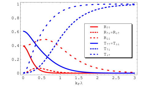
Figure 2: (color online). Transmission and reflection coefficients as functions of $k_{\rm F}\lambda$ for $\Delta/2\varepsilon_{\rm F}=0.8$ and $V=0$.

III Results

As we have shown in the previous section, we are able to express Eqs. (13–II.1) in terms of transmission and reflection coefficients using Landauer-Büttiker transport, like in Eq. (II.2). As indicated, these coefficients are obtained by numerically solving the Schrödinger equation.

In the limit of vanishing voltage, Eq. (II.2) is the exact expression for the momentum transfer. In fact, the momentum transfer as well as the spin-transfer torque are for small $|e|V/\varepsilon_{\rm F}$ proportional to the voltage, in agreement with the fact that these quantities are usually described as linear with the spin current.tatara2004 We present the ratio of these forces that measures the degree of nonadiabaticity, denoted by $F_{X}/F_{\phi}=\beta$, as a function of $k_{\rm F}\lambda$ for several values $\Delta/2\varepsilon_{\rm F}$ in Fig. 3.

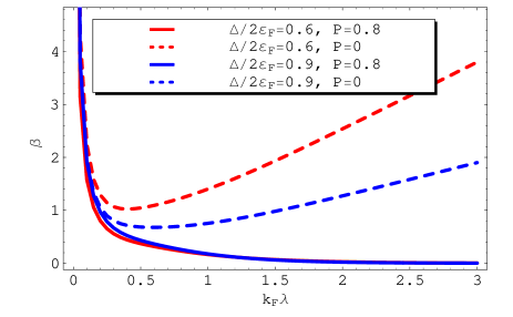
Figure 3: (color online). The parameter $\beta=F_{X}/F_{\phi}$ as a function of $k_{\rm F}\lambda$ for $\Delta/2\varepsilon_{\rm F}=0.6$ and $\Delta/2\varepsilon_{\rm F}=0.9$, both at zero voltage. The dashed curves are obtained by ignoring polarization, the solid lines are obtained for a polarization of $P=0.8$.

In Fig. 3, the dashed curves show the result obtained directly from Eq. (II.2) and an equivalent expression for $F_{\phi}$. We see that $\beta$ is large for small $k_{\rm F}\lambda$, as expected. The ratio, however, does not vanish for large $k_{\rm F}\lambda$, which one would expect, but instead acquires a linear dependence on $k_{\rm F}\lambda$. Mathematically, this is caused not by an increase of momentum transfer, but instead by a vanishing spin transfer. We can make sure that the spin transfer does not vanish by taking into account the polarization of the incoming electron current.mazin1999 ; waintal2004 . If we do take this into account, such that $R_{\sigma\uparrow}\rightarrow R_{\sigma\uparrow}(1+P)$, $R_{\sigma\downarrow}\rightarrow R_{\sigma\downarrow}(1-P)$, and equivalently for transmission coefficients, we find for $P=0.8$ the solid curves in Fig. 3. We see that these curves indeed go to zero in the adiabatic limit $k_{\rm F}\lambda\gg 1$. From Fig. 3, it is clear that the polarization plays a big role from values $k_{\rm F}\lambda\simeq 0.3$ onwards. Note that our theory does not take into account the dissipative spin-transfer torque, which gives similar contributions as momentum trensfer.zhang2004

For the damping parameters $\alpha_{X}$ and $\alpha_{\phi}$, we find that for small $|e|V/\varepsilon_{\rm F}$, they both acquire corrections linear in the voltage, in agreement with Katsura et al. katsura2006 and Núñez and Duine.nunez2008 The dependence on $k_{\rm F}\lambda$ is much less trivial, as is shown in Fig. 4, where the curves are taken at zero voltage.

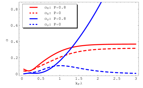
Figure 4: (color online). The damping parameters $\alpha_{X}$ and $\alpha_{\phi}$ as a function of $k_{\rm F}\lambda$ for $\Delta/2\varepsilon_{\rm F}=0.9$, both at zero voltage. The dashed curves are obtained by ignoring polarization, the solid lines are obtained for a polarization of $P=0.8$.

The unpredictable behavior of the damping parameters as a function of $k_{\rm F}\lambda$ for small $k_{\rm F}\lambda$ arises from the details of the solutions of the Schrödinger equation. For large $k_{\rm F}\lambda$, we see that without polarization $\alpha_{\phi}$ goes to zero, whereas for nonzero polarization, it increases quadratically. This is understood from the fact that damping in the angle $\phi$ arises from emission of spin waves. This in its turn is closely related to spin-transfer torque, which goes to zero for $P=0$ but assumes nonzero values for $P>0$, as was discussed earlier in this section. It should be noted, however, that this approach breaks down for large values $k_{\rm F}\lambda$ since we then lose phase coherence as $\lambda>L_{\phi}$. Furthermore, the polarization could be addressed in a more rigorous way by taking into account more transverse channels. Note that the fact that $\alpha_{X}\neq\alpha_{\phi}$ is a specific example of inhomogeneous damping as discussed by Foros et al..foros2008

The effective temperatures of the system depend on the dimensionless parameters $k_{\rm F}\lambda$ and $\Delta/2\varepsilon_{\rm F}$. In Fig. 5 we plot the effective temperatures for $X$ and $\phi$ as functions of $|e|V/{\rm k}_{\rm B}T$ for $k_{\rm F}\lambda=1$ and several values $\Delta/2\varepsilon_{\rm F}$.

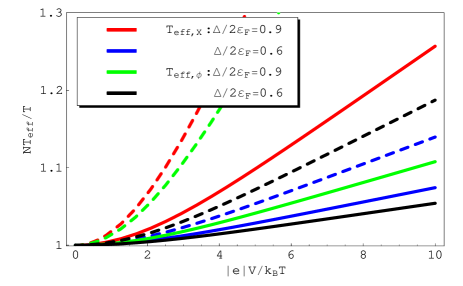
Figure 5: (color online). The effective temperatures $NT_{{\rm eff},X}/T$ and $NT_{{\rm eff},\phi}/T$ as a function of $|e|V/{\rm k}_{\rm B}T$ for $\Delta/2\varepsilon_{\rm F}=0.6$ or $\Delta/2\varepsilon_{\rm F}=0.9$, all at $k_{\rm F}\lambda=1$. The dashed curves are for $P=0$, the solid curves are for $P=0.6$.

The solid curves are obtained for $P=0.6$, the dashed curves do not take into account polarization. Note that the effective temperatures due to current-induced fluctuations can be substantially larger than the actual temperature, and are for large voltage proportional to $|e|V$.

As an application of the effective temperatures derived above, we compute depinning times as a function of the voltage. The effective temperature $T_{\rm eff,X}$ influences depinning from a spatial potential for the domain wall, such as a nanoconstriction. We model the pinning potential by a potential well of width $2\xi$, given by $V=\Delta V(X^{2}/\xi^{2}-1)\theta(|X|-\xi)$ tatara2004 . Using Arrhenius’ law, the escape time is given by $\log(\tau\nu_{0})=N(\Delta V-\hbar F_{X}\xi/\lambda)/{\rm k}_{\rm B}T_{\rm eff,X}$, where $\nu_{0}\sim\Delta V/\hbar$ is the attempt frequency. Note that the effect of the momentum transfer is determined by the ratio $\xi/\Delta V$, and that the force itself is still dependent on the number of spins $N$. We show our results for $\Delta V\lambda/\xi=1$ meV, $N=10$ and several temperatures in Fig. 6. The results for $T_{\rm eff}=T$ are also shown. Note that current-induced fluctuations decrease depinning times with respect to the result with the actual temperature.

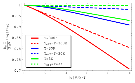
Figure 6: (color online). Logarithm of the escape time $({\rm k}_{\rm B}T/N\Delta V)\log{\tau\nu_{0}}$ as a function of $|e|V/{\rm k}_{\rm B}T$ with (solid curves) and without (dashed curves) current-induced fluctuations. We used $\Delta V\lambda/\xi=1$ meV, $N=10$, $k_{\rm F}\lambda=1$, $\Delta=\varepsilon_{\rm F}$, $P=0$, and several temperatures.

Here, we did not take into account polarization, which reduces this effect since polarization brings down the effective temperature, as was seen in Fig. 5.

IV Discussion

We have established a microscopic theory that describes the effects of current-induced fluctuations on a domain wall. Since fluctuations in the current influence the system via spin transfer and momentum transfer, we find two separate forces, dampings and effective temperatures that correspond to these processes. We note that the ratio of the momentum transfer and the spin transfer $\beta=F_{X}/F_{\phi}$ that we calculate does not yet include the contribution due to spin relaxation. However, this contribution is small compared to the contribution due to momentum transfer when the domain wall is narrow, and can therefore be ignored. In addition to the contribution due to the coupling of the domain wall with the electrons in the leads, that we consider here, there is an intrinsic contribution to the damping due to spin-relaxation, which is of the order $\alpha_{0}\sim 0.01-0.1$ in bulk materials, i.e., of the same order as the voltage-dependent damping parameters that we obtain. A voltage-independent contribution to the damping will decrease the effective temperature, and thereby increase the depinning time somewhat.

As an application, we have studied depinning of the domain wall from a nanoconstriction. The width of the domain wall in nanocontacts is approximately the same as the nanocontact itself bruno1999 . In experiments, it can be as small as $\lambda\sim 1$ nm versluijs2001 ; garcia1999 , which is smaller than the phase coherence length $L_{\phi}\sim 10$ nm in metals at room temperature and therefore permits a Landauer-Büttiker transport approach. Tatara et al. tatara1999 have shown that in nanocontacts in metals Ni and Co, the exchange-splitting energy can reach high values $\Delta/2\varepsilon_{\rm F}\simeq 0.98$. The voltage on the system in the experiment by Coey et al. is of the order $|e|V\sim 0.1$ eV, which leads to $|e|V/{\rm k}_{\rm B}T\simeq 4$ at room temperature. The potential barrier in experiments on nanocontacts for typical displacements $\xi\sim 10\lambda$ versluijs2001 is very large $\Delta V\sim 10$ eV, but can be tuned by applying an external magnetic field. We see from Fig. 6 that at room temperature, the current-induced fluctuations already have an effect on depinning times, even if we take into account the fact that polarization might reduce this effect somewhat. At lower temperatures, this effect becomes larger. Under these circumstances, Coey et al. find no evidence for heating effects, which would be another source of increased fluctuations. Therefore, current-induced fluctuations should be observable with domain walls in nanocontacts.

Depinning of the angle $\phi$ is possible for relatively low values of the transverse anisotropy $K_{\perp}$. This depinning corresponds to switching between Néel walls of different chirality. Between the Néel wall configurations, the domain wall takes the form of a Bloch wall, that has higher energy. Coey et al. coey2001 have argued that in nanoconstrictions, the energy difference is comparable to the thermal energy at room temperature. Now, $T_{{\rm eff},\phi}$ is the effective temperature of interest, and from Fig. 5 we observe that current-induced fluctuations substantially alter this temperature. We therefore expect that effects of current-induced fluctuations on fluctuation-assisted domain-wall transformations can be significant.

This work was supported by the Netherlands Organization for Scientific Research (NWO) and by the European Research Council (ERC) under the Seventh Framework Program. It is a pleasure to thank Henk Stoof for discussions.

References

- (1) A. Einstein, Ann. d. Phys. 17, 549 (1905).
- (2) M.J.M. de Jong and C.W.J. Beenakker, in Mesoscopic Electron Transport, edited by L.L. Sohn, L.P. Kouwenhoven and G. Schoen, NATO ASI Series (Kluwer Academic, Dordrecht, 1997), Vol. 345, pp. 225-258.
- (3) L. Berger, J. Appl. Phys. 55, 1954 (1984).
- (4) P. P. Freitas and L. Berger, J. Appl. Phys. 57, 1266 (1985).
- (5) J.C. Slonczewski, J. Magn. Magn. Mater. 159, L1 (1996).
- (6) L. Berger, Phys. Rev. B. 54, 9353 (1996).
- (7) G. Tatara and H. Kohno, Phys. Rev. Lett. 92, 086601 (2004); 96, 189702 (2006).
- (8) J. Grollier, P. Boulenc, V. Cros, A. Hamzić, A. Vaurès and A. Fert, Appl. Phys. Lett. 83, 509 (2003).
- (9) M. Kläui, C.A.F. Vaz, J.A.C. Bland, W. Wernsdorfer, G. Faini and E. Cambril, Appl. Phys. Lett. 83, 105 (2003).
- (10) A. Yamaguchi, T. Ono, S. Nasu, K. Miyake, K. Mibu and T. Shinjo, Phys. Rev. Lett. 92, 077205 (2004).
- (11) G.S.D. Beach, C. Nistor, C. Knutson, M. Tsoi and J.L. Erskine, Nature Mat. 4, 741-744 (2005).
- (12) M. Yamanouchi, D. Chiba, F. Matsakura, T. Dietl and H. Ohno, Phys. Rev. Lett. 96, 096601 (2006).
- (13) S. Zhang and Z. Li, Phys. Rev. Lett. 93, 127204 (2004).
- (14) M. Hayashi, L. Thomas, C. Rettner, R. Moriya, Y. B. Bazaliy and S.S.P. Parkin, Phys. Rev. Lett. 98, 037204 (2007).
- (15) L. Heyne, M. Klaüi, D. Backes, T.A. Moore, S. Krzyk, U. Rüdiger, L.J. Heyderman, A. Fraile Rodríguez, F. Nolting, T.O. Mentes, M. Á. Niño, A. Locatelli, K. Kirsch and R. Mattheis, Phys. Rev. Lett. 100, 066603 (2008).
- (16) M. Feigenson, J.W. Reiner and L. Klein, Phys. Rev. Lett. 98, 247204 (2007).
- (17) P. Bruno, Phys. Rev. Lett. 83, 2425 (1999).
- (18) J.J. Versluijs, M.A. Bari and J.M.D. Coey, Phys. Rev. Lett. 87, 026601 (2001).
- (19) N. García, M. Muñoz and Y.-W. Zhao, Phys. Rev. Lett. 82, 2923 (1999).
- (20) J. Foros, A. Brataas, Y. Tserkovnyak and G.E.W. Bauer, Phys. Rev. Lett. 95, 016601 (2005).
- (21) A.S. Núñez and R.A. Duine, Phys. Rev. B 77, 054401 (2008).
- (22) A.L. Chudnovskiy, J. Swiebodzinski and A. Kamenev, Phys. Rev. Lett. 101, 066601 (2008).
- (23) J. Foros, A. Brataas, Y. Tserkovnyak and G.E.W. Bauer, cond-mat/08032175.
- (24) H.T.C. Stoof, J. Low Temp. Phys. 114, 11 (1999).
- (25) R.A. Duine, A.S. Núñez and A.H. MacDonald, Phys. Rev. Lett. 98, 056605 (2007).
- (26) A. Mitra and A.J. Millis, Phys. Rev. B 72, 121102(R) (2005).
- (27) I.I. Mazin, Phys. Rev. Lett. 83, 1427 (1999).
- (28) X. Waintal and M. Viret Europhys. Lett. 65, 427 (2004).
- (29) H. Katsura, A.V. Balatsky, Z. Nussinov and N. Nagaosa, Phys. Rev. B 73, 212501 (2006).
- (30) G. Tatara, Y.-W. Zhao, M. Muñoz and N. García, Phys. Rev. Lett. 83, 2030 (1999).
- (31) J.M.D. Coey, L. Berger and Y. Labaye, Phys. Rev. B 64, 020407(R) (2001).