0 [
]The effect of convection on pulsational stability
G. Houdek
Institute of Astronomy, University of Cambridge, Cambridge CB30HA, UK
Abstract
A review on the current state of mode physics in classical pulsators is presented. Two, currently in use, time-dependent convection models are compared and their applications on mode stability are discussed with particular emphasis on the location of the Delta Scuti instability strip.
1 Introduction
Stars with relatively low surface temperatures show distinctive envelope convection zones which affect mode stability. Among the first problems of this nature was the modelling of the red edge of the classical instability strip (IS) in the Hertzsprung-Russell (H-R) diagram. The first pulsation calculations of classical pulsators without any pulsation-convection modelling predicted red edges which were much too cool and which were at best only neutrally stable. What follows were several attempts to bring the theoretically predicted location of the red edge in better agreement with the observed location by using time-dependent convection models in the pulsation analyses (Dupree 1977; Baker & Gough 1979; Gonzi 1982; Stellingwerf 1984). More recently several authors, e.g. Bono et al. (1995, 1999), Houdek (1997, 2000), Xiong & Deng (2001, 2007), Dupret et al. (2005) were successful to model the red edge of the classical IS.
![[Uncaptioned image]](/html/0810.5228/assets/x1.png) Figure 1: Sketch of an overturning hexagonal (dashed lines)
convective cell. Near the centre the gas raises from the
hot bottom to the cooler top (surface) where it moves nearly
horizontally towards the edges, thereby loosing heat. The
cooled gas then descends along the edges to close the circular
flow. Arrows indicate the direction of the flow pattern.
Figure 1: Sketch of an overturning hexagonal (dashed lines)
convective cell. Near the centre the gas raises from the
hot bottom to the cooler top (surface) where it moves nearly
horizontally towards the edges, thereby loosing heat. The
cooled gas then descends along the edges to close the circular
flow. Arrows indicate the direction of the flow pattern.
These authors report, however, that different physical mechanisms are responsible for the return to stability. For example, Bono et al. (1995) and Dupret et al. (2005) report that it is mainly the convective heat flux, Xiong & Deng (2001) the turbulent viscosity, and Baker & Gough (1979) and Houdek (2000) predominantly the momentum flux (turbulent pressure ) that stabilizes the pulsation modes at the red edge.
| Balance between buoyancy & | Kinetic theory of accelerating |
|---|---|
| turbulent drag (Unno 1967, 1977) | eddies (Gough 1965, 1977a) |
| - acceleration terms of convective | - acceleration terms included: , |
| fluctuations neglected | evolve with growth rate |
| - nonlinear terms approximated | - nonlinear terms are neglected |
| by spatial gradients | during eddy growth |
| - neglected in momentum equ. | - included in Eq. (1) |
| - characteristic eddy lifetime: | - determined stochas- |
| tically from parametrized shear | |
| instability | |
| - variation (Unno 1967): | - variation of mixing length |
| according to rapid distortion | |
| theory (Townsend 1976), i.e. | |
| or (Unno 1977): | variation also of eddy shape |
| ( is pressure scale height) | |
| - turbulent pressure neglected | - included in mean |
| in hydrostatic support equation | equ. for hydrostatic support |
2 Time-dependent convection models
The authors mentioned in the previous section used different implementations
for modelling the interaction of the turbulent velocity field
with the pulsation. In the past various time-dependent convection models
were proposed, for example, by Schatzman (1956), Gough (1965, 1977a),
Unno (1967, 1977), Xiong (1977, 1989), Stellingwerf (1982), Kuhfuß (1986),
Canuto (1992), Gabriel (1996), Grigahcène et al. (2005).
Here I shall briefly review and compare the basic concepts of two, currently in
use, convection models. The first model is that by Gough (1977a,b), which
has been used, for example, by Baker & Gough (1979), Balmforth (1992)
and by Houdek (2000). The second model is that by Unno (1967, 1977),
upon which the generalized models by Gabriel (1996) and Grigahcène et al.
(2005) are based, with applications by Dupret et al. (2005).
Nearly all of the time-dependent convection models assume the Boussinesq
approximation to the equations of motion. The Boussinesq approximation relies
on the fact that the height of the fluid layer is small compared with
the density scale height. It is based on a careful scaling argument and
an expansion in small parameters (Spiegel & Veronis 1960; Gough 1969).
The fluctuating convection equations for an inviscid Boussinesq fluid in
a static plane-parallel atmosphere are
| (1) | |||||
| (2) |
supplemented by the continuity equation for an incompressible gas, , where is the turbulent velocity field, is density, is gas pressure, is the acceleration due to gravity, is temperature, is the specific heat at constant pressure, , is the radiative heat flux, is the superadiabatic temperature gradient and is the Kronecker delta. Primes (′) indicate Eulerian fluctuations and overbars horizontal averages. These are the starting equations for the two physical pictures describing the motion of an overturning convective eddy, illustrated in Fig. 1.
In the first physical picture, adopted by Unno (1967), the turbulent element, with a characteristic vertical length , evolves out of some chaotic state and achieves steady motion very quickly. The fluid element maintains exact balance between buoyancy force and turbulent drag by continuous exchange of momentum with other elements and its surroundings. Thus the acceleration terms and are neglected and the nonlinear advection terms provide dissipation (of kinetic energy) that balances the driving terms. The nonlinear advection terms are approximated by and . This leads to two nonlinear equations which need to be solved numerically together with the mean equations of the stellar structure.
The second physical picture, which was generalized by Gough (1965, 1977a,b) to the time-dependent case, interprets the turbulent flow by indirect analogy with kinetic gas theory. The motion is not steady and one imagines the convective element to accelerate from rest followed by an instantaneous breakup after the element’s lifetime. Thus the nonlinear advection terms are neglected in the convective fluctuation equations (1)-(2) but are taken to be responsible for the creation and destruction of the convective eddies (Gough 1977a,b). By retaining only the acceleration terms the equations become linear with analytical solutions and subject to proper periodic spatial boundary conditions, where is time and is the linear convective growth rate. The mixing length enters in the calculation of the eddy’s survival probability, which is proportional to the eddy’s internal shear (rms vorticity), for determining the convective heat and momentum fluxes. Although the two physical pictures give the same result in a static envelope, the results for the fluctuating turbulent fluxes in a pulsating star are very different (Gough 1977a). The main differences between Unno’s and Gough’s convection model are summarized in Table 1.
3 Application on mode stability in Scuti stars
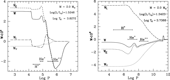
Fig. 2 displays the mode stability of an evolving 1.7 M⊙ Delta Scuti star crossing the IS. The results were computed with the time-dependent, nonlocal convection model by Gough (1977a,b). As demonstrated in the right panel of Fig. 2, the dominating damping term to the work integral for a star located near the red edge is the contribution from the turbulent pressure fluctuations .
Gabriel (1996) and more recently Grigahcène et al. (2005) generalized Unno’s time-dependent convection model for stability computations of nonradial oscillation modes. They included in their mean thermal energy equation the viscous dissipation of turbulent kinetic energy, , as an additional heat source. The dissipation of turbulent kinetic energy is introduced in the conservation equation for the turbulent kinetic energy (e.g. Tennekes & Lumley 1972,3.4; Canuto 1992; Houdek & Gough 1999):
| (3) |
where is the material derivative, is the average (oscillation) velocity, i.e. the total velocity , and is the constant kinematic viscosity (in the limit of high Reynolds numbers the molecular transport term can be neglected). The first and second term on the right of Eq. (3) are the shear and buoyant productions of turbulent kinetic energy, whereas the last term is the viscous dissipation of turbulent kinetic energy into heat. This term is also present in the mean thermal energy equation, but with opposite sign. The linearized perturbed mean thermal energy equation for a star pulsating radially with complex angular frequency can then be written, in the absence of nuclear reactions, as (‘’ denotes a Lagrangian fluctuation and I omit overbars in the mean quantities):
| (4) |
where is the radial mass co-ordinate, and is the total (radiative and convective) luminosity. Grigahcène et al. (2005) evaluated from a turbulent kinetic energy equation which was derived without the assumption of the Boussinesq approximation. Furthermore it is not obvious whether the dominant buoyancy production term, (see Eq. 3), was included in their turbulent kinetic energy equation and so in their expression for .
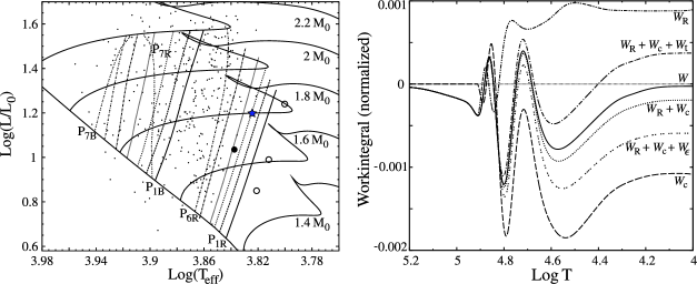
Dupret et al. (2005) applied the convection model of Grigahcène et al. (2005) to Delta Scuti and Doradus stars and reported well defined red edges. The results of their stability analysis for Delta Scuti stars are depicted in Fig. 3. The left panel compares the location of the red edge with results reported by Houdek (2000, see also Fig. 2) and Xiong & Deng (2001). The right panel of Fig. 3 displays the individual contributions to the accumulated work integral for a star located near the red edge of the mode (indicated by the ‘star’ symbol in the left panel). It demonstrates the near cancellation effect between the contributions of the turbulent kinetic energy dissipation , , and turbulent pressure, , making the contribution from the fluctuating convective heat flux, , the dominating damping term. The near cancellation effect between and was demonstrated first by Ledoux & Walraven (1958, 65) (see also Gabriel 1996) by writing the sum of both work integrals as:
| (5) |
where is the stellar mass, is the enclosed mass at the bottom of the envelope and ( is specific entropy) is the third adiabatic exponent. Except in ionization zones and consequently .
The convection model by Xiong (1977, 1989) uses transport equations for the second-order moments of the convective fluctuations. In the transport equation for the turbulent kinetic energy Xiong adopts the approximation by Hinze (1975) for the turbulent dissipation rate, i.e. , where is the Heisenberg eddy coupling coefficient and is the wavenumber of the energy-containing eddies. However, Xiong does not provide a work integral for (neither does Unno et al. 1989, 26,30) but includes the viscous damping effect of the small-scale turbulence in his model. The convection models considered here describe only the largest, most energy-containing eddies and ignore the dynamics of the small-scale eddies lying further down the turbulent cascade. Small-scale turbulence does, however, contribute directly to the turbulent fluxes and, under the assumption that they evolve isotropically, they generate an effective viscosity which is felt by a particular pulsation mode as an additional damping effect. The turbulent viscosity can be estimated as (e.g. Gough 1977b; Unno et al. 1989, 20) , where is a parameter of order unity. The associated work integral can be written in Cartesian co-ordinates as (Ledoux & Walraven 1958, 63)
| (6) |
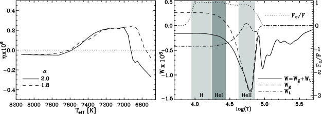
where and is the displacement eigenfunction. Xiong & Deng (2001, 2007) modelled successfully the IS of Delta Scuti and red giant stars and found the dominating damping effect to be the turbulent viscosity (Eq. 6). This is illustrated in Fig. 4 for two Delta Scuti stars: one is located inside the IS (left panel), the other outside the cool edge of the IS (right panel). The contribution from the small-scale turbulence was also the dominant damping effect in the stability calculations by Xiong et al. (2000) of radial p modes in the Sun, although the authors still found unstable modes with orders between . The importance of the turbulent damping was reported first by Goldreich & Keeley (1977) and later by Goldreich & Kumar (1991), who found all solar modes to be stable only if turbulent damping was included in their stability computations. In contrast, Balmforth (1992), who adopted the convection model of Gough (1977a,b), found all solar p modes to be stable due mainly to the damping of the turbulent pressure perturbations, , and reported that viscous damping, , is about one order of magnitude smaller than the contribution of . Turbulent viscosity (Eq. 6) leads always to mode damping, where as the perturbation of the turbulent kinetic energy dissipation, (see Eq. 4), can contribute to both damping and driving of the pulsations (Gabriel 1996). The driving effect of was shown by Dupret et al. (2005) for a Doradus star.
4 Summary
We discussed three different mode stability calculations of Delta Scuti stars which successfully reproduced the red edge of the IS. Each of these computations adopted a different time-dependent convection description. The results were discussed by comparing work integrals. All convection descriptions include, although in different ways, the perturbations of the turbulent fluxes. Gough (1977a), Xiong (1977, 1989), and Unno et al. (1989) did not include the contribution to the work integral because in the Boussinesq approximation (Spiegel & Veronis 1960) the viscous dissipation is neglected in the thermal energy equation. In practise, however, this term may be important. Grigahcène et al. (2005) included but ignored the damping contribution of the small-scale turbulence , which was found by Xiong & Deng (2001, 2007) to be the dominating damping term. The small-scale damping effect was also ignored in the calculations by Houdek (2000). A more detailed comparison of the convection descriptions has not yet been made but Houdek & Dupret have begun to address this problem.
Acknowledgements.
I am grateful to Douglas Gough for helpful discussions and to the HelAs organizing committee for travel support. Support by the UK Science and Technology Facilities Council is acknowledged. ReferencesBaker N., Gough D.O. 1979, ApJ, 234, 232 Balmforth N.J. 1992, MNRAS, 255, 603 Bono G., Caputo F., Castellani V., et al. 1995, ApJ, 442, 159 Bono G., Marconi M., Stellingwerf R. 1999, ApJSS, 122, 167 Canuto V. 1992, ApJ, 392, 218 Dupree R.G. 1977, ApJ, 215, 232 Dupret M.-A., Grigahcène A., Garrido R., et al. 2005, A&A, 435, 927 Gabriel M. 1996, Bull. Astron. Soc. India, 24, 233 Goldreich P., Keeley D.A. 1977, ApJ, 211, 934 Goldreich P., Kumar P. 1991, ApJ, 374, 366 Gonzi G. 1982, A&A, 110, 1 Gough D.O. 1965, in Geophys. Fluid Dynamics, Woods Hole Oceanographic Institutions, Vol. 2, Woods Hole, Mass., p. 49 Gough D.O. 1969, J. Atmos. Sci., 26, 448 Gough D.O. 1977a, ApJ, 214, 196 Gough D.O. 1977b, in Problems of Stellar Convection, Spiegel E.A., Zahn J.-P., eds, Springer-Verlag, Berlin, p. 15 Grigahcène A., Dupret M.-A., Gabriel M., et al. 2005, A&A, 434, 1055 Hinze J.O. 1975, Turbulence, McGraw-Hill, New York Houdek G. 1997, in Proc. IAU Symp. 181: Sounding Solar and Stellar Interiors, Schmider F.-X., Provost J., eds, Nice Observatory, p. 227 Houdek G. 2000, in Delta Scuti and Related Stars, Breger M., Montgomery M.H., eds, ASP Conf. Ser., Vol. 210, Astron. Soc. Pac., San Francisco, p. 454 Houdek G., Gough D.O. 1999, in Theory & Tests of Convection in Stellar Structure, Guinan E.F., Montesinos B., eds, ASP Conf. Ser. 173, San Francisco, p. 237 Kuhfuß R. 1986, A&A, 160, 116 Ledoux P., Walraven T. 1958, in Handbuch der Physik, Vol. LI, Flügge S., ed., Springer-Verlag, Berlin, p. 353 Schatzman E. 1956, Annales d’Astrophysique, 19, 51 Spiegel E.A., Veronis G. 1960, ApJ, 131, 442 (correction: ApJ, 135, 665) Stellingwerf R.F. 1982, ApJ, 262, 330 Stellingwerf R.F. 1984, ApJ, 284, 712 Tennekes H., Lumley J.L. 1972, A First Course in Turbulence, The MIT Press Townsend A.A. 1976, The Structure of Turbulent Shear Flow, CUP Unno W. 1967, PASJ, 19, 40 Unno W. 1977, in Problems of Stellar Convection, Spiegel E.A., Zahn J.-P., eds, Springer-Verlag, Berlin, p. 315 Unno W., Osaki Y., Ando H., Saio H, Shibahashi H. 1989, Nonradial Oscillations of Stars, Second Edition, University of Tokyo Press Xiong D.R. 1977, Acta Astron. Sinica, 18, 86 Xiong D.R. 1989, A&A, 209, 126 Xiong D.R., Cheng Q.L., Deng L. 2000, MNRAS, 319, 1079 Xiong D.R., Deng L. 2001, MNRAS, 324, 243 Xiong D.R., Deng L. 2007, MNRAS, 378, 1270