Multiplexing of discrete chaotic signals in presence of noise

Abstract

In this paper, multiplexing of discrete chaotic signals in the presence of noise is investigated. Existing methods are based on chaotic synchronization which is susceptible to noise and parameter mismatch. Furthermore, these methods fail for multiplexing more than two discrete chaotic signals. We propose two novel methods to multiplex multiple discrete chaotic signals based on the principle of symbolic sequence invariance in the presence of noise and finite precision implementation of finding the initial condition of an arbitrarily long symbolic sequence of a chaotic map.

I Motivation

In this paper, we investigate multiplexing of chaotic signals in the presence of noise. The fact that chaotic signals have a lot of redundancy in them is exploited here. We first motivate the application and then provide new methods.

Multiplexing of signals is a very important requirement in most communication systems. Consider the scenario where there are multiple signals from multiple senders to be transmitted to multiple receivers, but there exists only one communication channel that can transmit only one signal at any given time. In such a scenario, it would be beneficial if all the signals are “added” in a special way to create a single composite signal for transmission across the communication channel. This single composite signal is “separated” to the respective signals in a lossless fashion at the other end of the channel. Note that there is also noise which is invariably added at the channel. This scenario can also occur in transmission of neuronal signals from different parts of the brain to various parts of the body through a single channel.

For linear communication systems, standard ways such as frequency division multiplexing (different signals are allocated different parts of the frequency spectrum) and time division multiplexing (different signals are allocated different time slots for transmission) are used to increase the information capacity of the channel GibsonBook . Nonlinear chaotic oscillators are increasingly being used in communications since it offers a potential advantage over conventional classical methods in terms of noise performance Multiplex1 . Multi-user chaotic communications has become a hot topic of research in recent times Multiplex2 . It is also potentially useful in spectrum-spreading communication systems. Hence there is a need for multiplexing chaotic signals.

II Existing work and their limitations

There has been some work in multiplexing chaotic signals. For the first time in 1996, multiplexing of chaos using chaotic synchronization was investigated in a simple map and an electronic circuit model by Tsimring and Sushchik Multiplex3 . Liu and Davis Multiplex4 used a scalar signal to simultaneously synchronize two different pairs of chaotic oscillators. They called this method as dual synchronization. However, there are several limitations of this method. They derive a condition for dual synchronization which holds only for certain discrete chaotic signals (maps) and for certain values of the coupling coefficients. The notable omission is the binary map (Bernoulli shift). They show that the binary map does not satisfy the condition for dual synchronization for any value of the coupling coefficients. Thus, chaotic signals from the binary map can’t be multiplexed by their method. Another limitation is that their method can only work with two chaotic signals. It is not known whether the method can be extended to multiple signals (more than two) from different maps.

There has been more work in multiplexing chaotic signals from continuous chaotic systems (flows). Liu and Davis Multiplex4 extend their work to multiplex signals from delay-differential equations. Further progress has been made by Di Ning et. al. Multiplex5 who extend Liu’s method for 3D continuous chaotic systems (Lorenz and Rössler systems). This has been further improved by Salarieh and Shahrokhi Multiplex6 who make use of a time-varying output feedback strategy to achieve dual synchronization without the need for all the master states (only a linear combination of the master states are enough).

All the developments were only for two chaotic systems until the work of Salarieh and Shahrokhi Multiplex7 who succeeded in multiplexing more than two continuous chaotic signals using chaotic synchronization via output feedback strategy. They derive a necessary condition for multi-synchronization and demonstrate the algorithm to the Chen-Lorenz-Rossler and the Duffing-Van der Pol continuous time chaotic dynamical systems. However, none of these methods work for multiple discrete chaotic signals. Another serious limitation is that chaotic synchronization is susceptible to noise and to parameter mismatch. Even one percent of parameter mismatch leads to $8\%$ of synchronization error and one percent of noise results in a synchronization error of $4\%$ as reported by Multiplex4 .

Vaidya’s method Vaidya-noise-restent which multiplexes more than two discrete chaotic signals remains as the latest development on multiplexing chaotic signals from discrete chaotic signals (1D maps). Vaidya’s method does not use chaotic synchronization and is fundamentally different from the previous approaches. We will describe the method and its drawbacks in Section III.3 since we are going to use some of the ideas from this method to improve upon it. In principle, it is possible to extend the methods that is proposed in this paper to flows and to higher dimensional chaotic dynamical systems, but these will not be pursued here. Since Liu and Davis’ method does not work for the standard binary map, we shall consider chaotic signals from the standard binary map with randomly chosen initial conditions.

II.1 New Approach

Our approach considers two different scenarios as shown in Figure 1. In Scenario 1, the communicating channel is noisy and there is no control on the noise that is added during transmission of the signal (Figure 1(a)). However, it shall be assumed that the magnitude of the noise is limited (we shall give conditions on the magnitude of noise that is allowed by our methods). The noise is uniformly distributed. The signals are chaotic and the noise that is added during transmission is uncontrolled but limited in magnitude.

In Scenario 2 (Figure 1(b)), the communication channel is lossless, but the noise is added at the sender. The noise is assumed to be of the same magnitude as the chaotic signals and uniformly distributed. But the way the noise is added is under control. This scenario corresponds to steganography  or cryptographic applications where the noise could be the “payload” to be secretly transmitted.

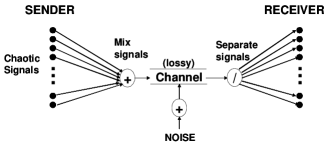
(a) Scenario 1: Channel is lossy, noise is additive and limited in magnitude (Methods 1 and 2).

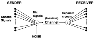
(b) Scenario 2: Channel is lossless, but noise which has the same magnitude as the signal, is added in a special way at the sender (Method 3).

Figure 1: Multiplexing of chaotic signals in the presence of noise.

Recently, Vaidya Vaidya-noise-restent suggested a novel multiplexing algorithm for 1D discrete chaotic signals in the presence of noise. We shall call this as Method 1 and review it briefly and list some of its limitations. A new method (Method 2) will be proposed which overcomes some of the limitations of Method 1. Both these methods are solutions to Scenario 1. A novel method (Method 3) is proposed for Scenario 2.

III Method 1: Vaidya’s Noise Resistant Map

Vaidya’s method Vaidya-noise-restent is a solution to multiplexing of chaotic signals in the presence of noise (Scenario 1) which does not make use of chaotic synchronization like the previous approaches. Vaidya proposes a noise-resistant version of the Tent map. Since we are going to deal mainly with the standard binary map, a minor modification leads to a noise-resistant version of the binary map. It is given by the following set of equations:

$$y = 2x,~{}~{}~{}~{}~{}~{}~{}~{}~{}~{}~{}~{}0\leq x<\frac{p}{2}$$

$$= 2x+q,~{}~{}~{}~{}~{}~{}~{}~{}~{}~{}~{}~{}\frac{p}{2}\leq x<p$$

$$= 0,~{}~{}~{}~{}~{}~{}~{}~{}~{}~{}~{}~{}~{}~{}~{}p\leq x<p+q$$

$$= 2x-2(p+q),~{}~{}~{}~{}~{}~{}p+q\leq x<\frac{3p}{2}+q$$

$$= 2x-(2p+q),~{}~{}~{}~{}~{}~{}\frac{3p}{2}+q\leq x<2p+q$$

$$= 0,~{}~{}~{}~{}~{}~{}~{}~{}~{}~{}~{}~{}~{}~{}~{}2p+q\leq x<1.$$

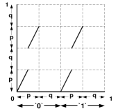
Figure 2: $T_{noiseres}$: Noise-resistant Binary Map.

Figure 2 depicts the noise resistant binary map (denoted by $T_{noiseres}$). Vaidya establishes that there exists a conjugacy between the ordinary binary map and $T_{noiseres}$. Given any chaotic signal on the binary map (a chaotic signal is trajectory on the map for a given initial condition), one can find the equivalent signal on $T_{noiseres}$. $p$ ($0<p\leq 0.5$) and $q$ ($0\leq q<0.5$) can be chosen such that $2p+2q=1$.

The symbolic sequence is defined as follows:

$$S(x_{i}) = 0,~{}~{}~{}~{}~{}~{}0\leq x_{i}<p+q$$

$$= 1,~{}~{}~{}~{}~{}~{}p+q\leq x_{i}<1.$$

Here, $X=\{x_{i}\}_{i=1}^{i=m}$ is the chaotic trajectory (or chaotic signal) starting from an initial condition $x_{1}$. $S(X)$ denotes the symbolic sequence for the entire trajectory.

III.1 Noise-resistance

For any given chaotic signal $X$ on $T_{noiseres}$, if noise $N=\{n_{i}\}_{i=1}^{i=m}$ is added such that each $n_{i}$ satisfies $0\leq n_{i}<q$, then it can be seen that the symbolic sequence remains unchanged:

$$S(X)=S(X+N).$$ (1)

The signal $X$ is transmitted at the sender and the resulting signal $Z=X+N$ is what is received at the receiver. However, because of the above property of symbolic sequence invariance, we can compute $S(X)$ (=$S(Z)$) and iterating backwards on the map, we can find the initial condition $x_{1}$. Knowing $x_{1}$, we can easily compute $x_{2},\ldots,x_{m}$ and thus we can recover $X$ losslessly. Furthermore, we can also compute $N=Z-X$ accurately. Thus we have recovered both the original chaotic signal and the noise. This noise resistance property is provided by a non-zero value of $q$. The larger the $q$, the higher is the resistance to noise but at the same time the length of the signal has to be longer in order to determine the initial condition $x_{1}$ accurately from the symbolic sequence.

III.2 Cascading Noise-resistant Maps

Vaidya goes one step further and defines a cascade of such noise-resistant maps. To add another chaotic signal $Y$ to $X$, Vaidya defines a similar noise-resistant map which maps $[0,q)$ onto itself. It is self-similar to $T_{noiseres}$. Thus, he defines a whole cascade of noise-resistant maps, all of which are self similar to the original one. The domain of succeeding maps reduces exponentially. For further details, please refer to Vaidya-noise-restent .

With these cascade of maps, one could now add a whole family of chaotic signals $\{X_{1},X_{2},\ldots,X_{k}\}$ to one noise signal $N$ (on the channel) with magnitude dictated by the number of maps, to yield the signal $Z$. The symbolic sequence invariance is maintained at each step of cascading. Thus, the symbolic sequence of $Z$ is used to decode $X_{1}$ and $N_{1}$ where $N_{1}$ is the sum of $\{X_{2},X_{3},\ldots,X_{k}\}$ and $N$. The symbolic sequence of $N_{1}$ is the same as that of $X_{2}$ and hence $X_{2}$ can be decoded. This procedure is repeated until all the signals are losslessly recovered along with $N$. Vaidya successfully applies this method to multiplex 100 chaotic signals.

III.3 Drawbacks of Method 1

The drawbacks of Method 1 are as follows:

1. Given chaotic signals from various chaotic maps, one has to find the corresponding signals in the noise-resistant binary/tent map using topological conjugacy. This is cumbersome and although we can have a finite precision implementation of the chaotic maps and the noise-resistant binary map, it is difficult to develop finite precision implementation of the topological conjugacy. For example, if the signal $X$ is from the logistic map, then the topological conjugacy will involve trigonometric functions which would have to be expressed as truncated infinite series. This may lead to errors in the recovery of $X$.

2. The amount of noise that can be added reduces exponentially as the number of chaotic signals to be multiplexed increases linearly.

3. It is in principle possible to extend the idea of noise resistant maps to other chaotic maps like the logistic map. However, for each new map, the equations have to be worked out explicitly.

We are motivated to invent new methods of multiplexing which will circumvent the above problems. While exploiting the idea of symbolic sequence invariance under the addition of noise, we would like to devise a method which will work for any 1D chaotic unimodal map (and generalizable to other kinds of maps and higher dimensional ones) without the necessity of topological conjugacy. The scenario where the magnitude of noise is equal to that of the signal also needs to be addressed.

IV Method 2

The key idea of Method 1 is the notion of symbolic sequence invariance. As long as we ensure that the symbolic sequence of the original chaotic signal $X$ is unaffected by adding the noise $N$ (uniformly distributed), the resulting signal $Z=X+N$ has the same symbolic sequence as $X$ ($S(Z)=S(X)$). Then, given this arbitrarily long symbolic sequence $S(X)$, the problem reduces to determining its initial condition and iterating this initial condition to obtain the entire chaotic signal $X$. Once $X$ is determined, one could subtract $X$ from $Z$ to obtain the noise signal $N$.

In order to find the initial condition from an arbitrarily long symbolic sequence of a chaotic map, we make use of GLS-coding. Generalized Luröth Series or GLS-coding for short, is a new entropy coding algorithm NithinGLS that achieves the Shannon’s entropy rate for lossless data compression. The idea of GLS-coding is to first embed the stochastic (binary) i.i.d source into the appropriate GLS and then treating the message as a symbolic sequence, the initial condition is determined by a backward iteration. A finite precision implementation of GLS-coding is described in the Appendix. Using such an implementation, it is possible to determine accurately the initial condition of an arbitrarily long symbolic sequence. Our implementation is for the skew-tent and skew-binary maps and can be extended to other maps. The standard tent map and binary map are part of this family.

The algorithm for Method 2 is described as follows:

1. Let $X_{1},X_{2},\ldots X_{k}$ be $k$ chaotic signals of length $m$ to be multiplexed. Each of these signals are obtained from distinct initial conditions (randomly chosen) on the standard binary map.

2. Compute the symbolic sequence $\{SX_{i}\}_{i=1}^{i=k}=\{S(X_{i}(1)),S(X_{i}(2)),\ldots S(X_{i}(m))\}_{i=1}^{i=k}$. The function S(.) is defined as follows:

   $$S(x) = 0,~{}~{}~{}~{}~{}~{}0\leq x<0.5$$ (2)

   $$= 1,~{}~{}~{}~{}~{}~{}0.5\leq x<1.$$

3. Compute $\{S_{i}\}_{i=1}^{i=m}$ $=$ $\{<$ $SX_{1}(1)$$SX_{2}(1)$$\ldots$ $SX_{k}(1)$$>_{2}$, $<SX_{1}(2)SX_{2}(2)$$\ldots SX_{k}(2)>_{2}$ $\ldots<SX_{1}(m)SX_{2}(m)$$\ldots SX_{k}(m)>_{2}\}$. Here, $<.>_{B}$ denotes a number that is base-$B$ representation.

4. Compute $D=\{D_{i}\}_{i=1}^{i=m}$ where $D_{i}=<S_{i}>_{10}$.

5. Compute $Z=\{Z_{i}\}_{i=1}^{i=m}$ where $Z_{i}=\frac{2D_{i}+1}{2^{k+1}}$.

6. Transmit $Z$ across the channel.

7. Receive $Z_{noisy}=Z+N$. Here $N=\{N_{i}\}_{i=1}^{i=m}$ where each $N_{i}$ is uniformly distributed noise in the range $(-2^{-(k+1)},+2^{-(k+1)})$.

8. At receiver, compute $D_{noisy}=\lfloor 2^{k}Z_{noisy}\rfloor$ where $\lfloor(.)\rfloor$ is the floor operation which computes the maximum integer that is less than the argument. Note that $D_{noisy}=D$. This is because $D<2^{k}Z_{noisy}<(D+1)$. The floor operator makes this equal to $D$ since $D$ is always a positive integer. This is where we have made use of the fact that the symbolic sequence is invariant in spite of noise. Here $D$ has the information of the symbolic sequence of all the $k$ chaotic signals.

9. Once we have $D_{noisy}=D$, we can recover the symbolic sequences of each of the $k$ chaotic signals and thereby recover the $k$ initial conditions $\{X_{1}(1),X_{2}(1),\ldots,X_{k}(1)\}$ by GLS-coding (see Appendix).

10. From the initial conditions, the $k$ chaotic signals can be recovered.

11. The noise signal can be recovered at the receiver by computing $Z$ from $D$ and computing $N=Z_{noisy}-Z$.

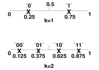
Figure 3: Method 2: For the cases $k=1$ and $k=2$. The points marked ‘$X$’ are transmitted depending on the symbolic sequences of the chaotic signals. Owing to noise at the channel, the received signal will also be uniformly distributed in the range $[0,1)$. This explains Figure 5(c).

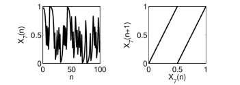
Figure 4: Method 2: Multiplexing of $k=10$ chaotic signals in the presence of one noise signal $N$ – (a) Top left: The 7th Chaotic Signal $X_{7}(.)$. $m=1000$, but only first 100 shown, (b) Top right: Phase Portrait of $X_{7}(.)$, (c) Bottom: Histogram of $X_{7}(.)$.

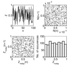
Figure 5: Method 2: Multiplexing of chaotic signals in the presence of noise –(a) Top left: $Z$ signal (showing first 100 values only), (b) Top right: Phase portrait of noise signal $N$, (c) Bottom left: Phase portrait of $Z_{noisy}$, (d) Bottom right: Histogram of $Z_{noisy}$.

IV.1 Experimental Simulations

As a simple example, Figure 3 shows the points transmitted for the case $k=1$ and $k=2$.

Method 2 was experimentally simulated for $k=10$ chaotic signals of length $m=1000$ each. They were all generated by randomly chosen initial conditions on the standard binary map. Figure 4 shows the seventh chaotic signal $X_{7}$. The phase portrait and the histogram are also shown. Figure 5 shows $Z$, the phase portrait of noise signal $N$, phase portrait of $Z_{noisy}$ after the addition of noise and the histogram of $Z_{noisy}$. All the 10 chaotic signals and the noise signal were successfully recovered in a lossless fashion at the receiver. We have used the finite precision implementation of GLS-coding as proposed in Appendix. This confirms the efficacy of Method 2.

V Method 3

The biggest advantage of Method 2 is that in principle it works for any dynamical system. As long as we know the Markov partitions of the dynamical system, we can define the symbolic sequence and hence use Method 2. There is no need of using topological conjugacy or construction of special noise-resistant maps like Method 1. However, one needs to develop an analog of GLS-coding (i.e. finding initial condition for an arbitrary long symbolic sequence of the dynamical system as given in Algorithm 1 in Appendix) for the method to work.

Method 2 works in the presence of a lossy channel, the noise being additive, but the magnitude of noise that is tolerated depends on the number of signals being multiplexed. As the number of signals ($k$) increases, the magnitude of noise ($2^{-k}$) that can be tolerated at the channel, goes down exponentially. Method 3 overcomes this limitation. The noise magnitude can be equal to the signal. However, we can no longer operate in Scenario 1. We assume that we have control on the “way” the noise is added (noise is still assumed to be uniformly distributed) and that the channel is lossless (Scenario 2).

Method 3 is described as follows:

1. Let $X_{1},X_{2},\ldots X_{k}$ be $k$ chaotic signals of length $m$ to be multiplexed. Each of these signals are obtained from distinct initial conditions on the standard binary map.

2. Let noise signal be $N=\{N_{i}\}_{i=1}^{i=m}$ where each $N_{i}$ is independent and identically distributed (uniform) in the range $(0,1)$. Noise signal $N$ is independently generated but available at the receiver.

3. Given two signals $A=\{A(i)\}_{i=1}^{i=m}$ and $B=\{B(i)\}_{i=1}^{i=m}$ where $A$ is a chaotic signal ($B$ can be anything), we define the operation $A+B.S(A)=\{A(i)+B(i).S(A(i))\}_{i=1}^{i=m}$ as follows:

   $$A(i)+B(i).S(A(i)) = A(i)-B(i),~{}~{}~{}\textrm{~{}if~{}}S(A(i))=0$$

   $$= A(i)+B(i),~{}~{}~{}\textrm{~{}if~{}}S(A(i))=1.$$

   where $S(.)$ is defined in Equation 2.

4. Compute the following signals:

   $$Z_{1} = \frac{X_{1}+N.S(X_{1})+1}{3}$$

   $$Z_{2} = \frac{X_{2}+Z_{1}.S(X_{2})+1}{3}$$

   $$Z_{3} = \frac{X_{3}+Z_{2}.S(X_{3})+1}{3}$$

   $$\vdots$$

   $$Z_{k} = \frac{X_{k}+Z_{k-1}.S(X_{k})+1}{3}$$

   $$Z = Z_{k}.$$

5. Transmit $Z$ on the lossless channel. Note that the dynamic range of $Z$ is $[0,1)$.

6. Receiver receives $Z$. By symbolic sequence invariance, we have the following identities:

   $$S(Z)=S(Z_{k}) = S(X_{k})$$

   $$S(Z_{k-1}) = S(X_{k-1})$$

   $$\vdots$$

   $$S(Z_{1}) = S(X_{1}).$$

7. We start with $Z$ and compute $S(Z_{k})$. By the first identity, we have $S(X_{k})$. GLS-coding is applied to determine $X_{k}(1)$. Hence $X_{k}$ is recovered losslessly. Knowing $X_{k}$ and $S(X_{k})$, we can compute $Z_{k-1}$ by the following equations:

   $$Z_{k-1}(i) = X_{k}(i)-3Z(i)+1,~{}~{}~{}\textrm{~{}if~{}}S(X_{k}(i))=0$$

   $$= 3Z(i)-X_{k}(i)-1,~{}~{}~{}\textrm{~{}if~{}}S(X_{k}(i))=1.$$

8. Knowing $Z_{k-1}$, we repeat the procedure to extract $X_{k-1}$ and $Z_{k-2}$. This is repeated until we have extracted all the chaotic signals and the noise signal $N$. Note that noise can be thought of as $Z_{0}$ and the same procedure applies.

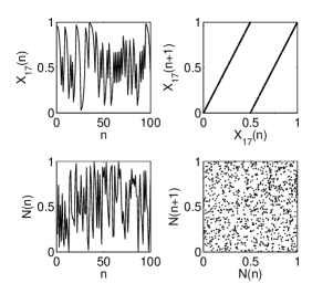
Figure 6: Method 3: Multiplexing of $k=24$ chaotic signals in the presence of one noise signal – (a) Top left: The 17th Chaotic Signal $X_{17}(.)$. The length $m=1000$, but only the first 100 shown, (b) Top right: Phase Portrait of $X_{17}(.)$, (c) Bottom left: Noise signal $N(.)$, (d) Bottom right: Phase Portrait of $N(.)$. Note that magnitude of $N$ is the same as that of $X$.

V.1 Experimental Simulations

Method 3 was experimentally simulated for $k=24$ chaotic signals of length $m=1000$ each and one noise signal of the same length. The chaotic signals were all generated by randomly chosen initial conditions on the standard binary map. Figure 6(a) shows the 17th chaotic signal $X_{17}$. The phase portrait is shown in Figure 6(b). Figure 6(c) shows the noise signal $N$ which has the same magnitude as that of the chaotic signal. The phase portrait of noise signal $N$ is shown in Figure 6(d). The final signal that is transmitted on the lossless channel $Z$ is shown in Figure 7(a). Its phase portrait and histogram are shown in Figure 7(b) and (c) respectively. Note that in this method, the final signal $Z$ does not have uniform distribution although the individual chaotic signals and the noise signals are uniform. This is because of the special way in which the signals were added.

All the 24 chaotic signals and the noise signal were successfully recovered in a lossless fashion at the receiver. We have used the finite precision implementation of GLS-coding as proposed in Appendix. This confirms the efficacy of Method 3.

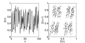
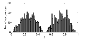
Figure 7: Method 3: Multiplexing of chaotic signals in the presence of noise – (a) Top left: $Z$ signal generated by Method 3 is not uniformly distributed. This is transmitted on the lossless channel, (b) Top right: Phase portrait of $Z$, (c) Bottom: Histogram of $Z$ showing that it is bimodal.

VI Remarks on the Three Methods

The following observations can be made on the three methods:

1. The idea of symbolic sequence invariance is the key to the success of all the three methods. The way this idea is implemented is different in the three methods.

2. The way noise is handled is the same in Methods 1 and 2 since there is no control on the noise in Scenario 1. Scenario 2 is much more restrictive in terms of noise.

3. All the three methods rely on the finite precision implementation of GLS-coding, i.e. finding the initial condition given an arbitrarily long symbolic sequence of the chaotic signal (refer to Appendix). The method of extracting the symbolic sequence from a “noisy non-linear system” and performing GLS-coding is analogous to filtering out noise in linear systems by means of integration or other linear filters (for eg., low pass filters).

4. Methods 2 and 3 can be easily extended to tent map, skew-tent map, logistic map and other unimodal maps. It is also possible to extend the methods to non-unimodal 1D maps and possibly higher dimensional maps. The key is to find an analog of GLS-coding in those cases, which we believe is possible.

5. Method 1 has a hint of using the idea of ‘forbidden symbol’ Boyd1997 ; ARQ ; GrangettoForbiddenSymbol ; TrellisAC by allocating the length $q$ on the interval which is never used by the map. This method can be potentially used for error correction and detection.

6. In Method 2, just by observing the signal on the channel, no information can be gleaned. The distribution is uniform and the phase portrait is also random looking. The fact that multiple chaotic signals have been embedded is not obvious. This property enables it to be used in steganography or information hiding. In LSB-steganography, the Least Significant Bit (LSB) of natural signals is replaced by the secret (noise or noise-like). Method 2 is doing the reverse: MSB-steganography, where the Most Significant Bit (MSB) of the secret (noise or noise-like) is replaced by the symbolic sequence of the chaotic signal.

7. Method 3 can handle any number of chaotic signals and one noise signal. However, in practice there will be limitation on the number of signals owing to finite precision since we are rescaling the range of the signals to $[0,1)$ (by addition of 1 and division by 3).

8. The methods show that chaotic signals are highly redundant and hence robust to noise. As long as the symbolic sequence is preserved, the actual signal can be distorted to a great deal. Also, forward iteration of chaotic dynamical systems exhibits sensitive dependence on initial conditions, but backward iteration shows resistance to noise. These features are not exhibited by random/stochastic signals. This probably makes a strong case for why biological systems may use chaotic signals for transmission of information. Neuronal signals may use similar mechanism for robust transport of information.

9. The above methods will not work for purely random signals or for non-chaotic signals since there is no way we can construct the entire trajectory by knowing the symbolic sequence. The redundancy of chaotic signals is necessary. At the same time, chaotic signals appear “random” in distribution.

10. In contrast with earlier work on multiplexing discrete chaotic signals using chaotic synchronization, our methods can multiplex more than two discrete chaotic signals. There are no coupling coefficients used in our methods and hence there is no condition to be satisfied for multiplexing. As noted previously, earlier methods based on chaotic synchronization are vulnerable to noise and parameter mismatch. Our methods are completely robust to any amount of parameter mismatch since our methods do not rely on chaotic synchronization. Methods 1 and 2 can tolerate noise but limited by the number of signals that is added. However, in Method 3, the noise magnitude is the same as that of the signals.

11. The methods that we have developed can be potentially used in communication protocols, cryptography and steganography applications.

12. There is no violation of Shannon’s theorems for information transmission in any of the methods. By transmitting the entire trajectory, we are sending lots of bits, much more than actually required for sending only the initial condition. These methods are not meant for compression of data. These are mechanisms to exploit the inherent redundancy in chaotic signals in spite of noise.

VII Conclusions and Open Problems

In this work, GLS-coding was used for multiplexing of chaotic signals in the presence of noise. By using the idea of symbolic sequence invariance, we were able to “add” several chaotic signals and “separate” them losslessly at the receiver. We can either have a lossy channel but with limited noise (Methods 1 and 2) or have a lossless channel with noise having the same magnitude as the signal “added” in a very special way at the sender (Method 3). An open problem is to investigate whether one can have both features in a single method.

The inherent redundancy and structure in chaotic signals which otherwise appear random in probability distribution can be harnessed for robust communication of information. It is quite likely that such efficient mechanisms (or similar ones) of handling noise in dynamical systems are already being employed in naturally occurring physical and biological systems.

Compared to existing methods of multiplexing discrete chaotic signals, our methods are significantly superior in all respects. The newly proposed methods can handle multiple signals from multiple maps (including Bernoulli shift or the binary map which was not possible by the method of Liu and Davis), completely robust to parameter mismatch and good noise resistance capability.

Appendix: Finite Precision Implementation of GLS-coding

The idea of GLS-coding NithinGLS is to first embed the stochastic (binary) i.i.d source into the appropriate GLS and then treating the message as a symbolic sequence, the initial condition is determined by a backward iteration. This actually results in an interval (since the symbolic sequence is finite in length) and the mid-point of the interval is used as the initial condition. As the length of the symbolic sequence increases, the interval in which the initial condition is going to lie shrinks in size. This creates problem in performing the backward iteration on a finite precision computer as the two ends of the interval come very close to each other and at some point it would be no longer possible to continue with the backward iteration. This problem needs to be addressed by some kind of re-normalization or re-scaling of the interval, in order for the method to be useful for encoding long sequences. Another problem with the method is that there is a long encoding delay. No output can be written/sent unless the entire initial condition is determined, which happens only after all the input bits are encoded. Luca’s chaotic compression method Luca also has similar problems but is not addressed by them.

There has been efforts to address both these problems for Arithmetic Coding Langdon1981 . Since GLS-coding is an extension of Arithmetic Coding, these methods could be used.

The idea is as follows. As soon as the interval completely lies to the left of $p$ (for the standard tent map and binary map, $p=0.5$), the final initial condition will have a ‘0’ in its binary expansion (‘1’ if the interval is completely to the right of $p$). Hence, this can be written as output and the current interval can be doubled in length. This ensures that the two ends of the interval will never come close to each other. At the end of all the iterations, the mid-point of the final interval is written as output. The only case in which this method would fail is when the interval straddles 0.5 at every iteration. The probability of this happening exponentially decreases with each iteration. To handle this special case, there can be a check on the size of the interval and once it reduces to certain value, the encoder is forced to generate an output and the interval is reset to [0,1). The iteration starts afresh for the next incoming bits. This would increase the size of the compressed file slightly as we are not encoding the entire symbolic sequence to determine a single initial condition, but the increase in size is negligible for long sequences. A similar technique was used in the IBM Q-coder Langdon1981 to handle this problem. The algorithm for encoding is described in Algorithm 1. The decoding algorithm is similar and is omitted here.

Algorithm 1 Finite precision GLS-coding

1. Input: Binary message $M$ of length $N$ from stochastic binary i.i.d source $X$.

2. Compute probability of ‘0’ as $p=\frac{total~{}~{}number~{}~{}of~{}~{}zeros~{}~{}in~{}~{}M}{N}$.

3. Embed source $X$ in to a GLS: construct GLS with partitions $[0,p)$ corresponding to symbol ‘0’ and partition $[p,1)$ corresponding to symbol ‘1’.

4. Initialize interval $[L,U)$ to $[0,1)$. Initialize $Tol=10^{-8}$.

5. Initialize $k=1$.

6. Input the $k$-th bit from $M$.

7. If the bit is 0, then set:

   $$L \leftarrow L/p$$

   $$U \leftarrow U/p.$$

   else, set:

   $$L \leftarrow (L-p)/(1-p)$$

   $$U \leftarrow (U-p)/(1-p).$$

   Set $k\leftarrow k+1$.

8. if $0\leq L,U<0.5$, then Output bit ‘0’ and set:

   $$L \leftarrow 2L$$

   $$U \leftarrow 2U.$$

   if $0.5\leq L,U<1$, then Output bit ‘1’ and set:

   $$L \leftarrow 2L-1$$

   $$U \leftarrow 2U-1.$$

9. if $(U-L)\leq Tol$, Output $x_{ic}=\frac{(L+U)}{2}$ in binary representation and reset $[L,U)=[0,1)$.

10. If $k\leq N$, go to step 6, else continue to step 11.

11. If $L\leq 0.5\leq U$, then $x_{ic}=0.5$ else $x_{ic}=\frac{(L+U)}{2}$.

12. Output $x_{ic}$ in binary representation.

13. Output $p$, $N$ and mode used as overheard information. The precision of $p$ can be chosen conveniently.

For the multiplexing of chaotic discrete signals proposed in this paper, we do not need to compute $p$ (in step 2 of Algorithm 1), but can directly set it to $p=0.5$ since we are using the standard binary map. The algorithm described here can be extended easily to find the initial condition from an arbitrarily long symbolic sequence of other chaotic maps (for eg., to find the initial condition on the skew-tent map, equation in step 7 needs to be modified appropriately). A similar extension can be done for the Logistic map as well.

References

- (1) J. D. Gibson, Principles of Digital and Analog Communications, 2nd ed. Upper Saddle River, New Jersey: Prentice Hall, 1993.
- (2) G. Kolumban, M. P. Kennedy, and L. O. Chua, “The role of synchronization in digital communication using chaos - part I,” IEEE Trans. Circuits Syst. I, vol. 45, pp. 1129–1140, 1998.
- (3) W. M. Tam, F. C. M. Lau, and C. K. Tse, “A multiple access scheme for chaos-based digital communication systems utilizing transmitted reference,” IEEE Trans. Circuits Syst. I, vol. 51, pp. 1868–1878, 2004.
- (4) L. S. Tsimring and M. M. Sushchik, “Multiplexing chaotic signals using synchronization,” Phys. Lett. A, vol. 213, pp. 155–166, 1996.
- (5) Y. Liu and P. Davis, “Dual synchronization of chaos,” Phys. Rev. E, vol. 61, pp. R2176–R2179, Mar. 2000.
- (6) D. Ning, J. an Lu, and X. Han, “Dual synchronization based on two different chaotic systems: Lorenz systems and Rössler systems,” J. of Computational and App. Math., vol. 206, pp. 1046–1050, 2007.
- (7) H. Salarieh and M. Shahrokhi, “Dual synchronization of chaotic systems via time-varying gain proportional feedback,” Chaos, Solitons & Fractals, 2008. [Online]. Available: doi:10.1016/j.chaos.2008.02.015.
- (8) ——, “Multi-synchronization of chaos via linear output feedback strategy,” J. of Computational and App. Math., 2008. [Online]. Available: doi:10.1016/j.cam.2008.03.002.
- (9) P. G. Vaidya, “Separating a mixture of chaotic signals using symbolic dynamics,” in Intl. Conf. on Nonlinear Dynamics and Chaos: Advances and Perspectives, Aberdeen, Scotland, Sept. 2007.
- (10) N. Nagaraj, P. G. Vaidya, and K. G. Bhat, “Arithmetic coding as a non-linear dynamical system,” Comm. in Non-linear Sci. and Num. Sim., 2007. [Online]. Available: doi10.1016/j.cnsns.2007.12.001
- (11) C. Boyd, J. G. Cleary, S. A. Irvine, I. Rinsma-Melchert, and I. H. Witten, “Integrating error detection into arithmetic coding,” IEEE Trans. Commun., vol. 45, no. 1, pp. 1–3, Jan. 1997.
- (12) J. Chou and K. Ramachandran, “Arithmetic coding based continuous error detection for efficient ARQ-based image transmission,” IEEE J. Select. Areas Commun., vol. 18, no. 6, pp. 861–867, June 2000.
- (13) M. Grangetto and P. Cosman, “Map decoding of arithmetic codes with a forbidden symbol,” in Proc. Adv. Concepts for Intelligent Vision Sys. (ACIVS), Sept. 2002.
- (14) D. Bi, M. W. Hoffman, and K. Sayood, “State machine interpretation of arithmetic codes for joint source and channel coding,” in Proc. of Data Compr. Conf. (DCC 2006), Mar. 2006, pp. 143–152.
- (15) M. B. Luca, A. Serbanescu, S. Azou, and G. Burel, “A new compression method using a chaotic symbolic approach,” 2004. [Online]. Available: www.univ-brest.fr/lest/tst/publications/pdf/comm04_compression_chaos.%%**** ̵Multiplexing.bbl ̵Line ̵100 ̵****pdf
- (16) G. G. Langdon and J. J. Rissanen, “Compression of black-white images with arithmetic coding,” IEEE Trans. Commun., vol. 29, no. 6, pp. 858–867, 1981.