Abstract

The coupled dynamics of the isovector and isoscalar giant quadrupole resonances and low lying modes (including scissors) are studied with the help of the Wigner Function Moments (WFM) method generalized to take into account pair correlations. Equations of motion for collective variables are derived on the basis of the Time Dependent Hartree-Fock-Bogoliubov (TDHFB) equations in the harmonic oscillator model with quadrupole-quadrupole (QQ) residual interaction and a Gaussian pairing force. Special care is taken of the continuity equation.

1 Introduction

An exhaustive analysis of the dynamics of the scissors mode and the isovector giant quadrupole resonance in a harmonic oscillator model with QQ residual interaction has been performed in [1]. The WFM method was applied to derive the dynamical equations for angular momentum and quadrupole moment. Analytical expressions for energies, $B(M1)$- and $B(E2)$-values, sum rules and flow patterns were found for arbitrary values of the deformation parameter. These calculations were performed without pair correlations. However, it is well known [2] that pairing is very important for the correct description of the scissors mode. A first attempt to include pairing into the WFM method was made in [3], where the description of qualitative and quantitative characteristics of the scissors mode was drastically improved. However, the variation of the gap during vibrations was neglected there, resulting in a violation of the continuity equation and in the appearance of an instability in the isoscalar channel. In the present work we suggest a generalization of the WFM method which takes into account pair correlations conserving the continuity equation.

2 Phase space moments of TDHFB equations

The time dependent HFB equations in matrix formulation are [4, 5]

$$i\hbar\dot{\cal R}=[{\cal H},{\cal R}]$$ (1)

with

$${\cal R}={\hat{\rho}\qquad-\hat{\kappa}\choose-\hat{\kappa}^{\dagger}\;\;1-\hat{\rho}^{*}},\quad{\cal H}={\hat{h}\quad\;\;\hat{\Delta}\choose\hat{\Delta}^{\dagger}\quad-\hat{h}^{*}}$$ (2)

The normal density matrix $\hat{\rho}$ and Hamiltonian $\hat{h}$ are hermitian whereas the abnormal density $\hat{\kappa}$ and the pairing gap $\hat{\Delta}$ are skew symmetric: $\hat{\kappa}^{\dagger}=-\hat{\kappa}^{*}$, $\hat{\Delta}^{\dagger}=-\hat{\Delta}^{*}$.

The detailed form of the TDHFB equations is

$$i\hbar\dot{\hat{\rho}}=\hat{h}\hat{\rho}-\hat{\rho}\hat{h}-\hat{\Delta}\hat{\kappa}^{\dagger}+\hat{\kappa}\hat{\Delta}^{\dagger}, -i\hbar\dot{\hat{\kappa}}=-\hat{h}\hat{\kappa}-\hat{\kappa}\hat{h}^{*}+\hat{\Delta}-\hat{\Delta}\hat{\rho}^{*}-\hat{\rho}\hat{\Delta},$$

$$-i\hbar\dot{\hat{\rho}}^{*}=\hat{h}^{*}\hat{\rho}^{*}-\hat{\rho}^{*}\hat{h}^{*}-\hat{\Delta}^{\dagger}\hat{\kappa}+\hat{\kappa}^{\dagger}\hat{\Delta}, -i\hbar\dot{\hat{\kappa}}^{\dagger}=\hat{h}^{*}\hat{\kappa}^{\dagger}+\hat{\kappa}^{\dagger}\hat{h}-\hat{\Delta}^{\dagger}+\hat{\Delta}^{\dagger}\hat{\rho}+\hat{\rho}^{*}\hat{\Delta}^{\dagger}.$$ (3)

We will work with the Wigner transformation [5] of these equations. The relevant mathematical details can be found in [3]. From now on, we will not specify the spin and isospin indices in order to make the formulae more transparent. The isospin indices will be re-introduced at the end. In addition, we will not write out the coordinate dependence $({\bf r},{\bf p})$ of all functions. The Wigner transform of (3) can be written as

$$i\hbar\dot{f} = i\hbar\{h,f\}-\Delta\kappa^{*}+\kappa\Delta^{*}-\frac{i\hbar}{2}\{\Delta,\kappa^{*}\}+\frac{i\hbar}{2}\{\kappa,\Delta^{*}\}$$

$$-\frac{\hbar^{2}}{8}[\{\{\kappa,\Delta^{*}\}\}-\{\{\Delta,\kappa^{*}\}\}]+...,$$

$$-i\hbar\dot{\bar{f}} = i\hbar\{\bar{h},\bar{f}\}-\Delta^{*}\kappa+\kappa^{*}\Delta-\frac{i\hbar}{2}\{\Delta^{*},\kappa\}+\frac{i\hbar}{2}\{\kappa^{*},\Delta\}$$

$$+\frac{\hbar^{2}}{8}[\{\{\kappa,\Delta^{*}\}\}-\{\{\Delta,\kappa^{*}\}\}]+...,$$

$$-i\hbar\dot{\kappa} = -h\kappa-\kappa\bar{h}-\frac{i\hbar}{2}\{h,\kappa\}-\frac{i\hbar}{2}\{\kappa,\bar{h}\}$$

$$+\Delta-\Delta\bar{f}-f\Delta-\frac{i\hbar}{2}\{f,\Delta\}-\frac{i\hbar}{2}\{\Delta,\bar{f}\}$$

$$+\frac{\hbar^{2}}{8}[\{\{h,\kappa\}\}+\{\{\kappa,\bar{h}\}\}+\{\{\Delta,\bar{f}\}\}+\{\{f,\Delta\}\}]+...,$$

$$-i\hbar\dot{\kappa}^{*} = \kappa^{*}h+\bar{h}\kappa^{*}+\frac{i\hbar}{2}\{\kappa^{*},h\}+\frac{i\hbar}{2}\{\bar{h},\kappa^{*}\}$$ (4)

$$-\Delta^{*}+\bar{f}\Delta^{*}+\Delta^{*}f+\frac{i\hbar}{2}\{\bar{f},\Delta^{*}\}+\frac{i\hbar}{2}\{\Delta^{*},f\}$$

$$-\frac{\hbar^{2}}{8}[\{\{\kappa^{*},h\}\}+\{\{\bar{h},\kappa^{*}\}\}+\{\{\bar{f},\Delta^{*}\}\}+\{\{\Delta^{*},f\}\}]+...,$$

where the functions $h$, $f$, $\Delta$, and $\kappa$ are the Wigner transforms of $\hat{h}$, $\hat{\rho}$, $\hat{\Delta}$, and $\hat{\kappa}$, respectively, $\bar{f}({\bf r},{\bf p})=f({\bf r},-{\bf p})$, $\{f,g\}$ is the Poisson bracket of the functions $f({\bf r},{\bf p})$ and $g({\bf r},{\bf p})$ and $\{\{f,g\}\}$ is their double Poisson bracket; the dots stand for terms proportional to higher powers of $\hbar$.

In order to study collective modes described by these equations, we apply the method of Wigner function moments (or phase space moments). The idea of the method is based on the virial theorems by Chandrasekhar and Lebovitz [6]; its detailed formulation can be found in [7, 8]. For the investigation of the quadrupole collective motion with $K^{\pi}=1^{+}$ in axially symmetric nuclei, it is necessary to calculate moments of Eqs. (4) with the weight functions

$$W=\quad xz,\quad p_{x}p_{z},\quad zp_{x}+xp_{z}\equiv\hat{L},\quad\mbox{and}\quad zp_{x}-xp_{z}\equiv\hat{I}_{y}.$$ (5)

This procedure means that we refrain from seeking the whole density matrix and restrict ourselves to the knowledge of only several moments. Nevertheless, this information turns out to be sufficient for a satisfactory description of various collective modes with quantum numbers $K^{\pi}=1^{+}$, as it was shown in our previous publications [1, 7, 8]. In the case without pairing, this restricted information can be extracted from the TDHF equations and becomes exact only for the harmonic oscillator with multipole-multipole residual interactions. For more realistic models it becomes approximate even without pairing. The TDHFB equations (4) are considerably more complicated than the TDHF ones, so additional approximations are necessary even for the simple model considered here, as will be discussed below.

Integration of Eqs. (4) (including the terms of higher orders in $\hbar$) over the phase space with the weight $W$, where $W$ is any one of the weight functions listed in (5), yields the following set of equations:

$$i\hbar\frac{d}{dt}\int\!d({\bf p},{\bf r})Wf=\int\!d({\bf p},{\bf r})\left[i\hbar\{W,h\}f+W(\Delta^{*}\kappa-\kappa^{*}\Delta)-\frac{i\hbar}{2}(\{W,\Delta^{*}\}\kappa+\{W,\Delta\}\kappa^{*})\right.$$

$$\left.-\frac{\hbar^{2}}{8}(\{\{W,\Delta^{*}\}\}\kappa-\{\{W,\Delta\}\}\kappa^{*})\right],$$

$$i\hbar\frac{d}{dt}\int\!d({\bf p},{\bf r})W\bar{f}=\int\!d({\bf p},{\bf r})\left[i\hbar\{\bar{h},W\}\bar{f}+W(\Delta^{*}\kappa-\kappa^{*}\Delta)+\frac{i\hbar}{2}(\{W,\Delta^{*}\}\kappa+\{W,\Delta\}\kappa^{*})\right.$$

$$\left.-\frac{\hbar^{2}}{8}(\{\{W,\Delta^{*}\}\}\kappa-\{\{W,\Delta\}\}\kappa^{*})\right],$$

$$i\hbar\frac{d}{dt}\int\!d({\bf p},{\bf r})W\kappa=\int\!d({\bf p},{\bf r})\left[W(h+\bar{h})\kappa+\frac{i\hbar}{2}\{W,(h-\bar{h})\}\kappa-W\Delta(1-\bar{f}-f)\right.\hskip 45.5244pt$$

$$\left.+\frac{i\hbar}{2}\{W,\Delta\}(\bar{f}-f)-\frac{\hbar^{2}}{8}[\{\{W,(h+\bar{h})\}\}\kappa+\{\{W,\Delta\}\}(\bar{f}+f)]\right],$$

$$i\hbar\frac{d}{dt}\int\!d({\bf p},{\bf r})W\kappa^{*}=\int\!d({\bf p},{\bf r})\left[-W(h+\bar{h})\kappa^{*}+\frac{i\hbar}{2}\{W,(h-\bar{h})\}\kappa^{*}+W\Delta^{*}(1-\bar{f}-f)\right.$$

$$\left.+\frac{i\hbar}{2}\{W,\Delta^{*}\}(\bar{f}-f)+\frac{\hbar^{2}}{8}[\{\{W,(h+\bar{h})\}\}\kappa^{*}+\{\{W,\Delta^{*}\}\}(\bar{f}+f)]\right],$$ (6)

where $\int\!d({\bf p},{\bf r})\equiv 2(2\pi\hbar)^{-3}\int\!d^{3}p\,\int\!d^{3}r$. It is necessary to note an essential point: there are no terms with higher powers of $\hbar$ in these equations. The infinite number of terms proportional to $\hbar^{n}$ with $n>2$ have disappeared after integration. This fact does not mean that higher powers of $\hbar$ are not necessary for the exact solution of the problem. As it will be shown below, the equations (6) contain terms which are coupled to dynamical equations for higher-order moments, which include, naturally, higher powers of $\hbar$.

2.1 Continuity equation

The moments of the first two equations with the weight $xz$ are of special interest, because in this case equations are integrated over momentum space without any weight. It is known that the integration of the Vlasov (or Boltzmann) equation over ${\bf p}$ gives the continuity equation [5]; the same is true for the Wigner function equation. The inclusion of pair correlations must not destroy this property of the Wigner function, so one can expect that integration over ${\bf p}$ of the first (and second) equation in (4) will produce the continuity equation. Though this is known from general arguments, let us repeat it in detail.

First of all we integrate over ${\bf p}$ the first part of the first equation in (4):

$$\int\!d^{3}p\dot{f}=\int\!d^{3}p\sum_{i=1}^{3}\left(\frac{\partial h}{\partial x_{i}}\frac{\partial f}{\partial p_{i}}-\frac{\partial h}{\partial p_{i}}\frac{\partial f}{\partial x_{i}}\right)+\cdots\quad\mbox{(terms containing $\Delta$ and $\kappa$)}.$$ (7)

In the case of a velocity-independent potential, the first integral on the right-hand side is equal to zero. By definition $\int\!d^{3}pf({\bf r},{\bf p})=n({\bf r})$ and $\int\!d^{3}pp_{i}f({\bf r},{\bf p})=mn({\bf r})u_{i}({\bf r})$, where $n({\bf r})$ is the density of particles and $u_{i}({\bf r})$ is the $i$-th component of their mean velocity. Using $\partial h/\partial p_{i}=p_{i}/m$, one obtains

$$\dot{n}+div(n{\bf u})=\mbox{terms containing $\Delta$ and $\kappa$}.$$ (8)

So, we will recover the continuity equation if the integral over ${\bf p}$ of all the terms of the first equation in (4) containing $\Delta$ and $\kappa$ gives zero.

Let us integrate over ${\bf p}$ the term $\kappa\Delta^{*}-\kappa^{*}\Delta$. It is known that the pairing gap and the abnormal density are connected by the integral relation (see, e.g., ref. [5]):

$$\Delta({\bf r},{\bf p})=-\int\!\frac{d^{3}p^{\prime}}{(2\pi\hbar)^{3}}v(|{\bf p}-{\bf p}^{\prime}|)\kappa({\bf r},{\bf p}^{\prime}).$$ (9)

Using this relation, one finds

$$\int\!d^{3}p(\kappa\Delta^{*}-\kappa^{*}\Delta)=\int\!d^{3}p\int\!d^{3}p^{\prime}[\kappa({\bf r},{\bf p})\kappa^{*}({\bf r},{\bf p}^{\prime})-\kappa^{*}({\bf r},{\bf p})\kappa({\bf r},{\bf p}^{\prime})]v(|{\bf p}-{\bf p}^{\prime}|)=0.$$ (10)

The equality becomes obvious after changing the variables ${\bf p}\leftrightarrow{\bf p}^{\prime}$ in the second (or first) part of this formula.

Finally, let us integrate over ${\bf p}$ the term with Poisson brackets:

$$\int\!d^{3}p\int\!d^{3}p^{\prime}\sum_{i=1}^{3}\left[\frac{\partial\kappa^{*}({\bf r},{\bf p})}{\partial x_{i}}\frac{\partial v(|{\bf p}-{\bf p}^{\prime}|)}{\partial p_{i}}\kappa({\bf r},{\bf p}^{\prime})-\frac{\partial\kappa^{*}({\bf r},{\bf p})}{\partial p_{i}}v(|{\bf p}-{\bf p}^{\prime}|)\frac{\partial\kappa({\bf r},{\bf p}^{\prime})}{\partial x_{i}}\right.$$

$$+\left.\frac{\partial\kappa({\bf r},{\bf p})}{\partial x_{i}}\frac{\partial v(|{\bf p}-{\bf p}^{\prime}|)}{\partial p_{i}}\kappa^{*}({\bf r},{\bf p}^{\prime})-\frac{\partial\kappa({\bf r},{\bf p})}{\partial p_{i}}v(|{\bf p}-{\bf p}^{\prime}|)\frac{\partial\kappa^{*}({\bf r},{\bf p}^{\prime})}{\partial x_{i}}\right]$$

$$=\int\!d^{3}p\int\!d^{3}p^{\prime}\sum_{i=1}^{3}\left[\frac{\partial\kappa^{*}({\bf r},{\bf p})}{\partial x_{i}}\kappa({\bf r},{\bf p}^{\prime})+\kappa^{*}({\bf r},{\bf p})\frac{\partial\kappa({\bf r},{\bf p}^{\prime})}{\partial x_{i}}\right.$$

$$+\left.\frac{\partial\kappa({\bf r},{\bf p})}{\partial x_{i}}\kappa^{*}({\bf r},{\bf p}^{\prime})+\kappa({\bf r},{\bf p})\frac{\partial\kappa^{*}({\bf r},{\bf p}^{\prime})}{\partial x_{i}}\right]\frac{\partial v(|{\bf p}-{\bf p}^{\prime}|)}{\partial p_{i}}=0.$$ (11)

The last equality becomes obvious after changing the variables $p\leftrightarrow p^{\prime}$ and using the relation $\partial v(|{\bf p}-{\bf p}^{\prime}|)/\partial p_{i}=-\partial v(|{\bf p}-{\bf p}^{\prime}|)/\partial p^{\prime}_{i}$. In a similar way one can show that integration over ${\bf p}$ of any term of higher order in $\hbar$ will give zero.

So, as expected, one can conclude that pairing does not spoil the continuity equation, which is contained in the TDHFB equations. As a result, the $\Delta$-dependent terms in the first and second equations of (6) disappear, when the weight $W$ does not depend on ${\bf p}$, for example, $W=xz$ (see below).

2.2 Linearization

It is convenient to rewrite the equations (6) in terms of $h_{\pm}=h\pm\bar{h}$, $f_{\pm}=f\pm\bar{f}$, $\Delta_{\pm}=\Delta\pm\Delta^{*}$, $\kappa_{\pm}=\kappa\pm\kappa^{*}$. These equations are strongly nonlinear. Having in mind small amplitude oscillations, we will linearize: $f_{\pm}=f_{\pm}^{0}+\delta f_{\pm}$, $\kappa_{\pm}=\kappa^{0}_{\pm}+\delta\kappa_{\pm}$, $\Delta_{\pm}=\Delta^{0}_{\pm}+\delta\Delta_{\pm}$. The Hamiltonian should be divided into the ground state Hamiltonian $h^{0}$ and the residual interaction $h^{1}$ (and, if necessary, the external field). We consider $h^{0}$ without ${\bf p}$-odd terms, hence $h^{0}_{-}=0$ and as a consequence $f_{-}^{0}=0$. It is natural to take $\Delta^{0}$ real, i.e. $\Delta^{0}_{-}=0$, $\kappa^{0}_{-}=0$ and $\Delta_{+}^{0}=2\Delta^{0}$, $\kappa_{+}^{0}=2\kappa^{0}$. Linearizing (6), we arrive at

$$i\hbar\frac{d}{dt}\int\!d({\bf p},{\bf r})W\delta f_{+}=\int\!d({\bf p},{\bf r})\left[\frac{i\hbar}{2}(\{W,h_{+}^{0}\}\delta f_{-}+\{W,h_{-}^{1}\}f_{+}^{0})+W(\Delta_{+}^{0}\delta\kappa_{-}-\kappa_{+}^{0}\delta\Delta_{-})\right.\hskip 14.22636pt$$

$$\hskip 113.81102pt\left.-\frac{\hbar^{2}}{8}(\{\{W,\Delta_{+}^{0}\}\}\delta\kappa_{-}-\{\{W,\kappa_{+}^{0}\}\}\delta\Delta_{-})\right],$$

$$i\hbar\frac{d}{dt}\int\!d({\bf p},{\bf r})W\delta f_{-}=\int\!d({\bf p},{\bf r})\left[\frac{i\hbar}{2}(\{W,h_{+}^{0}\}\delta f_{+}+\{W,h_{+}^{1}\}f_{+}^{0})\right.$$

$$\hskip 113.81102pt\left.-\frac{i\hbar}{2}(\{W,\Delta_{+}^{0}\}\delta\kappa_{+}-\{W,\kappa_{+}^{0}\}\delta\Delta_{+})\right],$$

$$i\hbar\frac{d}{dt}\int\!d({\bf p},{\bf r})W\delta\kappa_{+}=\int\!d({\bf p},{\bf r})\left[Wh_{+}^{0}\delta\kappa_{-}+\frac{i\hbar}{2}\{W,h_{-}^{1}\}\kappa_{+}^{0}-W\delta\Delta_{-}(1-f_{+}^{0})\right.$$

$$\hskip 113.81102pt\left.-\frac{i\hbar}{2}\{W,\Delta_{+}^{0}\}\delta f_{-}-\frac{\hbar^{2}}{8}(\{\{W,h_{+}^{0}\}\}\delta\kappa_{-}+\{\{W,f_{+}^{0}\}\}\delta\Delta_{-})\right],$$

$$i\hbar\frac{d}{dt}\int\!d({\bf p},{\bf r})W\delta\kappa_{-}=\int\!d({\bf p},{\bf r})\left[Wh_{+}^{0}\delta\kappa_{+}+Wh_{+}^{1}\kappa_{+}^{0}-W\delta\Delta_{+}(1-f_{+}^{0})+W\Delta_{+}^{0}\delta f_{+}\right.$$

$$\hskip 56.9055pt\left.-\frac{\hbar^{2}}{8}(\{\{W,h_{+}^{0}\}\}\delta\kappa_{+}+\{\{W,h_{+}^{1}\}\}\kappa_{+}^{0}+\{\{W,\Delta_{+}^{0}\}\}\delta f_{+}+\{\{W,f_{+}^{0}\}\}\delta\Delta_{+})\right].$$ (12)

Let us look more closely at the variation of the gap, $\delta\Delta({\bf r},{\bf p})$, which should be expressed in terms of $\delta\kappa({\bf r},{\bf p})$. In the framework of the method of moments, this can be done quite easily. According to (9), the relevant variations are connected by the integral relation

$$\delta\Delta({\bf r},{\bf p})=-\int\!\frac{d^{3}p^{\prime}}{(2\pi\hbar)^{3}}v(|{\bf p}-{\bf p}^{\prime}|)\delta\kappa({\bf r},{\bf p}^{\prime}).$$ (13)

Substituting this into (12) and changing the variables ${\bf p}\leftrightarrow{\bf p}^{\prime}$, we obtain immediately the desired result. Examples for this type of calculation can be found in Appendix A.

Until this point, our formulation is completely general. To proceed further, we are forced to make some approximations to get rid of higher-rank moments and to obtain a closed set of dynamical equations for the second-rank moments. The usual problems of the method of moments are connected with integrals of the type $\int\!d({\bf p},{\bf r})W\Delta^{0}\delta\kappa$, $\int\!d({\bf p},{\bf r})\{W,\Delta^{0}\}\delta\kappa$, $\int\!d({\bf p},{\bf r})Wf^{0}\delta\Delta$, $\int\!d({\bf p},{\bf r})\{W,\Delta^{0}\}\delta f$ etc. The variations $\delta\kappa({\bf r},{\bf p})$, $\delta f({\bf r},{\bf p})$ are integrated here with weights which are more complicated functions of ${\bf r},{\bf p}$ than the simple functions $W$. So the problem arises: how to express these integrals via the moments $\int\!d({\bf p},{\bf r})W\delta\kappa({\bf r},{\bf p})$, $\int\!d({\bf p},{\bf r})W\delta f({\bf r},{\bf p})$ which we work with? To solve this problem, one can develop the functions $f^{0}({\bf r},{\bf p})$, $\kappa^{0}({\bf r},{\bf p})$, $\Delta^{0}({\bf r},{\bf p})$ in a Taylor series around some point $(\bar{\bf r},\bar{\bf p})$. However, another problem appears on this way: what to do with the higher-order moments which will inevitably be generated by the Taylor series? We suggest to neglect them, because it is natural to expect that the influence of higher-order moments on the dynamics of lower-order moments will be small [7].

A few words about the choice of the point $(\bar{\bf r},\bar{\bf p})$. It is known that all the dynamics happens in the vicinity of the Fermi surface. Therefore, the choice of the momentum $\bar{\bf p}$ is obvious: it should be equal to the Fermi momentum ${\bf p}_{F}(\bar{\bf r})$. The choice of $\bar{\bf r}$ is more complicated, because it depends on the nature of the mode under consideration. For example, in the case of surface vibrations, $\bar{\bf r}$ should be taken somewhere near the nuclear surface ${\bf R}$. In the case of compressional modes, it is more appropriate to take $\bar{\bf r}$ somewhere inside the nucleus. In any case, it is a rather delicate problem and every particular example requires the careful analysis. In principle, the value of $\bar{\bf r}$ can be used as a fitting parameter.

3 Equations of motion

The model considered here is a harmonic oscillator with quadrupole-quadrupole residual interaction [1]. The corresponding mean-field Hamiltonians for protons and neutrons are

$$h^{\tau}=\frac{p^{2}}{2m}+\frac{1}{2}m\omega^{2}r^{2}+\sum_{\mu=-2}^{2}(-1)^{\mu}B_{2\mu}^{\tau}(t)q_{2\mu}({\bf r})-\mu^{\tau},$$ (14)

where $B_{2\mu}^{\rm n}=\kappa_{nn}Q_{2\mu}^{\rm n}+\kappa_{np}Q_{2\mu}^{\rm p}$, $B_{2\mu}^{\rm p}=\kappa_{pp}Q_{2\mu}^{\rm p}+\kappa_{np}Q_{2\mu}^{\rm n}$, $q_{2\mu}({\bf r})=\sqrt{16\pi/5}r^{2}Y_{2\mu}(\theta,\phi)$, $\mu^{\tau}$ being the chemical potential of protons ($\tau$=p) or neutrons ($\tau$=n). $\kappa_{\tau\tau^{\prime}}$ is the strength constant, and we suppose $\kappa_{\rm nn}=\kappa_{\rm pp}$. $Q_{2\mu}^{\tau}$ is a component of the quadrupole moment

$$Q_{2\mu}^{\tau}(t)=\int\!d({\bf p},{\bf r})q_{2\mu}({\bf r})f^{\tau}({\bf r},{\bf p},t)=\int\!d({\bf p},{\bf r})q_{2\mu}({\bf r})[f_{0}^{\tau}({\bf r},{\bf p})+\delta f^{\tau}({\bf r},{\bf p},t)]=Q_{2\mu}^{\tau 0}+\delta Q_{2\mu}^{\tau}(t).$$ (15)

The Hamiltonian $h^{\tau}$ is divided into the equilibrium part $h_{0}^{\tau}$ and the variation $h_{1}^{\tau}$:

$$h_{0}^{\tau}=\frac{p^{2}}{2m}+\frac{1}{2}m\omega^{2}r^{2}+B_{20}^{\tau 0}(t)q_{20}({\bf r})-\mu^{\tau}=\frac{p^{2}}{2m}+\frac{1}{2}m[\omega_{x}^{\tau 2}(x^{2}+y^{2})+\omega_{z}^{\tau 2}z^{2}]-\mu^{\tau},$$

$$h_{1}^{\tau}=\sum_{\mu=-2}^{2}(-1)^{\mu}\delta B_{2\mu}^{\tau}(t)q_{2\mu}({\bf r}),$$ (16)

where we took into account that in an axially symmetric nucleus $Q_{2\pm 1}^{\tau 0}=Q_{2\pm 2}^{\tau 0}=0$. Obviously, in this model $h_{-}^{\tau}=0$ and $h_{+}^{\tau}=2h^{\tau}$.

The required Poisson brackets together with the definition of $\omega_{x}^{\tau}$ and $\omega_{z}^{\tau}$ are written out in appendix B. For the sake of simplicity, we will neglect in (12) all terms proportional to $\hbar^{2}$ (quantum corrections) except the simplest one, namely the term with $h^{1}_{+}$, which we will keep in order to have an idea about the possible influence of quantum corrections. We assume that $\Delta^{0}$ does not depend on the direction of ${\bf p}$, i.e. $\Delta^{0}({\bf r},{\bf p})=\Delta({\bf r},p)$ (see Appendix A). Let us introduce the collective variables

$$Q^{\tau}_{\pm}(t)=\int\!d({\bf p},{\bf r})xz\delta f^{\tau}_{\pm}({\bf r},{\bf p},t),\quad \tilde{Q}^{\tau}_{\pm}(t)=\int\!d({\bf p},{\bf r})xz\delta\kappa^{\tau}_{\pm}({\bf r},{\bf p},t),$$

$$P^{\tau}_{\pm}(t)=\int\!d({\bf p},{\bf r})p_{x}p_{z}\delta f^{\tau}_{\pm}({\bf r},{\bf p},t),\quad \tilde{P}^{\tau}_{\pm}(t)=\int\!d({\bf p},{\bf r})p_{x}p_{z}\delta\kappa^{\tau}_{\pm}({\bf r},{\bf p},t),$$

$$L^{\tau}_{\pm}(t)=\int\!d({\bf p},{\bf r})\hat{L}\delta f^{\tau}_{\pm}({\bf r},{\bf p},t),\quad \tilde{L}^{\tau}_{\pm}(t)=\int\!d({\bf p},{\bf r})\hat{L}\delta\kappa^{\tau}_{\pm}({\bf r},{\bf p},t),$$

$$I_{\pm}^{\tau}(t)=\int\!d({\bf p},{\bf r})\hat{I}_{y}\delta f^{\tau}_{\pm}({\bf r},{\bf p},t),\quad \tilde{I}^{\tau}_{\pm}(t)=\int\!d({\bf p},{\bf r})\hat{I}_{y}\delta\kappa^{\tau}_{\pm}({\bf r},{\bf p},t).$$ (17)

By definition, $L_{+}=I_{+}=P_{-}=Q_{-}=0.$ The analysis of the dynamical equations shows that $\tilde{L}_{+}=\tilde{I}_{+}=\tilde{L}_{-}=\tilde{I}_{-}=0,$ and we are left with the following eight equations:

$$1.\hskip 14.22636pti\hbar\dot{Q}_{+} = i\hbar\frac{1}{m}L_{-},$$

$$2.\hskip 14.22636pti\hbar\dot{\tilde{Q}}_{+} = (2h_{0}-|V_{0}|I^{f\Delta}_{xz})\tilde{Q}_{-}+\frac{i\hbar}{2}\frac{|V_{0}|}{\hbar^{2}}I_{\partial p}L_{-},$$

$$3.\hskip 14.22636pti\hbar\dot{\tilde{Q}}_{-} = (2h_{0}-|V_{0}|I^{f\Delta}_{xz})\tilde{Q}_{+}+2k_{4}{\cal Z}(t)+2\Delta^{0}Q_{+},$$

$$4.\hskip 14.22636pti\hbar\dot{P}_{+} = -i\hbar\frac{m}{2}[\omega_{+}^{2}L_{-}-\omega_{-}^{2}I_{-}]+|V_{0}|I^{\kappa\Delta}_{pp}\tilde{P}_{-},$$

$$5.\hskip 14.22636pti\hbar\dot{\tilde{P}}_{+} = (2h_{0}-|V_{0}|I^{f\Delta}_{pp})\tilde{P}_{-}-\frac{i\hbar}{2}|V_{0}|I_{\partial r}[\omega_{+}^{2}L_{-}-\omega_{-}^{2}I_{-}],$$

$$6.\hskip 14.22636pti\hbar\dot{\tilde{P}}_{-} = (2h_{0}-|V_{0}|I^{f\Delta}_{pp})\tilde{P}_{+}+2\Delta^{0}P_{+}-\frac{\hbar^{2}}{2}k_{0}{\cal Z}(t),$$

$$7.\hskip 14.22636pti\hbar\dot{L}_{-} = i\hbar\left[\frac{2}{m}P_{+}-m\omega_{+}^{2}Q_{+}-2(\langle z^{2}\rangle+\langle x^{2}\rangle){\cal Z}(t)+\frac{|V_{0}|}{\hbar^{2}}I_{xp}^{\{\kappa\Delta\}}\tilde{P}_{+}\right],$$

$$8.\hskip 14.22636pti\hbar\dot{I}_{-} = -i\hbar[m\omega_{-}^{2}Q_{+}+2(\langle z^{2}\rangle-\langle x^{2}\rangle){\cal Z}(t)].$$ (18)

Here ${\cal Z}^{\tau}(t)=12\beta_{13}^{\tau}(t)$ (see Appendix B) with $\beta_{13}^{\rm n}=\frac{1}{2}[\kappa Q_{+}^{\rm n}+\bar{\kappa}Q_{+}^{\rm p}]$ and $\beta_{13}^{\rm p}=\frac{1}{2}[\kappa Q_{+}^{\rm p}+\bar{\kappa}Q_{+}^{\rm n}]$, $\langle x^{2}\rangle=\int\!d({\bf p},{\bf r})x^{2}f_{0}({\bf r},{\bf p})$, $\langle z^{2}\rangle=\int\!d({\bf p},{\bf r})z^{2}f_{0}({\bf r},{\bf p})$, $k_{0}=2\int\!d({\bf p},{\bf r})\kappa^{0}({\bf r},{\bf p})$, $k_{4}=2\int\!d({\bf p},{\bf r})x^{2}z^{2}\kappa^{0}({\bf r},{\bf p})$ and $\omega_{\pm}^{2}=\omega_{x}^{2}\pm\omega_{z}^{2}$. The integrals $I^{f\Delta}_{xz}$, $I^{f\Delta}_{pp}$, $I^{\kappa\Delta}_{pp}$, $I^{\{\kappa\Delta\}}_{xp}$, $I_{\partial p}$ and $I_{\partial r}$ are defined in Appendix A. All coefficients should be calculated at the point $(\bar{\bf r},{\bf p}_{F}(\bar{\bf r}))$, for example, $\Delta^{0}=\Delta^{0}(\bar{\bf r},{\bf p}_{F}(\bar{\bf r}))$. Note that the first equation does not contain $\Delta$-dependent terms. It has the typical structure [1, 7] which is characteristic for coordinate moments of the continuity equation. The last equation does not depend on pairing parameters, either. However, this is due to the symmetry property of the operator $\hat{I}$ (see (77)) and has nothing to do with the continuity equation.

Let us compare these equations with the respective equations of [3], which were derived using the approximation

$$\Delta^{0}=const,\quad\delta\Delta({\bf r},{\bf p},t)=0,$$ (19)

resulting in a violation of the continuity equation. Written in terms of the variables (17), they read

$$i\hbar\dot{Q}_{+} = i\hbar\frac{1}{m}L_{-}+2\Delta^{0}\tilde{Q}_{-},$$

$$i\hbar\dot{\tilde{Q}}_{-} = 2\Delta^{0}Q_{+}+2k_{4}{\cal Z}(t),$$

$$i\hbar\dot{P}_{+} = -i\hbar\frac{m}{2}[\omega_{+}^{2}L_{-}-\omega_{-}^{2}I_{-}]+2\Delta^{0}\tilde{P}_{-},$$

$$i\hbar\dot{\tilde{P}}_{-} = 2\Delta^{0}P_{+}-\frac{\hbar^{2}}{2}k_{0}{\cal Z}(t),$$

$$i\hbar\dot{L}_{-} = i\hbar[\frac{2}{m}P_{+}-m\omega_{+}^{2}Q_{+}-2(\langle z^{2}\rangle+\langle x^{2}\rangle){\cal Z}(t)],$$

$$i\hbar\dot{I}_{-} = -i\hbar[m\omega_{-}^{2}Q_{+}+2(\langle z^{2}\rangle-\langle x^{2}\rangle){\cal Z}(t)].$$ (20)

The most evident difference between the sets of equations (18) and (20) is the number of equations: eight and six, respectively. How could this happen? The approximation (19), used in [3], makes the third equation of (12) trivial (i.e. its right-hand side becomes equal to zero identically), producing two integrals of motion $\dot{\tilde{Q}_{+}}=0$ and $\dot{\tilde{P}_{+}}$, which should be included in the set (20).

The second and the most important difference between the two systems of equations concerns the first equations of (18) and (20). The dynamical equation for the variable $Q_{+}$ in (20) contains the additional (in comparison with (18)) term $2\Delta^{0}\tilde{Q}_{-}$, whose existence is a direct consequence of the violation of the continuity equation. This is the only place where the violation of the continuity equation appears explicitly. There are more differences between (18) and (20), which are all connected with the approximation (19). For example, the dynamical equation for $P_{+}$ in (18) has the term $|V_{0}|I_{pp}^{\kappa\Delta}\tilde{P}_{-}$ instead of the corresponding term $2\Delta^{0}\tilde{P}_{-}$ in (20). The integral $I_{pp}^{\kappa\Delta}$ contains the contributions from $\delta\kappa$ (the factor $2\Delta^{0}$) and from $\delta\Delta$ as well (see Appendix A, formulae (42) and (57)).

And the last difference: the set of equations (20) has the pleasant property that its eigenmodes can be found analytically, contrary to those of the set (18). There is no necessity to explain how important and convenient it is to have (even approximate) analytical solutions of a problem. It turns out that one can find an approximation which allows one to get analytical solutions of (18) without violating the continuity equation.

From general arguments one can expect that the phase of $\Delta$ (and of $\kappa$, since both are linked according to equation (9)) is much more relevant than its magnitude, since the former determines the superfluid velocity. After linearization, the phase of $\Delta$ ($\kappa$) is expressed by $\delta\Delta_{-}$ ($\delta\kappa_{-}$), while $\delta\Delta_{+}$ ($\delta\kappa_{+}$) describes oscillations of the magnitude of $\Delta$ ($\kappa$). Let us therefore assume that

$$\delta\kappa_{+}({\bf r},{\bf p})\ll\delta\kappa_{-}({\bf r},{\bf p}).$$ (21)

This assumption was explicitly confirmed in ref. [9] for the case of superfluid trapped fermionic atoms, where it was shown that $\delta\Delta_{+}$ is suppressed with respect to $\delta\Delta_{-}$ by one order of $\Delta/E_{F}$, where $E_{F}$ denotes the Fermi energy.

The assumption (21) does not contradict the equations of motion and allows one to neglect all terms containing the variables $\tilde{Q}_{+}$ and $\tilde{P}_{+}$ in the equations No. 3, 6, and 7 of (18). In this case the ”small” variables $\tilde{Q}_{+}$, $\tilde{P}_{+}$ will not affect the dynamics of the six ”big” variables $Q_{+}$, $P_{+}$, $L_{-}$, $I_{-}$, $\tilde{Q}_{-}$, $\tilde{P}_{-}$. This means that the dynamical equations for the ”big” variables can be considered independently from that of the ”small” variables, and we will finally deal with a set of only six equations. Adding the isospin index $\tau=$(n,p), we have

$$i\hbar\dot{Q}_{+}^{\tau} = i\hbar\frac{1}{m}L_{-}^{\tau},$$

$$i\hbar\dot{\tilde{Q}}_{-}^{\tau} = 2\Delta^{0\tau}Q_{+}^{\tau}+2k_{4}^{\tau}{\cal Z}^{\tau}(t),$$

$$i\hbar\dot{P}_{+}^{\tau} = -i\hbar\frac{m}{2}[\omega_{+}^{\tau 2}L_{-}^{\tau}-\omega_{-}^{\tau 2}I_{-}^{\tau}]+|V_{0}^{\tau}|(I^{\kappa\Delta}_{pp})^{\tau}\tilde{P}_{-}^{\tau},$$

$$i\hbar\dot{\tilde{P}}_{-}^{\tau} = 2\Delta^{0\tau}P_{+}^{\tau}-\frac{\hbar^{2}}{2}k_{0}^{\tau}{\cal Z}^{\tau}(t),$$

$$i\hbar\dot{L}_{-}^{\tau} = i\hbar[\frac{2}{m}P_{+}^{\tau}-m\omega_{+}^{\tau 2}Q_{+}^{\tau}-2(\langle z^{2}\rangle^{\tau}+\langle x^{2}\rangle^{\tau}){\cal Z}^{\tau}(t)],$$

$$i\hbar\dot{I}_{-}^{\tau} = -i\hbar[m\omega_{-}^{\tau 2}Q_{+}^{\tau}+2(\langle z^{2}\rangle^{\tau}-\langle x^{2}\rangle^{\tau}){\cal Z}^{\tau}(t)].$$ (22)

It is interesting to compare the results of the two different approximations: the sets of equations (22) and (20). The difference is minor: the factor $|V_{0}|I^{\kappa\Delta}_{pp}$ in the third equation of (22) instead of $2\Delta^{0}$ in (20) and the absence of the term $2\Delta^{0}\tilde{Q}_{-}$ in the first equation of (22) contrary to (20). Calculations show that numerically the factor $|V_{0}|I^{\kappa\Delta}_{pp}$ is not so far from $2\Delta^{0}$ (see fig. 1), so one can conclude that the approximations (21) and (19) lead to similar dynamical equations. On the other hand, the approximation (21) is undoubtedly better than (19), because it is physically motivated and it does not violate the continuity equation.

In this paper we will treat the reduced set of equations (22) that can be solved analytically. This allows us to compare our results with those of [3] and to assess the quantitative effect of the correct treatment of the continuity equation. The numerical analysis of the full problem (18) with all coefficients calculated in the microscopic approach will be postponed to a future publication.

4 Analytical solution

First of all, we rewrite the equations (22) in terms of the isovector and isoscalar variables $\underline{Q}_{\pm}=Q_{\pm}^{\rm n}-Q_{\pm}^{\rm p}$, $Q_{\pm}=Q_{\pm}^{\rm n}+Q_{\pm}^{\rm p}$, $\underline{\tilde{Q}}_{\pm}=\tilde{Q}_{\pm}^{\rm n}-\tilde{Q}_{\pm}^{\rm p}$, $\tilde{Q}_{\pm}=\tilde{Q}_{\pm}^{\rm n}+\tilde{Q}_{\pm}^{\rm p}$, and so on. In order to separate the isovector and isoscalar sets of equations, we employ the standard approximation which works very well in the case of collective motion [7]:

$$Q_{+}^{\rm n}/N=\pm Q_{+}^{\rm p}/Z,$$ (23)

where $N$ ($Z$) is the number of neutrons (protons) and the sign + ($-$) is utilized for the isoscalar (isovector) motion.

4.1 Isovector eigenfrequencies

The set of equations describing isovector excitations reads

$$i\hbar\underline{\dot{Q}}_{+} = i\hbar\frac{1}{m}\underline{L}_{-},$$

$$i\hbar\underline{\dot{\tilde{Q}}}_{-} = (\chi_{0}k_{4}^{\prime}+2\Delta^{\prime})\underline{Q}_{+},$$

$$i\hbar\underline{\dot{P}}_{+} = 2\tilde{\Delta}^{\prime}\underline{\tilde{P}}_{-}-i\hbar m\bar{\omega}^{2}\{[1+\frac{\delta}{3}(1-\alpha\xi)]\underline{L}_{-}-\delta(1-\alpha\xi)\underline{I}_{-}\},$$

$$i\hbar\underline{\dot{\tilde{P}}}_{-} = 2\Delta^{\prime}\underline{P}_{+}-\frac{\hbar^{2}}{4}\chi_{0}k_{0}^{\prime}\underline{Q}_{+},$$

$$i\hbar\underline{\dot{L}}_{-} = i\hbar\frac{2}{m}\underline{P}_{+}-i\hbar 2m\bar{\omega}^{2}\psi\underline{Q}_{+},$$

$$i\hbar\underline{\dot{I}}_{-} = -i\hbar\delta(1-\alpha)(1-\xi)2m\bar{\omega}^{2}\underline{Q}_{+}.$$ (24)

The following notations are introduced here: $\chi_{0}=12\kappa_{0},$ $\,\psi=[(1+\frac{\delta}{3})(1-\alpha-\xi)-\frac{\delta}{3}\alpha\xi],$ $\,k_{i}^{\prime}=\alpha k_{i}^{+}+(\nu-\pi)k_{i}^{-},$ $\,k_{i}^{\pm}=k_{i}^{\rm n}\pm k_{i}^{\rm p},$ $\,i=0,4,$ $\,\Delta^{\prime}=\nu\Delta^{\rm n}+\pi\Delta^{\rm p},$ $\,\tilde{\Delta}^{\prime}=\nu\tilde{\Delta}^{\rm n}+\pi\tilde{\Delta}^{\rm p},$ $2\tilde{\Delta}^{\tau}=|V_{0}|(I^{\kappa\Delta}_{pp})^{\tau}$, $\nu=N/A$, $\pi=Z/A$, $A=N+Z$, $\xi=(\nu-\pi)(Q_{00}^{\rm n}-Q_{00}^{\rm p})/Q_{00}$, $Q_{00}=Q_{00}^{\rm n}+Q_{00}^{\rm p}$. We use the standard [10] definition of the deformation parameter $\delta=3Q_{20}/(4Q_{00})$, where $Q_{00}=\int\!d({\bf p},{\bf r})(x^{2}+y^{2}+z^{2})f^{0}({\bf r},{\bf p})=2\langle x^{2}\rangle+\langle z^{2}\rangle$ and $Q_{20}=2\langle z^{2}\rangle-2\langle x^{2}\rangle$ are monopole and quadrupole moments, respectively. Usually one takes the isovector strength constant $\kappa_{1}=\frac{1}{2}(\kappa_{nn}-\kappa_{np})$ proportional to the isoscalar one, $\kappa_{0}=\frac{1}{2}(\kappa_{nn}+\kappa_{np})$, i.e., $\kappa_{1}=\alpha\kappa_{0}$, $\alpha$ being a fitting parameter. Following ref. [1], we take $\alpha=-2$. For the isoscalar strength constant we take the self consistent value (see appendix B).

This set of equations has two integrals of motion:

$$\frac{i\hbar}{m\Delta^{\prime}}\underline{\tilde{P}}_{-}+\left[\frac{\hbar^{2}\chi_{0}k_{0}^{\prime}}{4m\Delta^{\prime}}-2m\bar{\omega}^{2}\psi\right]\frac{i\hbar}{\chi_{0}k_{4}^{\prime}+2\Delta^{\prime}}\underline{\tilde{Q}}_{-}-\underline{L}_{-}=\mathit{const}$$ (25)

and

$$\underline{I}_{-}+i\hbar 2m\bar{\omega}^{2}\delta(1-\alpha)\frac{1-\xi}{\chi_{0}k_{4}^{\prime}+2\Delta^{\prime}}\underline{\tilde{Q}}_{-}=\mathit{const}.$$ (26)

By definition, the variable $\underline{\tilde{Q}}_{-}$ is purely imaginary because $\kappa_{-}$ is the imaginary part of the anomalous density $\kappa$. Therefore Eq. (26) implies that the relative angular momentum $\underline{I}_{-}$ oscillates in phase with the relative quadrupole moment $\underline{\tilde{Q}}_{-}$ of the imaginary part of $\kappa$. Analogously, one can interpret Eq. (25) saying that the variable $\underline{L}_{-}$ oscillates out of phase with the linear combination of two variables $\underline{\tilde{Q}}_{-}$ and $\underline{\tilde{P}}_{-}$ describing the quadrupole deformation of the anomalous density $\kappa$ in coordinate and momentum spaces, respectively.

Imposing the time evolution via $e^{iEt/\hbar}$ for all variables, one transforms the equations (24) into a set of algebraic equations, whose determinant gives the eigenfrequencies of the system. We have

$$E^{2}\{E^{4}-2{\cal D}_{\omega}E^{2}+8\Delta^{\prime}\tilde{\Delta}^{\prime}\hbar^{2}\omega^{2}\psi+4(\hbar\bar{\omega})^{4}\delta^{2}(1-\alpha)(1-\xi)(1-\alpha\xi)-\chi_{0}\tilde{\Delta}^{\prime}k_{0}^{\prime}\hbar^{4}/m^{2}\}=0,$$ (27)

where ${\cal D}_{\omega}=2\Delta^{\prime}\tilde{\Delta}^{\prime}+\hbar^{2}\bar{\omega}^{2}[(1+\frac{\delta}{3})(2-\alpha-\xi)-\frac{2}{3}\delta\alpha\xi]$. The solution $E=0$ corresponds to the integrals of motion (25) and (26). Two nontrivial solutions of (27)

$$E^{2}_{\pm}={\cal D}_{\omega}\pm\sqrt{{\cal D}_{\omega}^{2}-8\Delta^{\prime}\tilde{\Delta}^{\prime}\hbar^{2}\omega^{2}\psi-4(\hbar\bar{\omega})^{4}\delta^{2}(1-\alpha)(1-\xi)(1-\alpha\xi)+\chi_{0}\tilde{\Delta}^{\prime}k_{0}^{\prime}\hbar^{4}/m^{2}}$$ (28)

describe the energy $E_{+}$ of the IsoVector Giant Quadrupole Resonance (IVGQR) and the energy $E_{-}$ of the scissors mode. It is worth noting that contrary to the case without pairing [1] the energy $E_{-}$ does not go to zero for deformation $\delta=0$. However, this does not contradict the known quantum mechanical statement that the rotation of spherical nuclei is impossible.It is easy to see from (26) that the relative angular momentum $\underline{I}_{-}$ is conserved in this case, $\underline{I}_{-}=\mathit{const}$, so this mode of a spherical nucleus has nothing in common with a vibration of angular momentum. The calculation of transition probabilities (see below) shows that it can be excited by an electric field and it is not excited by a magnetic field. Our estimate of the energy of this mode gives a value of about 2.88 MeV, which is not far from the result of M. Matsuo et al [11], who studied the isovector quadrupole response of ¹⁵⁸Sn in the framework of QRPA with Skyrme forces and found the proper resonance at $\sim$2.2 MeV.

It is known [1, 2] that without pairing the scissors mode lies at non-zero energy only due to Fermi Surface Deformation (FSD). Let us investigate the role of FSD in the case with pairing. Omitting in (24) the variable $\underline{P}_{+}$ responsible for FSD and its dynamical equation, we obtain the characteristic equation

$$E^{3}\{E^{2}-2(\hbar\omega)^{2}[(1+\frac{\delta}{3})(1-\alpha-\xi)-\frac{\delta}{3}\alpha\xi]\}=0,$$ (29)

which coincides with the analogous equation of [1] derived without pairing for $\xi=0$ ($N=Z$). The two solutions $E_{low}^{2}=0$ and $E_{high}^{2}=2(\hbar\omega)^{2}[(1+\frac{\delta}{3})(1-\alpha-\xi)-\frac{\delta}{3}\alpha\xi]$ demonstrate in an obvious way that the role of FSD is not very important for IVGQR, whereas it is crucial for the scissors mode and the ISGQR, whose energy in the approximation $\xi=0$ can be obtained from the IVGQR by assuming $\alpha=1$ (see below).

4.2 Transition probabilities

The transition probabilities are calculated with the help of linear response theory. The detailed description of its use within the framework of the WFM method can be found in [1], so we only present the final results.

Electric quadrupole excitations are described by the operator

$$\hat{F}=\hat{F}_{2\mu}^{\rm p}=\sum_{s=1}^{Z}\hat{f}_{2\mu}(s),\quad\hat{f}_{2\mu}=e\,r^{2}Y_{2\mu}.$$ (30)

The transition probabilities of the isovector modes are

$$B(E2)_{\nu}=2|<\nu|\hat{F}_{21}^{\rm p}|0>|^{2}=\frac{e^{2}\hbar^{2}}{m}\frac{5}{4\pi}Q_{00}^{\rm p}\frac{(1+\delta/3)(E_{\nu}^{2}-4\Delta^{\prime}\tilde{\Delta}^{\prime})-2(\hbar\bar{\omega}\delta)^{2}(1-\alpha\xi)}{E_{\nu}[E^{2}_{\nu}-{\cal D}_{\omega}]}.$$ (31)

Magnetic dipole excitations are described by the operator

$$\hat{F}=\hat{F}_{1\mu}^{\rm p}=\sum_{s=1}^{Z}\hat{f}_{1\mu}(s),\quad\hat{f}_{1\mu}=-i\nabla(rY_{1\mu})\cdot[{\bf r}\times\nabla]\mu_{N},\quad\mu_{N}=\frac{e\hbar}{2mc}.$$ (32)

Their transition probabilities are

$$B(M1)_{\nu}=\frac{m\bar{\omega}^{2}}{4\pi}(1-\alpha)(1-\xi)Q_{00}^{\rm p}\delta^{2}\frac{E_{\nu}^{2}-4\Delta^{\prime}\tilde{\Delta}^{\prime}-2(\hbar\bar{\omega})^{2}[1+\frac{\delta}{3}(1-\alpha\xi)]}{E_{\nu}[E^{2}_{\nu}-{\cal D}_{\omega}]}\,\mu_{N}^{2}.$$ (33)

Multiplying the B(M1) factors of both states by their respective energies and summing up, we find the following formula for the energy-weighted sum rule

$$E_{sc}B(M1)_{sc}+E_{iv}B(M1)_{iv}=(1-\alpha)(1-\xi)\frac{m\bar{\omega}^{2}}{2\pi}Q_{00}^{\rm p}\delta^{2}\mu_{N}^{2}.$$ (34)

The same manipulations with the B(E2) factors give

$$E_{ISL}B(E2)_{ISL}+E_{is}B(E2)_{is}+E_{sc}B(E2)_{sc}+E_{iv}B(E2)_{iv}=e^{2}\frac{\hbar^{2}}{m}\frac{5}{2\pi}Q_{00}^{\rm p}(1+\delta/3).$$ (35)

It turns out that both expressions coincide exactly with the respective sum rules calculated in [1] without pairing. Does this mean that there is no contribution to the sum rules which comes from pairing? Of course not, because the value of the mean square radius $Q_{00}^{\rm p}$ should be calculated with the ground state wave function which depends on pair correlations: $Q_{00}^{\rm p}=\sum_{i}v_{i}^{2}\langle i|r^{2}|i\rangle$.

This is a good place for discussing the deformation dependence of the energies and transition probabilities of the isovector modes. First we recall the relevant formulae without pairing [1]:

$$(E^{0}_{iv})^{2}=4\hbar^{2}\bar{\omega}^{2}\left(\delta_{3}+\sqrt{(\delta_{3}^{2}-\frac{3}{4}\delta^{2}}\,\right),\quad(E^{0}_{sc})^{2}=4\hbar^{2}\bar{\omega}^{2}\left(\delta_{3}-\sqrt{\delta_{3}^{2}-\frac{3}{4}\delta^{2}}\,\right),$$

$$B(M1)^{0}_{\nu}=\frac{3}{4\pi}m\bar{\omega}^{2}Q_{00}^{\rm p}\delta^{2}\frac{E_{\nu}^{2}-2\hbar^{2}\bar{\omega}^{2}\delta_{3}}{E_{\nu}(E^{2}_{\nu}-4\hbar^{2}\bar{\omega}^{2}\delta_{3})}\,\mu_{N}^{2},$$ (36)

where $\delta_{3}=1+\delta/3$, the superscript “0” means the absence of pairing and we assumed $\alpha=-2$. For the sake of simplicity we put $\xi=0$. The scissors-mode energy is proportional to $\delta$, which becomes evident after expanding the square root:

$$E^{0}_{sc}=\delta\hbar\bar{\omega}\sqrt{\frac{3}{2\delta_{3}}}\left(1+\frac{3}{16}\frac{\delta^{2}}{\delta_{3}^{2}}+\frac{9}{128}\frac{\delta^{4}}{\delta_{3}^{4}}+...\right).$$ (37)

At a first glance, the transition probability, as given by formula (36), seems to have the desired (experimentally observed) quadratic deformation dependence. However, due to the linear $\delta$-dependence of the factor $E_{sc}$ in the denominator, the resulting $\delta$-dependence of $B(M1)_{sc}^{0}$ turns out to be linear, too. The situation is completely different when pairing is included. In this case, the main contribution to the scissors mode energy comes from the pairing interaction, $E_{sc}$ is not proportional to $\delta$, and the deformation dependence of $B(M1)_{sc}$ becomes quadratic in excellent agreement with QRPA calculations and experimental data [2, 12, 13, 14, 15, 16, 17, 18].

The deformation dependence of $B(M1)_{iv}$ is quadratic in $\delta$, even without pairing, because the energy $E_{iv}$ is not proportional to $\delta$ and depends only weakly on it. The inclusion of pairing does not change this picture.

4.3 Isoscalar modes

The set of equations describing isoscalar excitations reads

$$i\hbar{\dot{Q}}_{+} = i\hbar\frac{1}{m}{L}_{-},$$

$$i\hbar{\dot{\tilde{Q}}}_{-} = \{\chi_{0}[k_{4}^{+}+\alpha(\nu-\pi)k_{4}^{-}]+2\Delta^{\prime}\}{Q}_{+},$$

$$i\hbar{\dot{P}}_{+} = 2\tilde{\Delta}^{\prime}{\tilde{P}}_{-}-i\hbar m\bar{\omega}^{2}\{[1+\frac{\delta}{3}(1-\alpha\xi)]{L}_{-}-\delta(1-\alpha\xi){I}_{-}\},$$

$$i\hbar{\dot{\tilde{P}}}_{-} = 2\Delta^{\prime}{P}_{+}-\frac{\hbar^{2}}{4}\chi_{0}[k_{0}^{+}+\alpha(\nu-\pi)k_{0}^{-}]{Q}_{+},$$

$$i\hbar{\dot{L}}_{-} = i\hbar\frac{2}{m}{P}_{+}+i\hbar 2m\bar{\omega}^{2}(1+\frac{2}{3}\delta)\alpha\xi{Q}_{+},$$

$$i\hbar{\dot{I}}_{-} = 0.$$ (38)

As it is seen from the last equation, the angular momentum $I_{-}=I_{-}^{\rm n}+I_{-}^{\rm p}$ is conserved, as it should be, since we work with the rotationally invariant mean field Hamiltonian (14).

Assuming for simplicity $N=Z$, we find the following characteristic equation

$$E^{2}\{E^{4}-E^{2}[4\Delta\tilde{\Delta}+2\epsilon^{2}]-\chi_{0}\tilde{\Delta}k_{0}\hbar^{4}/m^{2}\}=0,$$ (39)

where $\epsilon^{2}=\hbar^{2}\omega^{2}(1+\frac{\delta}{3})$. The two solutions of (39)

$$E^{2}_{\pm}=2\Delta\tilde{\Delta}+\epsilon^{2}\pm\sqrt{(2\Delta\tilde{\Delta}+\epsilon^{2})^{2}+\chi_{0}\tilde{\Delta}k_{0}\hbar^{4}/m^{2}}$$ (40)

give the energy $E_{+}\equiv E_{is}$ of the IsoScalar Giant Quadrupole Resonance (ISGQR) and the energy $E_{-}\equiv E_{ISL}$ of the IsoScalar Low-Lying Excitation (ISLLE). If one neglects the quantum correction (the term with $k_{0}$), one finds for the ISGQR energy the expression

$$E^{2}_{GQR}=2\epsilon^{2}+4\Delta\tilde{\Delta},$$ (41)

which is reduced to the standard value $E_{GQR}=\sqrt{2}\hbar\omega(1+\frac{1}{3}\delta)$ in the case $\Delta=0$. In this case, the energy of the low-lying mode disappears. The transition probabilities of the isoscalar modes in the approximation $N=Z$ are obtained from (31) by taking $\alpha=1$.

It is important to note that the very existence of the ISLLE relies on two factors: 1) pair correlations and 2) quantum correction. With the parameters given in section 4.4, its energy and transition probability for ¹⁶⁴Dy can be estimated to be $E_{ISL}=1.0$ MeV, $B(E2)=41.4$ W.u.. These numbers are of the right order of magnitude [4]. Nevertheless, we do not dare to compare them with an experiment until all terms proportional to $\hbar^{2}$ in (12) are taken into account. The accurate calculation of the quantum correction and the comparison of $E_{ISL}$ and $B(E2)_{ISL}$ with experimental data will be postponed to a future publication.

4.4 Numerical results for the scissors mode

We have reproduced all experimentally observed qualitative features of the scissors mode. We understand that the harmonic oscillator model with QQ residual interaction is too simple to give a precise quantitative description of the experimental results. Moreover, even within this simple model we had to make the additional approximation (21). Nevertheless let us calculate the energies and $B(M1)$ factors to get an idea of the order of magnitude of the discrepancy with experimental data. We will also compare our results with those of [3] in order to see the effect of the violation or non-violation of the continuity equation.

Results for most of the nuclei where this mode has been observed are presented in Table 1 and in Figures 1 – 3. The formulae (28) and (33) were used with the following values of the parameters: $\alpha=-2$, $Q_{00}=A\frac{3}{5}R^{2}$, $R=r_{0}A^{1/3}$, $r_{0}=1.2$ fm, $\bar{\omega}^{2}=\omega_{0}^{2}/[(1+\frac{4}{3}\delta)^{2/3}(1-\frac{2}{3}\delta)^{1/3}]$, $\hbar\omega_{0}=41/A^{1/3}$ MeV, $\hbar^{2}/m=41.803$ MeV fm². The gap $\Delta$ as well as the integrals $I^{\kappa\Delta}_{pp}$ and $k_{0}$ were calculated with the help of the semiclassical formulae for $\kappa({\bf r},p)$ and $\Delta({\bf r},p)$ (see Appendix A), a Gaussian being used for the pairing interaction with $r_{p}=1.9$ fm and $V_{0}=25$ MeV. The dependence of $\Delta({\bf r},p_{F}({\bf r}))$ and $I^{\kappa\Delta}_{pp}({\bf r},p_{F}({\bf r}))$ (calculated for ¹⁶⁴Er) on the coordinate $r$ is demonstrated on fig. 1. We checked that the dependence of $\Delta({\bf r},p_{F}({\bf r}))$, $I^{\kappa\Delta}_{pp}({\bf r},p_{F}({\bf r}))$ and $p_{F}({\bf r})$ on the direction of the vector ${\bf r}$ is negligible. The best agreement of the theory with the experiment is obtained at the point $\bar{r}$ where the integral $I^{\kappa\Delta}_{pp}({\bf r},p_{F}({\bf r}))$ has its maximum. The values of $k_{0}^{+},$ vary smoothly from $k_{0}^{+}=62.5$ for $A=134$ to $k_{0}^{+}=72.2$ for $A=196$. The analysis of Table 1 shows that the overall agreement of the theoretical results with the experimental data is reasonable. It is, of course, not perfect, but the influence of pairing, especially on the $B(M1)$ values, is impressive. Without pairing, the calculated energies (column $\Delta=0$) are 1 – 2 MeV (1.5 – 2 times) smaller than $E_{exp}$, and the $B(M1)$ factors (column $\Delta=0$) are 3–7 times larger than the experimental values. The inclusion of pairing changes the results (columns $new$) drastically: the discrepancy between calculated and experimental energies is reduced to 5 – 20$\%$ and the calculated transitions probabilities are reduced by a factor of 1.5 – 3. The influence of $k_{0}$ is negligibly small, being of the order of $\sim 2\%$.

Table 1: Scissors mode energies $E_{sc}$ (in MeV) and transition probabilities $B(M1)_{sc}$ (in units of $\mu_{N}^{2}$); $\mathit{exp}$: experimental values, $\mathit{old}$: old theory [3] with violated continuity equation, $\mathit{new}$: new theory with fulfilled continuity equation, $\Delta=0$: theory without pairing. The experimental values of $E_{sc}$, $\delta$ and $B(M1)$ are from Ref. [19] and references therein.

		$E_{sc}$				$B(M1)_{sc}$
Nuclei	$\delta$	$\mathit{exp}$	$\mathit{old}$	$\mathit{new}$	$\Delta=0$	$\mathit{exp}$	$\mathit{old}$	$\mathit{new}$	$\Delta=0$
134Ba	0.14	2.99	3.94	3.09	1.28	0.56	1.16	1.67	3.90
144Nd	0.11	3.21	3.86	3.03	1.04	0.17	0.86	1.25	3.54
146Nd	0.13	3.47	3.91	3.09	1.18	0.72	1.13	1.62	4.14
148Nd	0.17	3.37	4.02	3.18	1.48	0.78	1.79	2.58	5.39
150Nd	0.22	3.04	4.25	3.44	1.92	1.61	2.94	4.17	7.26
148Sm	0.12	3.07	3.88	3.00	1.11	0.43	1.02	1.50	3.96
150Sm	0.16	3.13	4.00	3.13	1.42	0.92	1.68	2.45	5.26
152Sm	0.24	2.99	4.30	3.46	2.02	2.26	3.27	4.68	7.81
154Sm	0.26	3.20	4.39	3.57	2.17	2.18	3.79	5.42	8.65
156Gd	0.26	3.06	4.39	3.60	2.16	2.73	3.82	5.42	8.76
158Gd	0.26	3.14	4.41	3.60	2.19	3.39	4.01	5.72	9.12
160Gd	0.27	3.18	4.42	3.61	2.21	2.97	4.14	5.90	9.38
160Dy	0.26	2.87	4.37	3.59	2.13	2.42	3.89	5.53	9.03
162Dy	0.26	2.96	4.38	3.61	2.14	2.49	3.99	5.66	9.25
164Dy	0.26	3.14	4.40	3.60	2.17	3.18	4.17	5.95	9.59
164Er	0.25	2.90	4.35	3.57	2.10	1.45	3.94	5.62	9.26
166Er	0.26	2.96	4.37	3.53	2.13	2.67	4.12	5.96	9.59
168Er	0.26	3.21	4.36	3.53	2.10	2.82	4.11	5.95	9.67
170Er	0.26	3.22	4.35	3.57	2.09	2.63	4.14	5.91	9.79
172Yb	0.25	3.03	4.33	3.55	2.05	1.94	4.08	5.84	9.79
174Yb	0.25	3.15	4.31	3.47	2.02	2.70	4.05	5.89	9.82
176Yb	0.24	2.96	4.26	3.45	1.94	2.66	3.83	5.54	9.58
178Hf	0.22	3.11	4.19	3.43	1.79	2.04	3.40	4.86	9.00
180Hf	0.22	2.95	4.17	3.36	1.76	1.61	3.34	4.85	8.97
182W	0.20	3.10	4.10	3.30	1.63	1.65	2.96	4.31	8.43
184W	0.19	3.31	4.07	3.28	1.55	1.12	2.74	3.97	8.14
186W	0.18	3.20	4.04	3.26	1.49	0.82	2.60	3.76	7.95
190Os	0.15	2.90	3.93	3.12	1.21	0.98	1.82	2.67	6.64
192Os	0.14	3.01	3.90	3.12	1.15	1.04	1.66	2.42	6.37
196Pt	0.11	2.68	3.83	3.01	0.94	0.70	1.16	1.72	5.35

The influence of the correct treatment of the continuity equation can be estimated by comparing the columns $\mathit{new}$ (results with the fulfilled continuity equation) and $\mathit{old}$ (results from ref. [3] with the violated continuity equation). It turns out that the correct treatment of the continuity equation has a substantial effect on the results: on the one hand, it leads to a decrease of the scissors-mode energies by 0.8 – 0.9 MeV (in comparison with the old results), improving the agreement with the experimental data, but on the other hand, it results in an increase of the transition probabilities by a factor 1.4 – 1.5, deteriorating the agreement with experiment.

What can be done to improve these results? An obvious idea is to get rid off the approximation (21), i.e., to solve the full set of eight equations (18), calculating all integrals within a microscopic approach. The next possible step is to perform a self-consistent calculation with a more or less realistic interaction.

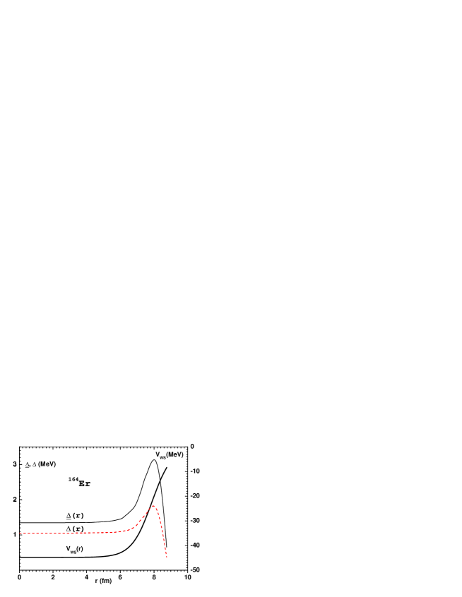
Figure 1: The pair field $\Delta(r,p_{F}(r))$, the value of $\underline{\Delta}=2\tilde{\Delta}=|V_{0}|I^{\kappa\Delta}_{pp}(r,p_{F}(r))$ and the Woods-Saxon potential $V_{WS}(r)$ as the functions of radius $r$.

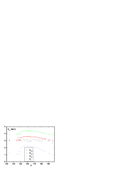
Figure 2: Scissors mode energies as a function of the mass number $A$ for the nuclei listed in Table 1. $E_{new}$: new theory, $E_{old}$: old theory [3], $E_{0}$: theory without pairing.

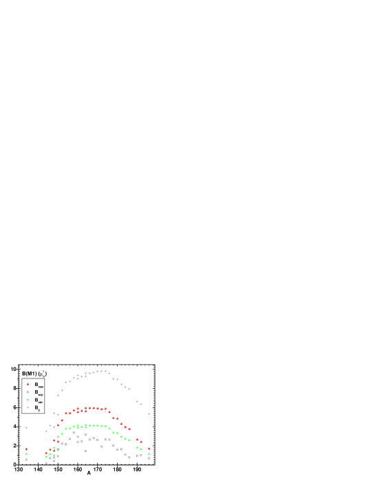
Figure 3: Scissors mode transition probabilities $B(M1)$ as a function of the mass number $A$ for the nuclei listed in Table 1. $B_{new}$: new theory, $B_{old}$: old theory [3], $B_{0}$: theory without pairing.

Another point which should be clarified is the role of the spin-orbit interaction. It is known [2] that the experimentally observed low-lying magnetic dipole strength consists of two separated parts: orbital excitations in the energy interval $\sim$2 – 4 MeV and the spin-flip resonance ranging from 5 to 10 MeV excitation energy. So, for the full description of the scissors mode it would be important to consider also the spin degrees of freedom.

5 Conclusion

In conclusion, we presented a generalization of the method of Wigner function moments which allowed us to include pair correlations without violating the continuity equation. The method was exemplified by the calculation of isovector and isoscalar giant resonances and low-lying excitations in the harmonic oscillator model with quadrupole-quadrupole residual interaction.

The analytical formulae, derived in a slightly simplified model (approximation (21)), reproduce very well the experimentally observed deformation dependence of the energy and $B(M1)$ factor of the scissors mode. We performed calculations for most of the nuclei where this mode has been observed, and our results are in reasonable quantitative agreement with the experimental data, the pair correlations being extremely important.

The joint action of pairing and quantum corrections lead to the appearance of a low-lying isoscalar excitation. The low-lying isoscalar, as well as isovector, modes are very sensitive to the parameters of the interaction and to all details of the ground-state input. Their study on the basis of the full (8 variables) set of dynamical equations (18), with normal and anomalous densities calculated within a microscopic approach, are in progress.

Appendix A

Let us consider integrals containing $\delta\kappa$ and $\delta\Delta$.

The relevant term of the first equation in (12) with $W=p_{x}p_{z}$ reads

$$S=2\int\!d({\bf p},{\bf r})\,p_{x}p_{z}(\Delta^{0}\delta\kappa_{-}-\kappa^{0}\delta\Delta_{-}).$$ (42)

Substituting $\Delta$ and $\delta\Delta$ according to the expressions (9) and (13), one gets

$$S=-\int\!d^{3}r\int\!\frac{2d^{3}p}{(2\pi\hbar)^{3}}\int\!\frac{2d^{3}p^{\prime}}{(2\pi\hbar)^{3}}p_{x}p_{z}v(|{\bf p}-{\bf p}^{\prime}|)[\kappa^{0}({\bf r},{\bf p}^{\prime})\delta\kappa_{-}({\bf r},{\bf p},t)-\kappa^{0}({\bf r},{\bf p})\delta\kappa_{-}({\bf r},{\bf p}^{\prime},t)].$$ (43)

Changing in the second part of the integral the variables $p\leftrightarrow p^{\prime}$, one finds

$$S=-\int\!d^{3}r\int\!\frac{2d^{3}p}{(2\pi\hbar)^{3}}\int\!\frac{2d^{3}p^{\prime}}{(2\pi\hbar)^{3}}v(|{\bf p}-{\bf p}^{\prime}|)\kappa^{0}({\bf r},{\bf p}^{\prime})[p_{x}p_{z}-p^{\prime}_{x}p^{\prime}_{z}]\delta\kappa_{-}({\bf r},{\bf p},t).$$ (44)

Let us analyze in detail the integral over ${\bf p}^{\prime}$

$$\int_{p^{\prime}} = \int\!\frac{2d^{3}p^{\prime}}{(2\pi\hbar)^{3}}v(|{\bf p}-{\bf p}^{\prime}|)\kappa^{0}({\bf r},{\bf p}^{\prime})[p_{x}p_{z}-p^{\prime}_{x}p^{\prime}_{z}]$$ (45)

$$= p_{x}p_{z}\int\!\frac{2d^{3}p^{\prime}}{(2\pi\hbar)^{3}}v(|{\bf p}-{\bf p}^{\prime}|)\kappa^{0}({\bf r},{\bf p}^{\prime})-\int\!\frac{2d^{3}p^{\prime}}{(2\pi\hbar)^{3}}v(|{\bf p}-{\bf p}^{\prime}|)\kappa^{0}({\bf r},{\bf p}^{\prime})p^{\prime}_{x}p^{\prime}_{z}.$$

Now it is necessary to clarify the ${\bf p}$ dependence of $\kappa^{0}$. There are good reasons to assume that it depends only on $|{\bf p}|=p$, i.e., it does not depend on the angles in the momentum space. In fact, according to the semiclassical formula [5]

$$\kappa({\bf r},{\bf p})=\frac{1}{2}\frac{\Delta({\bf r},{\bf p})}{\sqrt{h^{2}({\bf r},{\bf p})+\Delta^{2}({\bf r},{\bf p})}}$$ (46)

the anomalous density can depend on the direction of ${\bf p}$ only via $\Delta({\bf r},{\bf p})$. However, as can be seen from the semiclassical gap equation [5]

$$\Delta({\bf r},{\bf p})=-\frac{1}{2}\int\!\frac{d^{3}p^{\prime}}{(2\pi\hbar)^{3}}v(|{\bf p}-{\bf p}^{\prime}|)\frac{\Delta({\bf r},{\bf p}^{\prime})}{\sqrt{h^{2}({\bf r},{\bf p}^{\prime})+\Delta^{2}({\bf r},{\bf p}^{\prime})}}\,,$$ (47)

there are no reasons to introduce the angular dependence (in momentum space) of $\Delta$ as long as the Fermi surface is spherical. So, it is quite natural to take $\Delta({\bf r},{\bf p})=\Delta({\bf r},p)$ and, as a consequence, $\kappa({\bf r},{\bf p})=\kappa({\bf r},p)$. In this case the integral $\int_{p^{\prime}}$ can be integrated over angles analytically. To this end we expand the pairing force in a standard way [21, 5]:

$$v(|{\bf p}-{\bf p}^{\prime}|)=\sum_{l=0}^{\infty}v_{l}(p,p^{\prime})\sum_{m}Y^{*}_{lm}(\theta,\phi)Y_{lm}(\theta^{\prime},\phi^{\prime}).$$ (48)

Having in mind that $p_{x}p_{z}=\sqrt{\frac{15}{2\pi}}p^{2}(Y_{2-1}-Y_{21})$ we find

$$\int_{p^{\prime}}=2p_{x}p_{z}\int\!\frac{p^{\prime 2}dp^{\prime}}{(2\pi\hbar)^{3}}\kappa^{0}({\bf r},p^{\prime})v_{0}(p,p^{\prime})-2\sqrt{\frac{15}{2\pi}}[Y_{2-1}(\theta,\phi)-Y_{21}(\theta,\phi)]\int\!\frac{p^{\prime 4}dp^{\prime}}{(2\pi\hbar)^{3}}\kappa^{0}({\bf r},p^{\prime})v_{2}(p,p^{\prime}).$$ (49)

If we use a Gaussian as pairing interaction [5]:

$$v(|{\bf p}-{\bf p}^{\prime}|)=\beta e^{-\alpha|{\bf p}-{\bf p}^{\prime}|^{2}}\,,$$ (50)

with $\beta=-|V_{0}|(r_{p}\sqrt{\pi})^{3}$ and $\alpha=r_{p}^{2}/4\hbar^{2}$, the expansion coefficients of the force read [21]:

$$v_{l}(p,p^{\prime})=4\pi\beta e^{-\alpha(p^{2}+p^{\prime 2})}i^{l}j_{l}(-ix),$$ (51)

where $j_{l}(-ix)$ is the spherical Bessel function and $x=2\alpha pp^{\prime}$. We need the first three coefficients

$$v_{0}(p,p^{\prime})=4\pi\beta e^{-\alpha(p^{2}+p^{\prime 2})}\phi_{0}(x),\quad\phi_{0}(x)=\frac{1}{x}sh(x)=(1+\frac{x^{2}}{6}+\dots),$$ (52)

$$v_{1}(p,p^{\prime})=4\pi\beta e^{-\alpha(p^{2}+p^{\prime 2})}x\phi_{1}(x),\quad\phi_{1}(x)=\frac{1}{x^{2}}[ch(x)-\frac{1}{x}sh(x)]=\frac{1}{3}(1+\frac{x^{2}}{10}+\dots),$$ (53)

$$v_{2}(p,p^{\prime})=4\pi\beta e^{-\alpha(p^{2}+p^{\prime 2})}x^{2}\phi_{2}(x),\quad\phi_{2}(x)=\frac{1}{x^{3}}[(1+\frac{3}{x^{2}})sh(x)-\frac{3}{x}ch(x)]=\frac{1}{15}(1+\frac{x^{2}}{14}+\dots).$$ (54)

With the help of these expressions one finds

$$\int_{p^{\prime}}=-p_{x}p_{z}|V_{0}|I^{\kappa\Delta}_{pp}({\bf r},p),$$ (55)

where

$$I^{\kappa\Delta}_{pp}({\bf r},p)=\frac{r_{p}^{3}}{\sqrt{\pi}\hbar^{3}}e^{-\alpha p^{2}}\int\!\kappa^{0}({\bf r},p^{\prime})\left[\phi_{0}(2\alpha pp^{\prime})-4\alpha^{2}p^{\prime 4}\phi_{2}(2\alpha pp^{\prime})\right]e^{-\alpha p^{\prime 2}}p^{\prime 2}dp^{\prime}.$$ (56)

Substituting (55) into (44) one gets finally

$$S = |V_{0}|\int\!d({\bf p},{\bf r})I^{\kappa\Delta}_{pp}({\bf r},p)p_{x}p_{z}\delta\kappa_{-}({\bf r},{\bf p},t)$$ (57)

$$\simeq |V_{0}|I^{\kappa\Delta}_{pp}(\bar{{\bf r}},p_{F})\int\!d({\bf p},{\bf r})p_{x}p_{z}\delta\kappa_{-}({\bf r},{\bf p},t)=|V_{0}|I^{\kappa\Delta}_{pp}(\bar{{\bf r}},p_{F})\tilde{P}_{-}(t).$$

The third and fourth equations of (12) contain the terms

$$T_{\pm}^{W}=\int\!d({\bf p},{\bf r})\,W(1-f_{+}^{0})\delta\Delta_{\pm}.$$ (58)

As above, we assume that $\Delta$ does not depend on the direction of ${\bf p}$. On the basis of the semiclassical formula

$$1-f_{+}^{0}({\bf r},{\bf p})=\frac{h^{0}({\bf r},{\bf p})}{\sqrt{h^{2}({\bf r},{\bf p})+\Delta^{2}({\bf r},{\bf p})}}$$ (59)

we can assume $f_{+}^{0}({\bf r},{\bf p})=f_{+}^{0}({\bf r},p)$, in agreement with the assumption of a spherical Fermi surface. Calculating (58) with $W=xz$, $p_{x}p_{z}$, $\hat{L}$ and $\hat{I}_{y}$ we obtain

$$T_{\pm}^{xz}=|V_{0}|I^{f\Delta}_{xz}(\bar{\bf r},p_{F})\tilde{Q}_{\pm}(t),\quad T_{\pm}^{p_{x}p_{z}}=|V_{0}|I^{f\Delta}_{pp}(\bar{\bf r},p_{F})\tilde{P}_{\pm}(t),$$ (60)

$$T_{\pm}^{L}=|V_{0}|I^{f\Delta}_{xp}(\bar{\bf r},p_{F})\tilde{L}_{\pm}(t),\quad T_{\pm}^{I}=|V_{0}|I^{f\Delta}_{xp}(\bar{\bf r},p_{F})\tilde{I}_{\pm}(t),$$ (61)

where

$$I^{f\Delta}_{xz}({\bf r},p)=\frac{r_{p}^{3}}{2\sqrt{\pi}\hbar^{3}}e^{-\alpha p^{2}}\int\![1-f_{+}^{0}({\bf r},p^{\prime})]\phi_{0}(2\alpha pp^{\prime})e^{-\alpha p^{\prime 2}}p^{\prime 2}dp^{\prime},$$ (62)

$$I^{f\Delta}_{xp}({\bf r},p)=\frac{r_{p}^{5}}{4\sqrt{\pi}\hbar^{5}}e^{-\alpha p^{2}}\int\![1-f_{+}^{0}({\bf r},p^{\prime})]\phi_{1}(2\alpha pp^{\prime})e^{-\alpha p^{\prime 2}}p^{\prime 4}dp^{\prime}.$$ (63)

$$I^{f\Delta}_{pp}({\bf r},p)=\frac{r_{p}^{7}}{8\sqrt{\pi}\hbar^{7}}e^{-\alpha p^{2}}\int\![1-f_{+}^{0}({\bf r},p^{\prime})]\phi_{2}(2\alpha pp^{\prime})e^{-\alpha p^{\prime 2}}p^{\prime 6}dp^{\prime},$$ (64)

The second and third equations of (12) contain the terms

$$K^{W}=2\int\!d({\bf p},{\bf r})\,(\{W,\Delta^{0}\}\delta\kappa_{+}-\{W,\kappa^{0}\}\delta\Delta_{+})$$ (65)

and

$$G^{W}=\int\!d({\bf p},{\bf r})\,\{W,\Delta_{+}^{0}\}\delta f_{-},$$ (66)

which require the knowledge of derivatives of $\Delta^{0}({\bf r},{\bf p})$. They are found with the help of formula (9). The derivative with respect to ${\bf p}$ reads:

$$\frac{\partial\Delta^{0}}{\partial p_{i}}=-\frac{|V_{0}|}{2\hbar^{2}}I_{\partial p}({\bf r},p)p_{i},$$ (67)

where

$$I_{\partial p}({\bf r},p)=\frac{r_{p}^{5}}{2\sqrt{\pi}\hbar^{3}}e^{-\alpha p^{2}}\int\!\kappa^{0}({\bf r},p^{\prime})\left[\phi_{0}(2\alpha pp^{\prime})-2\alpha p^{\prime 2}\phi_{1}(2\alpha pp^{\prime})\right]e^{-\alpha p^{\prime 2}}p^{\prime 2}dp^{\prime}.$$ (68)

To calculate the derivative with respect to ${\bf r}$, we approximate $\kappa^{0}({\bf r},p)$ by formula (46). As a result, we obtain an integral equation for $\partial\Delta^{0}({\bf r},p)/\partial x_{i}$, with a kernel which is strongly peaked at $p^{\prime}=p_{F}$, which allows us to simplify the equation by replacing $\partial\Delta^{0}({\bf r},p^{\prime})/\partial x_{i}$ under the integral by $\partial\Delta^{0}({\bf r},p_{F})/\partial x_{i}$. Finally we have

$$\frac{\partial\Delta^{0}({\bf r},p)}{\partial x_{i}}=\beta({\bf r},p,p_{F})m\omega_{i}^{2}x_{i},$$ (69)

where

$$\beta({\bf r},p,p_{F})=\int\!\frac{p^{\prime 2}dp^{\prime}}{(2\pi\hbar)^{3}}\left[v_{0}(p,p^{\prime})-v_{0}(p_{F},p^{\prime})\frac{\gamma({\bf r},p)}{1+\gamma({\bf r},p_{F})}\right]\frac{h({\bf r},p^{\prime})\Delta({\bf r},p^{\prime})}{2[h^{2}({\bf r},p^{\prime})+\Delta^{2}({\bf r},p^{\prime})]^{3/2}}$$ (70)

and

$$\gamma({\bf r},p)=\int\!\frac{p^{\prime 2}dp^{\prime}}{(2\pi\hbar)^{3}}v_{0}(p,p^{\prime})\frac{h^{2}({\bf r},p^{\prime})}{2[h^{2}({\bf r},p^{\prime})+\Delta^{2}({\bf r},p^{\prime})]^{3/2}}.$$ (71)

Calculating now (66) with $W=xz$, we find

$$G^{xz}=2\int\!d({\bf p},{\bf r})\,(z\frac{\partial\Delta^{0}}{\partial p_{x}}+x\frac{\partial\Delta^{0}}{\partial p_{z}})\delta f_{-}({\bf r},{\bf p},t)=-\frac{|V_{0}|}{\hbar^{2}}I_{\partial p}(\bar{{\bf r}},p_{F})L_{-}(t).$$ (72)

The calculation of (66) with $W=p_{x}p_{z}$ gives

$$G^{pp}=-2\int\!d({\bf p},{\bf r})\,(p_{z}\frac{\partial\Delta^{0}}{\partial x}+p_{x}\frac{\partial\Delta^{0}}{\partial z})\delta f_{-}({\bf r},{\bf p},t)=|V_{0}|I_{\partial r}(\bar{{\bf r}},p_{F})[\omega_{+}^{2}L_{-}(t)-\omega_{-}^{2}I_{-}(t)],$$ (73)

where

$$I_{\partial r}({\bf r},p)=\frac{mr_{p}^{3}}{4\sqrt{\pi}\hbar^{3}}e^{-\alpha p^{2}}\int\!\phi_{0}(2\alpha pp^{\prime})\frac{h({\bf r},p^{\prime})\Delta({\bf r},p^{\prime})-h^{2}({\bf r},p^{\prime})\beta({\bf r},p^{\prime},p_{f})}{[h^{2}({\bf r},p^{\prime})+\Delta^{2}({\bf r},p^{\prime})]^{3/2}}e^{-\alpha p^{\prime 2}}p^{\prime 2}dp^{\prime}.$$ (74)

Calculating (65) with the weight $xp_{z}$, one gets

$$K^{xp_{z}}=-\frac{|V_{0}|}{\hbar^{2}}I^{\{\kappa\Delta\}}_{xp}(\bar{\bf r},p_{F})\tilde{P}_{+}(t),$$ (75)

with

$$I^{\{\kappa\Delta\}}_{xp}({\bf r},p)=\frac{r_{p}^{5}}{2\sqrt{\pi}\hbar^{3}}e^{-\alpha p^{2}}\int\!\kappa^{0}({\bf r},p^{\prime})[\phi_{0}(x)-4\alpha p^{\prime 2}\phi_{1}(x)+4\alpha^{2}p^{\prime 4}\phi_{2}(x)]e^{-\alpha p^{\prime 2}}p^{\prime 2}dp^{\prime},$$ (76)

where $x=2\alpha pp^{\prime}$. It is evident that $K^{xp_{z}}=K^{zp_{x}}$. As a result

$$K^{L}=-2\frac{|V_{0}|}{\hbar^{2}}I^{\{\kappa\Delta\}}_{xp}(\bar{\bf r},p_{F})\tilde{P}_{+}(t),\quad K^{I}=0.$$ (77)

Appendix B

The necessary Poisson brackets are

$$\{xz,h_{0}^{\tau}\}=\frac{1}{m}\hat{L},\quad\{p_{x}p_{z},h_{0}^{\tau}\}=-m(\omega_{z}^{\tau 2}zp_{x}+\omega_{x}^{\tau 2}xp_{z})=-\frac{m}{2}[(\omega_{z}^{\tau 2}+\omega_{x}^{\tau 2})\hat{L}-(\omega_{x}^{\tau 2}-\omega_{z}^{\tau 2})\hat{I}_{y}],$$ (78)

$$\{\hat{L},h_{0}^{\tau}\}=\frac{2}{m}p_{x}p_{z}-m(\omega_{x}^{\tau 2}+\omega_{z}^{\tau 2})xz,\quad\{\hat{I}_{y},h_{0}^{\tau}\}=m(\omega_{z}^{\tau 2}-\omega_{x}^{\tau 2})xz,\quad\{xz,h_{1}^{\tau}\}=0,\quad$$ (79)

$$\{p_{x}p_{z},h_{1}^{\tau}\}=2\delta B_{20}^{\tau}(t)(xp_{z}-2zp_{x})-6[\beta_{11}^{\tau}(t)-\beta_{22}^{\tau}(t)]xp_{z}$$

$$-12[\beta_{13}^{\tau}(t)(zp_{z}+xp_{x})+\beta_{12}^{\tau}(t)yp_{z}+\beta_{23}^{\tau}(t)yp_{x}],$$ (80)

$$\{\hat{L},h_{1}^{\tau}\}=-2\delta B_{20}^{\tau}(t)xz-12[\beta_{13}^{\tau}(t)(z^{2}+x^{2})+\beta_{12}^{\tau}(t)yz+\beta_{23}^{\tau}(t)yx]-6[\beta_{11}^{\tau}(t)-\beta_{22}^{\tau}(t)]xz,$$ (81)

$$\{\hat{I}_{y},h_{1}^{\tau}\}=6\delta B_{20}^{\tau}(t)xz+12[\beta_{23}^{\tau}(t)yx-\beta_{12}^{\tau}(t)yz-\beta_{13}^{\tau}(t)(z^{2}-x^{2})]-6[\beta_{11}^{\tau}(t)-\beta_{22}^{\tau}(t)]xz,$$ (82)

$$\{\{W,h_{0}^{\tau}\}\}=0,\;\{\{xz,h_{1}^{\tau}\}\}=0,\;\{\{p_{x}p_{z},h_{1}^{\tau}\}\}=24\beta_{13}^{\tau}(t),\;\{\{\hat{L},h_{1}^{\tau}\}\}=0,\;\{\{\hat{I}_{y},h_{1}^{\tau}\}\}=0.$$ (83)

Here

$$\beta_{ij}^{\rm n}=\kappa J_{ij}^{\rm n}+\bar{\kappa}J_{ij}^{\rm p},\quad\beta_{ij}^{\rm p}=\kappa J_{ij}^{\rm p}+\bar{\kappa}J_{ij}^{\rm n},$$ (84)

$$J_{ij}^{\tau}(t)=\int\!d({\bf p},{\bf r})x_{i}x_{j}\delta f^{\tau}({\bf r},{\bf p},t),\quad J_{13}^{\tau}(t)=\frac{1}{2}Q_{+}^{\tau}(t),\quad\delta B_{20}^{\tau}(t)=2\beta_{33}^{\tau}(t)-\beta_{11}^{\tau}(t)-\beta_{22}^{\tau}(t).$$ (85)

Using the definition [10] $Q_{20}=\frac{4}{3}Q_{00}\delta$ and the formula $q_{20}=2z^{2}-x^{2}-y^{2}$, one finds from (16)

$$\omega_{x}^{\tau 2}=\omega^{2}(1-\frac{2}{m\omega^{2}}B_{20}^{\tau}),\quad\omega_{x}^{\tau 2}=\omega^{2}(1-\frac{2}{m\omega^{2}}B_{20}^{\tau}).$$ (86)

These oscillator frequencies depend on the strength constants $\kappa_{\rm nn}$ and $\kappa_{\rm np}$. In the isoscalar case the constant $\kappa_{0}=\frac{1}{2}(\kappa_{\rm nn}+\kappa_{\rm np})$ is fixed by the self-consistency condition [10] $\omega_{x}^{2}\langle x^{2}\rangle=\omega_{y}^{2}\langle y^{2}\rangle=\omega_{z}^{2}\langle z^{2}\rangle$, which allows one to find for $\kappa_{0}$ and the oscillator frequencies of the isoscalar field the following expressions [20]:

$$\kappa_{0}=-\frac{m\bar{\omega}^{2}}{4Q_{00}},\quad\omega_{x}^{2}=\frac{1}{2}(\omega_{x}^{\rm n2}+\omega_{x}^{\rm p2})=\bar{\omega}^{2}(1+\frac{4}{3}\delta),\quad\omega_{z}^{2}=\frac{1}{2}(\omega_{z}^{\rm n2}+\omega_{z}^{\rm p2})=\bar{\omega}^{2}(1-\frac{2}{3}\delta),$$ (87)

where $\bar{\omega}^{2}=\omega^{2}/(1+\frac{2}{3}\delta)=\omega_{0}^{2}/[(1+\frac{4}{3}\delta)^{\frac{2}{3}}(1-\frac{2}{3}\delta)^{\frac{1}{3}}],\,$ and $\hbar\omega_{0}=41/A^{1/3}$MeV.

References

• [1] E. B. Balbutsev and P. Schuck, Nucl. Phys. A 720 293 (2003);
E. B. Balbutsev and P. Schuck, Nucl. Phys. A 728 471 (2003).
• [2] D. Zawischa, J. Phys. G: Nucl. Part. Phys. 24 683 (1998).
• [3] E. B. Balbutsev, L. A. Malov, P. Schuck, M. Urban, X. Viñas, Physics of Atomic Nuclei 71, 1012 (2008); arXiv:nucl-th/0701039 v1.
• [4] V. G. Soloviev, Theory of Complex Nuclei (Nauka, Moscow, 1971; Oxford, Pergamon Press, 1976).
• [5] P. Ring and P. Schuck, The Nuclear Many-Body Problem (Springer, Berlin, 1980).
• [6] S. Chandrasekhar, Ellipsoidal Figures of Equilibrium (Yale University Press, New Haven, Conn., 1969).
• [7] E. B. Balbutsev, Sov. J. Part. Nucl. 22 159 (1991).
• [8] E. B. Balbutsev and P. Schuck, Nucl. Phys. A 652 221 (1999).
• [9] M. Urban, Phys. Rev. A 75 053607 (2007).
• [10] A. Bohr and B. Mottelson, Nuclear Structure (Benjamin, New York, 1975), Vol. 2.
• [11] M. Matsuo, Y. Serizawa and K. Mizuyama, arXiv:nucl-th/0608048 v1.
• [12] N. Lo Iudice, La Rivista del Nuovo Cimento 23 N9 (2000).
• [13] I. Hamamoto, C. Magnusson, Phys. Lett. B 260 6 (1991).
• [14] E. Garrido et al., Phys. Rev. C 44 R1250 (1991).
• [15] I. Hamamoto and W. Nazarewicz, Phys. Lett. B 297 25 (1992).
• [16] V. G. Soloviev, A. V. Sushkov, N. Yu. Shirikova and N. Lo Iudice, Nucl. Phys. A 600 155 (1996),
V. G. Soloviev, A. V. Sushkov, N. Yu. Shirikova, Phys. Rev. C 53 1022 (1996).
• [17] M. Macfarlane, J. Speth and D. Zawischa, Nucl. Phys. A 606 41 (1996).
• [18] R. R. Hilton et al., in Proceedings of 1st International Spring Seminar on Nuclear Physics “Microscopic Approaches to Nucler Structure”, Sorrento, 1986, Ed. by A. Covello (Bologna, Physical Society, 1986).
• [19] N. Pietralla et al., Phys. Rev. C 58 184(1998).
• [20] E. B. Balbutsev and P. Schuck, Physics of Atomic Nuclei 69 1985 (2006).
• [21] D. A. Varshalovitch, A. N. Moskalev, and V. K. Khersonski, Quantum Theory of Angular Momentum, Nauka, Leningrad, 1975.