Casimir densities for wedge-shaped boundaries

Abstract

The vacuum expectation values of the field squared and the energy-momentum tensor are investigated for a scalar field with Dirichlet boundary conditions and for the electromagnetic field inside a wedge with a coaxial cylindrical boundary. In the case of the electromagnetic field perfectly conducting boundary conditions are assumed on the bounding surfaces. By using the Abel-Plana-type formula for the series over the zeros of the Bessel function, the vacuum expectation values are presented in the form of the sum of two terms. The first one corresponds to the geometry without a cylindrical boundary and the second one is induced by the presence of the cylindrical shell. The additional vacuum forces acting on the wedge sides due the presence of the cylindrical boundary are evaluated and it is shown that these forces are attractive for both scalar and electromagnetic fields.

PACS numbers: 11.10.Kk, 03.70.+k

1 Introduction

The Casimir effect has important implications on all scales, from cosmological to subnuclear, and has become in recent decades an increasingly popular topic in quantum field theory. Since the original work by Casimir [1] many theoretical and experimental works have been done on this problem (see, e.g., [2, 3] and references therein). In particular, a great deal of attention received the investigations of quantum effects for cylindrical boundaries. In addition to traditional problems of quantum electrodynamics under the presence of material boundaries, the Casimir effect for cylindrical geometries can also be important to the flux tube models of confinement [4] and for determining the structure of the vacuum state in interacting field theories [5]. The calculation of the vacuum energy of electromagnetic field with boundary conditions defined on a cylinder turned out to be technically a more involved problem than the analogous one for a sphere. First the Casimir energy of an infinite perfectly conducting cylindrical shell has been calculated in Ref. [6] by introducing ultraviolet cutoff and later the corresponding result was derived by zeta function technique [7] (for a recent discussion of the Casimir energy and self-stresses in the more general case of a dielectric-diamagnetic cylinder see [8] and references therein). The local characteristics of the corresponding electromagnetic vacuum such as energy density and vacuum stresses are considered in [9] for the interior and exterior regions of a conducting cylindrical shell, and in [10] for the region between two coaxial shells (see also [11]). The vacuum forces acting on the boundaries in the geometry of two cylinders are also considered in Refs. [12]. The scalar Casimir densities for a single and two coaxial cylindrical shells with Robin boundary conditions are investigated in Refs. [13, 14]. Less symmetric configuration of two eccentric perfectly conducting cylinders is considered in [12]. Vacuum energy for a perfectly conducting cylinder of elliptical section is evaluated in Ref. [15] by the mode summation method, using the ellipticity as a perturbation parameter. The Casimir forces acting on two parallel plates inside a conducting cylindrical shell are investigated in Ref. [16]. The Casimir effect in more complicated geometries with cylindrical boundaries is considered in [17].

Aside from their own theoretical and experimental interest, the problems with this type of boundaries are useful for testing the validity of various approximations used to deal with more complicated geometries. From this point of view the wedge with a coaxial cylindrical boundary is an interesting system, since the geometry is nontrivial and it includes two dynamical parameters, radius of the cylindrical shell and opening angle of the wedge. This geometry is also interesting from the point of view of general analysis for surface divergences in the expectation values of local physical observables for boundaries with discontinuities. The nonsmoothness of the boundary generates additional contributions to the heat kernel coefficients (see, for instance, the discussion in [18] and references therein). In the present paper we review the results of the investigations for the vacuum expectation values of the field squared and the energy-momentum tensor for the scalar and electromagnetic fields in the geometry of a wedge with a coaxial cylindrical boundary. In addition to describing the physical structure of the quantum field at a given point, the energy-momentum tensor acts as the source of gravity in the Einstein equations. It therefore plays an important role in modelling a self-consistent dynamics involving the gravitational field. Some most relevant investigations to the present paper are contained in Refs. [2, 19, 20, 21, 22, 23, 24], where the geometry of a wedge without a cylindrical boundary is considered for a conformally coupled scalar and electromagnetic fields in a four dimensional spacetime. The Casimir effect in open geometries with edges is investigated in [25]. The total Casimir energy of a semi-circular infinite cylindrical shell with perfectly conducting walls is considered in [26] by using the zeta function technique. The Casimir energy for the wedge-arc geometry in two dimensions is discussed in [27]. For a scalar field with an arbitrary curvature coupling parameter the Wightman function, the vacuum expectation values of the field squared and the energy-momentum tensor in the geometry of a wedge with an arbitrary opening angle and with a cylindrical boundary are evaluated in [28, 29]. Note that, unlike the case of conformally coupled fields, for a general coupling the vacuum energy-momentum tensor is angle-dependent and diverges on the wedge sides. The corresponding problem for the electromagnetic field, assuming that all boundaries are perfectly conducting, is investigated in [30]. The scalar Casimir densities in the geometry of a wedge with two cylindrical boundaries are discussed in [31]. The closely related problem of the vacuum densities induced by a cylindrical boundary in the geometry of a cosmic string is investigated in Refs. [32] for scalar, electromagnetic and fermionic fields.

We have organized the paper as follows. The next section is devoted to the evaluation of the Wightman function for a scalar field with a general curvature coupling inside a wedge with a cylindrical boundary. By using the formula for the Wightman function, in section 3 we evaluate the vacuum expectation values of the field squared and the energy-momentum tensor inside a wedge without a cylindrical boundary. The vacuum densities for a wedge with the cylindrical shell are considered in section 4. Formulae for the shell contributions are derived and the corresponding surface divergences are investigated. The vacuum expectation values of the electric and magnetic field squared inside a wedge with a cylindrical boundary are investigated in section 5, assuming that all boundaries are perfectly conducting. The corresponding expectation values for the electromagnetic energy-momentum tensor are considered in section 6. The results are summarized in section 7.

2 Wightman function for a scalar field

Consider a free scalar field $\varphi(x)$ inside a wedge with the opening angle $\phi_{0}$ and with a cylindrical boundary of radius $a$ (see figure 1). We will use cylindrical coordinates $(x^{1},x^{2},\ldots,x^{D})=(r,\phi,z_{1},\ldots,z_{N})$, $N=D-2$, where $D$ is the number of spatial dimensions. The field equation has the form

$$\left(\nabla^{i}\nabla_{i}+m^{2}+\xi R\right)\varphi(x)=0,$$ (1)

where $R$ is the scalar curvature for the background spacetime and $\xi$ is the curvature coupling parameter. The special cases $\xi=0$ and $\xi=\xi_{c}=(D-1)/4D$ correspond to minimally and conformally coupled scalars respectively.

In this section we evaluate the positive frequency Wightman function $\langle 0|\varphi(x)\varphi(x^{\prime})|0\rangle$ assuming that the field obeys Dirichlet boundary condition on the bounding surfaces:

$$\varphi|_{\phi=0}=\varphi|_{\phi=\phi_{0}}=\varphi|_{r=a}=0.$$ (2)

The vacuum expectation value (VEV) of the energy-momentum tensor is expressed in terms of the Wightman function as

$$\langle 0|T_{ik}(x)|0\rangle=\lim_{x^{\prime}\rightarrow x}\nabla_{i}\nabla_{k}^{\prime}\langle 0|\varphi(x)\varphi(x^{\prime})|0\rangle+\left[\left(\xi-\frac{1}{4}\right)g_{ik}\nabla^{l}\nabla_{l}-\xi\nabla_{i}\nabla_{k}\right]\langle 0|\varphi^{2}(x)|0\rangle.$$ (3)

In addition, the response of a particle detector in an arbitrary state of motion is determined by this function. In (3) we have assumed that the background spacetime is flat and the term with the Ricci tensor is omitted. The Wightman function is presented as the mode sum

$$\langle 0|\varphi(x)\varphi(x^{\prime})|0\rangle=\sum_{\mathbf{\alpha}}\varphi_{\mathbf{\alpha}}(x)\varphi_{\mathbf{\alpha}}^{\ast}(x^{\prime}),$$ (4)

where $\{\varphi_{\mathbf{\alpha}}(x),\varphi_{\mathbf{\alpha}}^{\ast}(x)\}$ is a complete orthonormal set of solutions to the field equation, satisfying the boundary conditions, $\alpha$ is a set of the corresponding quantum numbers.

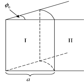
Figure 1: Geometry of a wedge with the opening angle $\phi_{0}$ and cylindrical boundary of radius $a$.

2.1 Interior region

In the region $0\leqslant r\leqslant a$ (region I in figure 1), the eigenfunctions satisfying the boundary conditions (2) on the wedge sides $\phi=0,\phi_{0}$ have the form

$$\varphi_{\alpha}(x) = \beta_{\alpha}J_{qn}(\gamma r)\sin(qn\phi)\exp\left(i\mathbf{kr}_{\parallel}-i\omega t\right),$$ (5)

$$\omega = \sqrt{\gamma^{2}+k_{m}^{2}},\;k_{m}^{2}=|\mathbf{k}|^{2}+m^{2},\quad q=\pi/\phi_{0},$$ (6)

where $\alpha=(n,\gamma,\mathbf{k})$, $-\infty<k_{j}<\infty$, $n=1,2,\cdots$, $\mathbf{k}=(k_{1},\ldots,k_{N})$, $\mathbf{r}_{\parallel}=(z_{1},\ldots,z_{N})$, and $J_{l}(z)$ is the Bessel function. The normalization coefficient $\beta_{\alpha}$ is determined from the standard Klein-Gordon scalar product with the integration over the region inside the wedge and is equal to

$$\beta_{\alpha}^{2}=\frac{2}{(2\pi)^{N}\omega\phi_{0}a^{2}J_{qn}^{\prime 2}(\gamma a)}.$$ (7)

The eigenvalues for the quantum number $\gamma$ are quantized by the boundary condition (2) on the cylindrical surface $r=a$. From this condition it follows that

$$\gamma=\lambda_{n,j}/a,\quad j=1,2,\cdots,$$ (8)

where $\lambda_{n,j}$ are the positive zeros of the Bessel function, $J_{qn}(\lambda_{n,j})=0$, arranged in ascending order, $\lambda_{n,j}<\lambda_{n,j+1}$.

Substituting the eigenfunctions (5) into mode sum formula (4) with the set of quantum numbers $\alpha=(n,j,\mathbf{k})$, for the positive frequency Wightman function one finds

$$\langle 0|\varphi(x)\varphi(x^{\prime})|0\rangle=\int d^{N}\mathbf{k}\,e^{i\mathbf{k}\Delta\mathbf{r}_{\parallel}}\sum_{n=1}^{\infty}\sin(qn\phi)\sin(qn\phi^{\prime})\sum_{j=1}^{\infty}\beta_{\alpha}^{2}J_{qn}(\gamma r)J_{qn}(\gamma r^{\prime})e^{-i\omega\Delta t},$$ (9)

where $\gamma=\lambda_{n,j}/a$, and $\Delta\mathbf{r}_{\parallel}=\mathbf{r}_{\parallel}-\mathbf{r}_{\parallel}^{\prime}$, $\Delta t=t-t^{\prime}$. In order to obtain an alternative form for the Wightman function we apply to the sum over $j$ a variant of the generalized Abel-Plana summation formula [33]

$$\sum_{j=1}^{\infty}\frac{2f(\lambda_{n,j})}{\lambda_{n,j}J_{qn}^{\prime 2}(\lambda_{n,j})} = \int_{0}^{\infty}f(z)dz+\frac{\pi}{4}\mathrm{Res}_{z=0}\left[f(z)\frac{Y_{qn}(z)}{J_{qn}(z)}\right]-$$ (10)

$$+\frac{i}{\pi}\int_{0}^{\infty}dz\,\frac{K_{qn}(z)}{I_{qn}(z)}[e^{-qn\pi i}f(ze^{\pi i/2})-e^{qn\pi i}f(ze^{-\pi i/2})],$$

where $Y_{l}(z)$ is the Neumann function, and $I_{l}(z)$, $K_{l}(z)$ are the modified Bessel functions. The corresponding conditions for the formula (10) to be valid are satisfied if $r+r^{\prime}+|t-t^{\prime}|<2a$. In particular, this is the case in the coincidence limit $t=t^{\prime}$ for the region under consideration, $r,r^{\prime}<a$. Formula (10) allows to present the Wightman function in the form

$$\langle 0|\varphi(x)\varphi(x^{\prime})|0\rangle=\langle 0_{w}|\varphi(x)\varphi(x^{\prime})|0_{w}\rangle+\langle\varphi(x)\varphi(x^{\prime})\rangle_{\mathrm{cyl}},$$ (11)

where

$$\langle 0_{w}|\varphi(x)\varphi(x^{\prime})|0_{w}\rangle = \frac{1}{\phi_{0}}\int\frac{d^{N}\mathbf{k}}{(2\pi)^{N}}e^{i\mathbf{k}\Delta\mathbf{r}_{\parallel}}\int_{0}^{\infty}dz\frac{ze^{-i\Delta t\sqrt{z^{2}+k_{m}^{2}}}}{\sqrt{z^{2}+k_{m}^{2}}}$$ (12)

$$\times\sum_{n=1}^{\infty}\sin(qn\phi)\sin(qn\phi^{\prime})J_{qn}(zr)J_{qn}(zr^{\prime}),$$

and

$$\langle\varphi(x)\varphi(x^{\prime})\rangle_{\mathrm{cyl}} = -\frac{2}{\pi\phi_{0}}\int\frac{d^{N}\mathbf{k}}{(2\pi)^{N}}e^{i\mathbf{k}\Delta\mathbf{r}_{\parallel}}\int_{k_{m}}^{\infty}dz\frac{z\cosh(\Delta t\sqrt{z^{2}-k_{m}^{2}})}{\sqrt{z^{2}-k_{m}^{2}}}$$ (13)

$$\times\sum_{n=1}^{\infty}\sin(qn\phi)\sin(qn\phi^{\prime})I_{qn}(zr)I_{qn}(zr^{\prime})\frac{K_{qn}(za)}{I_{qn}(za)}.$$

In the limit $a\rightarrow\infty$ for fixed $r,r^{\prime}$, the term $\langle\varphi(x)\varphi(x^{\prime})\rangle_{\mathrm{cyl}}$ vanishes whereas the part (12) does not depend on $a$. Hence, the term $\langle 0_{w}|\varphi(x)\varphi(x^{\prime})|0_{w}\rangle$ is the Wightman function for the wedge without a cylindrical boundary with the corresponding vacuum state $|0_{w}\rangle$. Consequently, the term $\langle\varphi(x)\varphi(x^{\prime})\rangle_{\mathrm{cyl}}$ is induced by the presence of the cylindrical boundary. For points away the cylindrical surface this part is finite in the coincidence limit and the renormalization is needed only for the part coming from the term (12).

2.2 Exterior region

In the region outside the cylindrical shell (region II in figure 1): $r>a$, $0\leqslant\phi\leqslant\phi_{0}$, the eigenfunctions satisfying boundary conditions (2) are obtained from (5) by the replacement

$$J_{qn}(\gamma r)\rightarrow g_{qn}(\gamma r,\gamma a)\equiv J_{qn}(\gamma r)Y_{qn}(\gamma a)-J_{qn}(\gamma a)Y_{qn}(\gamma r).$$ (14)

Now the spectrum for the quantum number $\gamma$ is continuous and

$$\beta_{\alpha}^{2}=\frac{(2\pi)^{2-D}\gamma}{\phi_{0}\omega\left[J_{qn}^{2}(\gamma a)+Y_{qn}^{2}(\gamma a)\right]}.$$ (15)

Substituting the corresponding eigenfunctions into the mode sum formula (4), the positive frequency Whightman function in the exterior region is presented in the form

$$\langle 0|\varphi(x)\varphi(x^{\prime})|0\rangle = \frac{1}{\phi_{0}}\int\frac{d^{N}{\mathbf{k}}}{(2\pi)^{N}}e^{i{\mathbf{k}}\Delta\mathbf{r}_{\parallel}}\sum_{n=1}^{\infty}\sin(qn\phi)\sin(qn\phi^{\prime})$$ (16)

$$\times\int_{0}^{\infty}d\gamma\frac{\gamma g_{qn}(\gamma r,\gamma a)g_{qn}(\gamma r^{\prime},\gamma a)}{J_{qn}^{2}(\gamma a)+Y_{qn}^{2}(\gamma a)}\frac{e^{-i\Delta t\sqrt{\gamma^{2}+k_{m}^{2}}}}{\sqrt{\gamma^{2}+k_{m}^{2}}}.$$

To find the part in the Wightman function induced by the presence of the cylindrical shell, we subtract from (16) the corresponding function for the wedge without a cylindrical shell, given by (12). This allows to present the Wightman function in the form (11) with the cylindrical shell induced part

$$\langle\varphi(x)\varphi(x^{\prime})\rangle_{\mathrm{cyl}} = -\frac{2}{\pi\phi_{0}}\int\frac{d^{N}\mathbf{k}}{(2\pi)^{N}}e^{i\mathbf{k}\Delta\mathbf{r}_{\parallel}}\int_{k}^{\infty}dz\frac{z\cosh(\Delta t\sqrt{z^{2}-k^{2}})}{\sqrt{z^{2}-k^{2}}}$$ (17)

$$\times\sum_{n=1}^{\infty}\sin(qn\phi)\sin(qn\phi^{\prime})K_{qn}(zr)K_{qn}(zr^{\prime})\frac{I_{qn}(za)}{K_{qn}(za)}.$$

As we see, the expressions for the Wightman functions in the interior and exterior regions are related by the interchange $I_{qn}\rightleftarrows K_{qn}$ of the modified Bessel functions.

3 VEVs inside a wedge without a cylindrical boundary

In this section we consider the geometry of a wedge without a cylindrical boundary. For integer values of $q$, after the explicit summation over $n$, the Wightman function is presented in the form

$$\langle 0_{w}|\varphi(x)\varphi(x^{\prime})|0_{w}\rangle=\frac{m^{(D-1)/2}}{(2\pi)^{(D+1)/2}}\sum_{j=1}^{2}(-1)^{j+1}\sum_{l=0}^{q-1}\frac{K_{(D-1)/2}(m\sqrt{u_{l}^{(j)2}+|\Delta\mathbf{r}_{\parallel}|^{2}-(\Delta t)^{2}})}{\left[u_{l}^{(j)2}+|\Delta\mathbf{r}_{\parallel}|^{2}-(\Delta t)^{2}\right]^{(D-1)/4}},$$ (18)

where $u_{l}^{(j)}=\{r^{2}+r^{\prime 2}-2rr^{\prime}\cos[2\pi l/q+\phi+(-1)^{j}\phi^{\prime}]\}^{1/2}$. Note that the Wightman function in the Minkowski spacetime coincides with the term $j=1$, $l=0$ in formula (18).

Taking the coincidence limit $x^{\prime}\rightarrow x$, for the difference of the VEVs of the field squared,

$$\langle\varphi^{2}\rangle_{\mathrm{ren}}^{(w)}=\langle 0_{w}|\varphi^{2}(x)|0_{w}\rangle-\langle 0_{M}|\varphi^{2}(x)|0_{M}\rangle,$$ (19)

where $|0_{M}\rangle$ is the amplitude for the vacuum state in the Minkowski spacetime without boundaries, we find

$$\langle\varphi^{2}\rangle_{\mathrm{ren}}^{(w)}=\frac{m^{D-1}}{(2\pi)^{(D+1)/2}}\sum_{j=1}^{2}(-1)^{j+1}\sideset{}{{}^{\prime}}{\sum}_{l=0}^{q-1}\frac{K_{(D-1)/2}(2mr\sin\phi_{l}^{(j)})}{(2mr\sin\phi_{l}^{(j)})^{(D-1)/2}}.$$ (20)

In this formula, the prime means that the term $j=1$, $l=0$ has to be omitted, and we use the notation

$$\phi_{l}^{(j)}=\pi l/q+(1+(-1)^{j})\phi/2.$$ (21)

For a massless field, from (20) we find

$$\langle\varphi^{2}\rangle_{\mathrm{ren}}^{(w)}=\frac{\Gamma\left(\frac{D-1}{2}\right)}{(4\pi)^{\frac{D+1}{2}}r^{D-1}}\sum_{j=1}^{2}\sideset{}{{}^{\prime}}{\sum}_{l=0}^{q-1}\frac{(-1)^{j+1}}{\sin^{D-1}\phi_{l}^{(j)}},$$ (22)

Note that the terms in this formula with $j=2$, $l=0$ and $j=2$, $l=q-1$ are the corresponding VEVs for the geometry of a single plate located at $\phi=0$ and $\phi=\phi_{0}$, respectively. In the case $D=3$ for the renormalized VEV of the field square one finds [20]

$$\langle\varphi^{2}\rangle_{\mathrm{ren}}^{(w)}=\frac{q^{2}-1-3q^{2}\csc^{2}\left(q\phi\right)}{48\pi^{2}r^{2}}.$$ (23)

Near the wedge boundaries $\phi=\phi_{m}$, $m=0,1$ ($\phi_{1}=0$) the main contribution in (22) comes from the terms $j=2$, $l=0$ and $l=q-1$ for $m=0$ and $m=1$ respectively, and the renormalized VEV of the field squared diverges with the leading behaviour $\langle\varphi^{2}\rangle_{\mathrm{ren}}^{(w)}\varpropto|\phi-\phi_{m}|^{1-D}$. The surface divergences in the VEVs of the local physical observables are well known in quantum field theory with boundaries and result from the idealization of the boundaries as perfectly smooth surfaces which are perfect reflectors at all frequencies. These divergences are investigated in detail for various types of fields and general shape of smooth boundary [20, 34]. Near the smooth boundary the leading divergence in the field squared varies as $(D-1)$th power of the distance from the boundary. It seems plausible that such effects as surface roughness, or the microstructure of the boundary on small scales (the atomic nature of matter for the case of the electromagnetic field [35]) can introduce a physical cutoff needed to produce finite values of surface quantities.

Now we turn to the VEVs of the energy-momentum tensor. By making use of formula (3), for the non-zero components one obtains (no summation over $i$)

$$\langle T_{i}^{i}\rangle_{\mathrm{ren}}^{(w)}=-\frac{\Gamma\left(\frac{D+1}{2}\right)}{2^{D+2}\pi^{\frac{D+1}{2}}r^{D+1}}\sum_{j=1}^{2}\sideset{}{{}^{\prime}}{\sum}_{l=0}^{q-1}\frac{(-1)^{j+1}f_{jl}^{(i)}}{\sin^{D+1}\phi_{l}^{(j)}},\;\langle T_{2}^{1}\rangle_{\mathrm{ren}}^{(w)}=\frac{D(\xi_{c}-\xi)\Gamma\left(\frac{D+1}{2}\right)}{2^{D}\pi^{\frac{D+1}{2}}r^{D}}\sum_{l=0}^{q-1}\frac{\cos\phi_{l}^{(2)}}{\sin^{D}\phi_{l}^{(2)}},$$ (24)

where $i=0,1,\ldots,D$, and we use the following notations

$$f_{jl}^{(i)} = 1+\left(4\xi-1\right)\left[(D-1)\delta_{j1}\sin^{2}\phi_{l}^{(j)}+D\delta_{j2}\right],\quad i=0,3,\ldots,D,$$ (25)

$$f_{jl}^{(1)} = f_{jl}^{(0)}-4D(\xi-\xi_{c})\sin^{2}\phi_{l}^{(j)},\;f_{jl}^{(2)}=D\left[4\sin^{2}\phi_{l}^{(j)}\left(\xi-\xi_{c}\delta_{j2}\right)-\delta_{j1}\right].$$ (26)

In the case $\phi_{0}=\pi/2$ and for minimally and conformally coupled scalar fields, it can be checked that from formulae (24), after the transformation from cylindrical coordinates to the cartesian ones, as a special case we obtain the result derived in [36]. For a conformally coupled scalar field $f_{2l}^{(i)}=0$ and from (24) one finds

$$\langle T_{i}^{k}\rangle_{\mathrm{ren}}^{(w)}=-\frac{\Gamma\left(\frac{D+1}{2}\right)}{2^{D+2}\pi^{\frac{D+1}{2}}r^{D+1}}\sum_{l=1}^{q-1}\frac{D-(D-1)\sin^{2}(\pi l/q)}{D\sin^{D+1}(\pi l/q)}\mathrm{diag}(1,1,-D,1,\ldots,1).$$ (27)

In this case the vacuum energy-momentum tensor does not depend on the angular coordinate. For a non-conformally coupled field the VEVs (24) diverge on the boundaries $\phi=\phi_{m}$ and for points away from the edge $r=0$, these divergences are the same as those for the geometry of a single plate.

In the most important case $D=3$, for the components of the renormalized energy-momentum tensor we find

$$\langle T_{0}^{0}\rangle_{\mathrm{ren}}^{(w)} = \langle T_{3}^{3}\rangle_{\mathrm{ren}}^{(w)}=\frac{1}{32\pi^{2}r^{4}}\left\{\frac{1-q^{4}}{45}+\frac{8}{3}\left(1-q^{2}\right)(\xi-\xi_{c})\right.$$ (28)

$$\left.+12\frac{(\xi-\xi_{c})q^{2}}{\sin^{2}(q\phi)}\left[\frac{q^{2}}{\sin^{2}(q\phi)}-\frac{2}{3}q^{2}+\frac{2}{3}\right]\right\},$$

$$\langle T_{1}^{1}\rangle_{\mathrm{ren}}^{(w)} = \frac{1}{32\pi^{2}r^{4}}\left\{\frac{1-q^{4}}{45}-\frac{4}{3}(1-q^{2})(\xi-\xi_{c})\right.$$ (29)

$$\left.+12\frac{(\xi-\xi_{c})q^{2}}{\sin^{2}\left(q\phi\right)}\left[\frac{q^{2}}{\sin^{2}\left(q\phi\right)}-\frac{2}{3}q^{2}-\frac{1}{3}\right]\right\},$$

$$\langle T_{2}^{1}\rangle_{\mathrm{ren}}^{(w)} = -\frac{3(\xi-\xi_{c})}{8\pi^{2}r^{3}}\frac{q^{3}\cos\left(q\phi\right)}{\sin^{3}\left(q\phi\right)},$$ (30)

$$\langle T_{2}^{2}\rangle_{\mathrm{ren}}^{(w)} = \frac{1}{8\pi^{2}r^{4}}\left[\frac{q^{4}-1}{60}+(\xi-\xi_{c})\left(1-q^{2}+\frac{3q^{2}}{\sin^{2}\left(q\phi\right)}\right)\right].$$ (31)

Though we have derived these formulae for integer values of the parameter $q$, by the analytic continuation they are valid for non-integer values of this parameter as well. For a conformally coupled scalar field we obtain the result previously derived in the literature [19, 20]. The corresponding vacuum forces acting on the wedge sides are determined by the effective pressure $-\langle T_{2}^{2}\rangle_{\mathrm{ren}}^{(w)}$. These forces are attractive for the wedge with $q>1$ and are repulsive for $q<1$.

4 Field squared and the energy-momentum tensor

We now turn to the geometry of a wedge with additional cylindrical boundary of radius $a$. Taking the coincidence limit $x^{\prime}\rightarrow x$ in formula (11) for the Wightman function and integrating over $\mathbf{k}$, the VEV of the field squared is presented as the sum of two terms:

$$\langle 0|\varphi^{2}|0\rangle=\langle 0_{w}|\varphi^{2}|0_{w}\rangle+\langle\varphi^{2}\rangle_{\mathrm{cyl}},$$ (32)

where the part induced by the cylindrical boundary is given by the formula

$$\langle\varphi^{2}\rangle_{\mathrm{cyl}}=-\frac{2^{3-D}\pi^{\frac{1-D}{2}}}{\Gamma\left(\frac{D-1}{2}\right)\phi_{0}}\sum_{n=1}^{\infty}\sin^{2}(qn\phi)\int_{m}^{\infty}dz\,z\left(z^{2}-m^{2}\right)^{\frac{D-3}{2}}\frac{K_{qn}(az)}{I_{qn}(az)}I_{qn}^{2}(rz).$$ (33)

Note that this part vanishes at the wedge sides $\phi=\phi_{m}$, $0\leqslant r<a$. Near the edge $r=0$ the main contribution into $\langle\varphi^{2}\rangle_{\mathrm{cyl}}$ comes from the term $n=1$ and $\langle\varphi^{2}\rangle_{\mathrm{cyl}}$ behaves like $r^{2q}$. The part $\langle\varphi^{2}\rangle_{\mathrm{cyl}}$ diverges on the cylindrical surface $r=a$. Near this surface the main contribution into (33) comes from large values $n$ and for $|\phi-\phi_{m}|\gg 1-r/a$ the leading behavior is the same as that for a cylindrical surface of radius $a$.

Similarly, the VEV of the energy-momentum tensor for the situation when the cylindrical boundary is present is written in the form

$$\langle 0|T_{ik}|0\rangle=\langle 0_{w}|T_{ik}|0_{w}\rangle+\langle T_{ik}\rangle_{\mathrm{cyl}},$$ (34)

where $\langle T_{ik}\rangle_{\mathrm{cyl}}$ is induced by the cylindrical boundary. This term is obtained from the corresponding part in the Wightman function, $\langle\varphi(x)\varphi(x^{\prime})\rangle_{\mathrm{cyl}}$, by using formula (3). For points away from the cylindrical surface this limit gives a finite result. For the corresponding components of the energy-momentum tensor one obtains (no summation over $i$)

$$\langle T_{i}^{i}\rangle_{\mathrm{cyl}} = \frac{(4\pi)^{-\frac{D-1}{2}}}{\Gamma\left(\frac{D-1}{2}\right)\phi_{0}}\sum_{n=1}^{\infty}\int_{m}^{\infty}dz\,z^{3}\left(z^{2}-m^{2}\right)^{\frac{D-3}{2}}\frac{K_{qn}(az)}{I_{qn}(az)}$$ (35)

$$\times\left\{a_{i,qn}^{(+)}[I_{qn}(rz)]-a_{i,qn}^{(-)}[I_{qn}(rz)]\cos(2qn\phi)\right\},$$

$$\langle T_{2}^{1}\rangle_{\mathrm{cyl}} = \frac{2(4\pi)^{-\frac{D-1}{2}}}{\Gamma\left(\frac{D-1}{2}\right)\phi_{0}}\sum_{n=1}^{\infty}qn\sin(2qn\phi)\int_{m}^{\infty}dz\,z^{2}(z^{2}-m^{2})^{\frac{D-3}{2}}\frac{K_{qn}(az)}{I_{qn}(az)}$$ (36)

$$\times I_{qn}(rz)\left[\frac{2\xi}{rz}I_{qn}(rz)+(1-4\xi)I_{qn}^{\prime}(rz)\right],$$

with the notations

$$a_{i,l}^{(\pm)}[g(y)] = (4\xi-1)\left[g^{\prime 2}(y)+\left(1\pm l^{2}/y^{2}\right)g^{2}(y)\right]+2g^{2}(y)\frac{1-m^{2}r^{2}/y^{2}}{D-1},$$

$$a_{1,l}^{(\pm)}[g(y)] = g^{\prime 2}(y)+(4\xi/y)g(y)g^{\prime}(y)-g^{2}(y)\left\{1\pm\left[1-4\xi(1\mp 1)\right]l^{2}/y^{2}\right\},$$ (37)

$$a_{2,l}^{(\pm)}[g(y)] = \left(4\xi-1\right)\left[g^{\prime 2}(y)+g^{2}(y)\right]-(4\xi/y)g(y)g^{\prime}(y)+g^{2}(y)\left(4\xi\pm 1\right)l^{2}/y^{2},$$

for a given function $g(y)$, $i=0,3,\ldots,D$. In accordance with the problem symmetry, the expressions for the diagonal components are invariant under the replacement $\phi\rightarrow\phi_{0}-\phi$, and the off-diagonal component $\langle T_{2}^{1}\rangle_{\mathrm{cyl}}$ changes the sign under this replacement. Note that the latter vanishes on the wedge sides $\phi=\phi_{m}$, $0\leqslant r<a$ and for $\phi=\phi_{0}/2$. On the wedge sides for the diagonal components of the energy-momentum tensor we obtain (no summation over $i$)

$$\langle T_{i}^{i}\rangle_{\mathrm{cyl},\phi=\phi_{m}}=\frac{2^{2-D}\pi^{\frac{5-D}{2}}A_{i}}{\Gamma\left(\frac{D-1}{2}\right)r^{2}\phi_{0}^{3}}\sum_{n=1}^{\infty}n^{2}\int_{m}^{\infty}dz\,z\left(z^{2}-m^{2}\right)^{\frac{D-3}{2}}\frac{K_{qn}(az)}{I_{qn}(az)}I_{qn}^{2}(rz),$$ (38)

where $A_{i}=4\xi-1$, $i=0,1,3,\ldots,D$, $A_{2}=1$. In particular, the additional vacuum effective pressure in the direction perpendicular to the wedge sides, $p_{a}=-\langle T_{2}^{2}\rangle_{\mathrm{cyl},\phi=\phi_{m}}$, does not depend on the curvature coupling parameter and is negative for all values $0<r<a$. This means that the vacuum forces acting on the wedge sides due to the presence of the cylindrical boundary are attractive. The corresponding vacuum stresses in the directions parallel to the wedge sides are isotropic and the energy density is negative for both minimally and conformally coupled scalars.

For $0<r<a$ the cylindrical parts (35) and (36) are finite for all values $0\leqslant\phi\leqslant\phi_{0}$, including the wedge sides. The divergences on these sides are included in the first term on the right-hand side of (34) corresponding to the case without cylindrical boundary. Near the edge $r=0$ the main contribution into the boundary parts comes from the summand with $n=1$ and one has $\langle T_{i}^{i}\rangle_{\mathrm{cyl}}\propto r^{2q-2}$, $\langle T_{2}^{1}\rangle_{\mathrm{cyl}}\propto r^{2q-1}$. The boundary part $\left\langle T_{i}^{k}\right\rangle_{\mathrm{cyl}}$ diverges on the cylindrical surface $r=a$. Expanding over $a-r$, on the wedge sides for the diagonal components one finds

$$\langle T_{i}^{i}\rangle_{\mathrm{cyl},\phi=\phi_{m}}\approx\frac{A_{i}\Gamma\left(\frac{D+1}{2}\right)}{2(4\pi)^{\frac{D+1}{2}}(a-r)^{D+1}},\quad r\rightarrow a,$$ (39)

where the coefficients $A_{i}$ are defined in the paragraph after formula (38). It can be seen that for the off-diagonal component to the leading order one has $\langle T_{2}^{1}\rangle_{a}\varpropto(a-r)^{-D}$. For angles $0<\phi<\phi_{0}$, and for $|\phi-\phi_{m}|\gg 1-r/a$, the leading divergence coincides with the corresponding one for a cylindrical surface of the radius $a$.

Taking the coincidence limit of the arguments, from formula (17) we obtain the VEV of the field squared in the region $r>a$:

$$\langle\varphi^{2}\rangle_{\mathrm{cyl}}=-\frac{2^{3-D}\pi^{\frac{1-D}{2}}}{\Gamma\left(\frac{D-1}{2}\right)\phi_{0}}\sum_{n=1}^{\infty}\sin^{2}(qn\phi)\int_{m}^{\infty}dz\,z\left(z^{2}-m^{2}\right)^{\frac{D-3}{2}}\frac{I_{qn}(az)}{K_{qn}(az)}K_{qn}^{2}(rz).$$ (40)

As for the interior region, the VEV (40) diverges on the cylindrical surface. For large distances from the cylindrical surface, $r\gg a$, and for a massless field the main contribution comes from the $n=1$ term and to the leading order one finds $\langle\varphi^{2}\rangle_{\mathrm{cyl}}\varpropto(a/r)^{D-1+2q}$. For a massive field and for $mr\gg 1$ the part $\langle\varphi^{2}\rangle_{\mathrm{cyl}}$ is exponentially suppressed.

For the part in the vacuum energy-momentum tensor induced by the cylindrical surface in the region $r>a$, from (3), (17), (40) one has the following formulae

$$\langle T_{i}^{i}\rangle_{\mathrm{cyl}} = \frac{(4\pi)^{-\frac{D-1}{2}}}{\Gamma\left(\frac{D-1}{2}\right)\phi_{0}}\sum_{n=1}^{\infty}\int_{m}^{\infty}dz\,z^{3}\left(z^{2}-m^{2}\right)^{\frac{D-3}{2}}\frac{I_{qn}(az)}{K_{qn}(az)}$$ (41)

$$\times\left\{a_{i,qn}^{(+)}[K_{qn}(rz)]-a_{i,qn}^{(-)}[K_{qn}(rz)]\cos(2qn\phi)\right\},$$

$$\langle T_{2}^{1}\rangle_{\mathrm{cyl}} = \frac{2(4\pi)^{-\frac{D-1}{2}}}{\Gamma\left(\frac{D-1}{2}\right)\phi_{0}}\sum_{n=1}^{\infty}qn\sin(2qn\phi)\int_{m}^{\infty}dz\,\,z^{2}(z^{2}-m^{2})^{\frac{D-3}{2}}\frac{I_{qn}(az)}{K_{qn}(az)}$$ (42)

$$\times K_{qn}(rz)\left[\frac{2\xi}{rz}K_{qn}(rz)+(1-4\xi)K_{qn}^{\prime}(rz)\right],$$

with the functions $a_{i,qn}^{(\pm)}[g(y)]$ defined by (37). In the way similar to that used above for the VEV of the field square, it can be seen that at large distances from the cylindrical surface, $r\gg a$, the main contribution comes from the term with $n=1$ and for a massless field the components of the induced energy-momentum tensor behave as $\langle T_{i}^{i}\rangle_{\mathrm{cyl}}\varpropto(a/r)^{D+1+2q}$, $\langle T_{2}^{1}\rangle_{\mathrm{cyl}}\varpropto(a/r)^{D+2q}$. As for the interior region, the vacuum forces acting on the wedge sides due to the presence of the cylindrical shell are attractive and the corresponding energy density is negative for both minimally and conformally coupled scalars.

In the limit $\phi_{0}\rightarrow 0$, $r,a\rightarrow\infty$, assuming that $a-r$ and $a\phi_{0}\equiv b$ are fixed, from the results given above we obtain the vacuum densities for the geometry of two parallel plates separated by a distance $b$, perpendicularly intersected by the third plate. The vacuum expectation values of the energy-momentum tensor for this geometry of boundaries are investigated in [36] for special cases of minimally and conformally coupled massless scalar fields.

5 VEVs for the electromagnetic fields

5.1 Interior region

In this section we consider a wedge with a coaxial cylindrical boundary assuming that all boundaries are perfectly conducting. For this geometry there are two different types of the eigenfunctions corresponding to the transverse magnetic (TM, $\lambda=0$) and transverse electric (TE, $\lambda=1$) waves. In the Coulomb gauge, the vector potentials for these modes are given by the formulae

$$\mathbf{A}_{\alpha}=\beta_{\alpha}\left\{\begin{array}[]{cc}(1/i\omega)\left(\gamma^{2}\mathbf{e}_{3}+ik\nabla_{t}\right)J_{qn}(\gamma r)\sin(qn\phi)\exp\left[i\left(kz-\omega t\right)\right],&\lambda=0\\ -\mathbf{e}_{3}\times\nabla_{t}\left\{J_{qn}(\gamma r)\cos(qn\phi)\exp\left[i\left(kz-\omega t\right)\right]\right\},&\lambda=1\end{array}\right.,$$ (43)

where $\mathbf{e}_{3}$ is the unit vector along the axis of the wedge, $\nabla_{t}$ is the part of the nabla operator transverse to this axis, and $\omega^{2}=\gamma^{2}+k^{2}$. In Eq. (43), $n=1,2,\ldots$ for $\lambda=0$ and $n=0,1,2,\ldots$ for $\lambda=1$. From the normalization condition one finds

$$\beta_{\alpha}^{2}=\frac{4qT_{qn}(\gamma a)}{\pi\omega a\gamma}\delta_{n},\;\delta_{n}=\left\{\begin{array}[]{cc}1/2,&n=0\\ 1,&n\neq 0\end{array}\right.,$$ (44)

where we have introduced the notation $T_{\nu}(x)=x\left[J_{\nu}^{{}^{\prime}2}(x)+(1-\nu^{2}/x^{2})J_{\nu}^{2}(x)\right]^{-1}$. Eigenfunctions (43) satisfy the standard boundary conditions on the wedge sides. From the boundary conditions on the cylindrical shell it follows that the eigenvalues for $\gamma$ are roots of the equation

$$J_{qn}^{(\lambda)}(\gamma a)=0,\quad\lambda=0,1,$$ (45)

where $J_{\nu}^{(0)}(x)=J_{\nu}(x)$ and $J_{\nu}^{(1)}(x)=J_{\nu}^{\prime}(x)$. We will denote the corresponding eigenmodes by $\gamma a=\lambda_{n,j}^{(\lambda)}$, $j=1,2,\ldots$.

First we consider the VEVs of the squares of the electric and magnetic fields inside the shell. Substituting the eigenfunctions (43) into the corresponding mode-sum formula, we find

$$\langle 0|F^{2}|0\rangle=\frac{4q}{\pi a^{3}}\sideset{}{{}^{\prime}}{\sum}_{m=0}^{\infty}\int_{-\infty}^{+\infty}dk\sum_{\lambda=0,1}\sum_{n=1}^{\infty}\frac{\lambda_{n,j}^{(\lambda)3}T_{qm}(\lambda_{n,j}^{(\lambda)})}{\sqrt{\lambda_{n,j}^{(\lambda)2}+k^{2}a^{2}}}g^{(\eta_{F\lambda})}[\Phi_{qn}^{(\lambda)}(\phi),J_{qn}(\lambda_{n,j}^{(\lambda)}r/a)],$$ (46)

where $F=E,B$ with $\eta_{E\lambda}=\lambda$, $\eta_{B\lambda}=1-\lambda$, and the prime in the summation over $n$ means that the term $n=0$ should be halved. In formula (46) we have introduced the notations

$$g^{(0)}[\Phi(\phi),f(x)] = (k^{2}r^{2}/x^{2})\left[\Phi^{2}(\phi)f^{\prime 2}(x)+\Phi^{\prime 2}(\phi)f^{2}(x)/x^{2}\right]+\Phi^{2}(\phi)f^{2}(x),$$

$$g^{(1)}[\Phi(\phi),f(x)] = (1+k^{2}r^{2}/x^{2})\left[\Phi^{2}(\phi)f^{\prime 2}(x)+\Phi^{\prime 2}(\phi)f^{2}(x)/x^{2}\right],$$ (47)

and

$$\Phi_{\nu}^{(0)}(\phi)=\sin(\nu\phi),\;\Phi_{\nu}^{(1)}(\phi)=\cos(\nu\phi).$$ (48)

The expressions (46) corresponding to the electric and magnetic fields are divergent. They may be regularized introducing a cutoff function $\psi_{\mu}(\omega)$ with the cutting parameter $\mu$ which makes the divergent expressions finite and satisfies the condition $\psi_{\mu}(\omega)\rightarrow 1$ for $\mu\rightarrow 0$. After the renormalization the cutoff function is removed by taking the limit $\mu\rightarrow 0$.

In order to further simplify the VEVs, we apply to the series over $n$ the summation formula (10) for the modes with $\lambda=0$ and the similar formula from [33] for the modes with $\lambda=1$. As it can be seen, for points away from the shell the contribution to the VEVs coming from the second integral terms on the right-hand sides of these formulae are finite in the limit $\mu\rightarrow 0$ and, hence, the cutoff function in these terms can be safely removed. As a result the VEVs are written in the form

$$\langle 0|F^{2}|0\rangle=\langle 0_{w}|F^{2}|0_{w}\rangle+\left\langle F^{2}\right\rangle_{\mathrm{cyl}},$$ (49)

where

$$\langle 0_{w}|F^{2}|0_{w}\rangle = \frac{q}{\pi}\sideset{}{{}^{\prime}}{\sum}_{n=0}^{\infty}\int_{-\infty}^{+\infty}dk\int_{0}^{\infty}d\gamma\,\frac{\gamma^{3}\psi_{\mu}(\omega)}{\sqrt{\gamma^{2}+k^{2}}}\left\{\left(1+\frac{2k^{2}}{\gamma^{2}}\right)\left[J_{qn}^{\prime 2}(\gamma r)+\frac{q^{2}n^{2}}{\gamma^{2}r^{2}}J_{qn}^{2}(\gamma r)\right]\right.$$ (50)

$$\left.+J_{qn}^{2}(\gamma r)-(-1)^{\eta_{F1}}\cos(2qn\phi)\left[J_{qn}^{\prime 2}(\gamma r)-\left(1+\frac{q^{2}n^{2}}{\gamma^{2}r^{2}}\right)J_{qn}^{2}(\gamma r)\right]\right\},$$

and

$$\langle F^{2}\rangle_{\mathrm{cyl}}=\frac{2q}{\pi}\sideset{}{{}^{\prime}}{\sum}_{n=0}^{\infty}\sum_{\lambda=0,1}\int_{0}^{\infty}dx\,x^{3}\frac{K_{qn}^{(\lambda)}(xa)}{I_{qn}^{(\lambda)}(xa)}G^{(\eta_{F\lambda})}[\Phi_{qn}^{(\lambda)}(\phi),I_{qn}(xr)].$$ (51)

In formula (51) we have introduced the notations

$$G^{(0)}[\Phi(\phi),f(x)] = \Phi^{2}(\phi)f^{\prime 2}(x)+\Phi^{\prime 2}(\phi)f^{2}(x)/x^{2}+2\Phi^{2}(\phi)f^{2}(x),$$

$$G^{(1)}[\Phi(\phi),f(x)] = -\Phi^{2}(\phi)f^{\prime 2}(x)-\Phi^{\prime 2}(\phi)f^{2}(x)/x^{2}.$$ (52)

The second term on the right-hand side of Eq. (49) vanishes in the limit $a\rightarrow\infty$ and the first one does not depend on $a$. Thus, we can conclude that the term $\langle 0_{w}|F^{2}|0_{w}\rangle$ corresponds to the part in the VEVs when the cylindrical shell is absent.

First, let us concentrate on the part corresponding to the wedge without a cylindrical shell. In (50) the part which does not depend on the angular coordinate $\phi$ is the same as in the corresponding problem of the cosmic string geometry with the angle deficit $2\pi-\phi_{0}$ (see [32]), which we will denote by $\langle 0_{\mathrm{s}}|F^{2}|0_{\mathrm{s}}\rangle$. For this part we have

$$\langle 0_{\mathrm{s}}|F^{2}|0_{\mathrm{s}}\rangle=\langle 0_{\mathrm{M}}|F^{2}|0_{\mathrm{M}}\rangle-\frac{(q^{2}-1)(q^{2}+11)}{180\pi r^{4}},$$ (53)

where $\langle 0_{\mathrm{M}}|F^{2}|0_{\mathrm{M}}\rangle$ is the VEV in the Minkowski spacetime without boundaries and in the last expression we have removed the cutoff. To evaluate the part in (50) which depends on $\phi$, we firstly consider the case when the parameter $q$ is an integer. In this case, the summation over $n$ can be done explicitly and the integrals are evaluated by introducing polar coordinates in the $(k,\gamma)$-plane. As a result, for the renormalised VEVs of the field squared in the geometry of a wedge without a cylindrical boundary we find

$$\langle F^{2}\rangle_{\mathrm{ren}}^{(w)}=-\frac{(q^{2}-1)(q^{2}+11)}{180\pi r^{4}}-\frac{(-1)^{\eta_{F1}}q^{2}}{2\pi r^{4}\sin^{2}(q\phi)}\left[1-q^{2}+\frac{3q^{2}}{2\sin^{2}(q\phi)}\right],$$ (54)

with $\eta_{E1}=1$ and $\eta_{B1}=0$. Though we have derived this formula for integer values of the parameter $q$, by the analytic continuation it is valid for non-integer values of this parameter as well. The expression on the right of formula (54) is invariant under the replacement $\phi\rightarrow\phi_{0}-\phi$ and, as we could expect, the VEVs are symmetric with respect to the half-plane $\phi=\phi_{0}/2$. Formula (54) for $F=E$ was derived in Ref. [22] within the framework of Schwinger’s source theory.

Now, we turn to the investigation of the parts in the VEVs of the field squared induced by the cylindrical boundary and given by formula (51). These parts are symmetric with respect to the half-plane $\phi=\phi_{0}/2$. The expression in the right-hand side of (51) is finite for $0<r<a$ including the points on the wedge sides, and diverges on the shell. To find the leading term in the corresponding asymptotic expansion, we note that near the shell the main contribution comes from large values of $n$. By using the uniform asymptotic expansions of the modified Bessel functions for large values of the order, up to the leading order, for the points $a-r\ll a|\sin\phi|,a|\sin(\phi_{0}-\phi)|$ we find $\langle F^{2}\rangle_{\mathrm{cyl}}\approx-3(-1)^{\eta_{F1}}/[4\pi(a-r)^{4}]$. These surface divergences originate in the unphysical nature of perfect conductor boundary conditions. In reality the expectation values will attain a limiting value on the conductor surface, which will depend on the molecular details of the conductor. From the formulae given above it follows that the main contribution to $\langle F^{2}\rangle_{\mathrm{cyl}}$ are due to the frequencies $\omega\lesssim(a-r)^{-1}$. Hence, we expect that formula (51) is valid for real conductors up to distances $r$ for which $(a-r)^{-1}\ll\omega_{0}$, with $\omega_{0}$ being the characteristic frequency, such that for $\omega>\omega_{0}$ the conditions for perfect conductivity fail.

Near the edge $r=0$, assuming that $r/a\ll 1$, the asymptotic behavior of the part induced in the VEVs of the field squared by the cylindrical shell depends on the parameter $q$. For $q>1+\eta_{F1}$, the dominant contribution comes from the lowest mode $n=0$ and to the leading order one has $\langle F^{2}\rangle_{\mathrm{cyl}}\varpropto r^{2\eta_{F1}}$. In this case the quantity $\langle B^{2}\rangle_{\mathrm{cyl}}$ takes a finite limiting value on the edge $r=0$, whereas $\langle E^{2}\rangle_{\mathrm{cyl}}$ vanishes as $r^{2}$. For $q<1+\eta_{F1}$ the main contribution comes from the mode with $n=1$ and the shell-induced parts diverge on the edge $r=0$ with $\langle F^{2}\rangle_{\mathrm{cyl}}\varpropto r^{2(q-1)}$. In accordance with (54), near the edge $r=0$ the total VEV is dominated by the part coming from the wedge without the cylindrical shell.

5.2 Exterior region

In the exterior region (region II in figure 1), the corresponding eigenfunctions for the vector potential are obtained from formulae (43) by the replacement

$$J_{qn}(\gamma r)\rightarrow g_{qn}^{(\lambda)}(\gamma a,\gamma r)=J_{qn}(\gamma r)Y_{qn}^{(\lambda)}(\gamma a)-Y_{qn}(\gamma r)J_{qn}^{(\lambda)}(\gamma a),$$ (55)

where, as before, $\lambda=0,1$ correspond to the waves of the electric and magnetic types, respectively. The eigenvalues for $\gamma$ are continuous and

$$\beta_{\alpha}^{-2}=(8\pi/q)\delta_{n}\gamma\omega\left[J_{qn}^{(\lambda)2}(\gamma a)+Y_{qn}^{(\lambda)2}(\gamma a)\right].$$ (56)

Substituting the eigenfunctions into the corresponding mode-sum formula, for the VEV of the field squared one finds

$$\langle 0|F^{2}|0\rangle=\frac{2q}{\pi}\sideset{}{{}^{\prime}}{\sum}_{n=0}^{\infty}\int_{-\infty}^{+\infty}dk\int_{0}^{\infty}d\gamma\sum_{\lambda=0,1}\frac{\gamma^{3}}{\sqrt{k^{2}+\gamma^{2}}}\frac{g^{(\eta_{F\lambda})}[\Phi_{qn}^{(\lambda)}(\phi),g_{qn}^{(\lambda)}(\gamma a,\gamma r)]}{J_{qn}^{(\lambda)2}(\gamma a)+Y_{qn}^{(\lambda)2}(\gamma a)},$$ (57)

where the functions $g^{(\eta_{F\lambda})}[\Phi(\phi),f(x)]$ are defined by relations (47) with $f(x)=g_{qn}^{(\lambda)}(\gamma a,x)$. To extract from this VEV the part induced by the cylindrical shell, we subtract from the right-hand side the corresponding expression for the wedge without the cylindrical boundary. As a result, the VEV of the field squared is written in the form (49), where the part induced by the cylindrical shell is given by the formula

$$\langle F^{2}\rangle_{\mathrm{cyl}}=\frac{2q}{\pi}\sideset{}{{}^{\prime}}{\sum}_{n=0}^{\infty}\sum_{\lambda=0,1}\int_{0}^{\infty}dx\,x^{3}\frac{I_{qn}^{(\lambda)}(xa)}{K_{qn}^{(\lambda)}(xa)}G^{(\eta_{F\lambda})}[\Phi_{qn}^{(\lambda)}(\phi),K_{qn}(xr)].$$ (58)

In this formula the functions $G^{(\eta_{F\lambda})}\left[\Phi(\phi),f(x)\right]$ are defined by expressions (52). Comparing this result with formula (51), we see that the expressions for the shell-induced parts in the interior and exterior regions are related by the interchange $I_{qn}\rightleftarrows K_{qn}$.

The VEV (58) diverges on the cylindrical shell with the leading term being the same as that for the interior region. At large distances from the cylindrical shell we introduce a new integration variable $y=xr$ and expand the integrand over $a/r$. For $q>1$ the main contribution comes from the lowest mode $n=0$ and up to the leading order we have

$$\langle E^{2}\rangle_{\mathrm{cyl}}\approx\frac{4q\left(a/r\right)^{2}}{5\pi r^{4}},\;\langle B^{2}\rangle_{\mathrm{cyl}}\approx-\frac{28q\left(a/r\right)^{2}}{15\pi r^{4}}.$$ (59)

For $q<1$ the dominant contribution into the VEVs at large distances is due to the mode $n=1$ with the leading term

$$\langle F^{2}\rangle_{\mathrm{cyl}}\approx-\frac{4q^{2}(q+1)}{\pi r^{4}}\left(\frac{a}{r}\right)^{2q}\left[\frac{\cos(2q\phi)}{2q+3}+(-1)^{\eta_{F1}}\frac{q+1}{2q+1}\right].$$ (60)

For the case $q=1$ the contributions of the modes $n=0$ and $n=1$ are of the same order and the corresponding leading terms are obtained by summing these contributions. The latter are given by the right-hand sides of formulae (59) and (60). As we see, at large distances the part induced by the cylindrical shell is suppressed with respect to the part corresponding to the wedge without the shell by the factor $(a/r)^{2\beta}$ with $\beta=\min(1,q)$.

6 Energy-momentum tensor for the electromagnetic field

Now let us consider the VEV of the energy-momentum tensor in the region inside the cylindrical shell. Substituting the eigenfunctions (43) into the corresponding mode-sum formula, for the non-zero components we obtain (no summation over $i$)

$$\langle 0|T_{i}^{i}|0\rangle = \frac{q}{2\pi^{2}a^{3}}\sideset{}{{}^{\prime}}{\sum}_{n=0}^{\infty}\int_{-\infty}^{+\infty}dk\sum_{\lambda=0,1}\sum_{j=1}^{\infty}\frac{\lambda_{n,j}^{(\lambda)3}T_{qn}(\lambda_{n,j}^{(\lambda)})}{\sqrt{\lambda_{n,j}^{(\lambda)2}+k^{2}a^{2}}}f^{(i)}[\Phi_{qn}^{(\lambda)}(\phi),J_{qn}(\lambda_{n,j}^{(\lambda)}r/a)],$$ (61)

$$\langle 0|T_{2}^{1}|0\rangle = \frac{-q^{2}}{4\pi^{2}a}\frac{\partial}{\partial r}\sideset{}{{}^{\prime}}{\sum}_{n=0}^{\infty}n\sin(2qn\phi)\int_{-\infty}^{+\infty}dk\sum_{\lambda=0,1}(-1)^{\lambda}$$ (62)

$$\times\sum_{j=1}^{\infty}\frac{\lambda_{n,j}^{(\lambda)}T_{qn}(\lambda_{n,j}^{(\lambda)})}{\sqrt{\lambda_{n,j}^{(\lambda)2}+k^{2}a^{2}}}J_{qn}^{2}(\lambda_{n,j}^{(\lambda)}r/a),$$

where $i=0,1,2,3$, and we have introduced the notations

$$f^{(j)}[\Phi(\phi),f(x)] = (-1)^{i}\left(2k^{2}/\gamma^{2}+1\right)\left[\Phi^{2}(\phi)f^{\prime 2}(x)+\Phi^{\prime 2}(\phi)f^{2}(x)/y^{2}\right]+\Phi^{2}(\phi)f^{2}(x),$$

$$f^{(l)}[\Phi(\phi),f(x)] = (-1)^{l}\Phi^{2}(\phi)f^{\prime 2}(x)-\left[\Phi^{2}(\phi)+(-1)^{l}\Phi^{\prime 2}(\phi)/x^{2}\right]f^{2}(x),$$ (63)

with $j=0,3$ and $l=1,2$. As in the case of the field squared, in formulae (61) and (62) we introduce a cutoff function and apply formula (10) for the summation over $n$. This enables us to present the vacuum energy-momentum tensor in the form of the sum

$$\langle 0|T_{i}^{k}|0\rangle=\langle 0_{w}|T_{i}^{k}|0_{w}\rangle+\langle T_{i}^{k}\rangle_{\mathrm{cyl}},$$ (64)

where $\langle 0_{w}|T_{i}^{k}|0_{w}\rangle$ is the part corresponding to the geometry of a wedge without a cylindrical boundary and $\langle T_{i}^{k}\rangle_{\mathrm{cyl}}$ is induced by the cylindrical shell. The latter may be written in the form (no summation over $i$)

$$\langle T_{i}^{i}\rangle_{\mathrm{cyl}} = \frac{q}{2\pi^{2}}\sideset{}{{}^{\prime}}{\sum}_{n=0}^{\infty}\sum_{\lambda=0,1}\int_{0}^{\infty}dxx^{3}\frac{K_{qn}^{(\lambda)}(xa)}{I_{qn}^{(\lambda)}(xa)}F^{(i)}[\Phi_{qn}^{(\lambda)}(\phi),I_{qn}(xr)],$$ (65)

$$\langle T_{2}^{1}\rangle_{\mathrm{cyl}} = \frac{q^{2}}{4\pi^{2}}\frac{\partial}{\partial r}\sideset{}{{}^{\prime}}{\sum}_{n=0}^{\infty}n\sin(2qn\phi)\sum_{\lambda=0,1}(-1)^{\lambda}\int_{0}^{\infty}dxx\frac{K_{qn}^{(\lambda)}(xa)}{I_{qn}^{(\lambda)}(xa)}I_{qn}^{2}(xr),$$ (66)

with the notations

$$F^{(i)}[\Phi(\phi),f(y)] = \Phi^{2}(\phi)f^{2}(y),\;i=0,3,$$

$$F^{(i)}[\Phi(\phi),f(y)] = -(-1)^{i}\Phi^{2}(\phi)f^{\prime 2}(y)-\left[\Phi^{2}(\phi)-(-1)^{i}\Phi^{\prime 2}(\phi)/y^{2}\right]f^{2}(y),\;i=1,2.$$ (67)

The diagonal components are symmetric with respect to the half-plane $\phi=\phi_{0}/2$, whereas the off-diagonal component is an odd function under the replacement $\phi\rightarrow\phi_{0}-\phi$. As it can be easily checked, the tensor $\langle T_{i}^{k}\rangle_{\mathrm{cyl}}$ is traceless and satisfies the covariant continuity equation. The off-diagonal component $\langle T_{2}^{1}\rangle_{\mathrm{cyl}}$ vanishes at the wedge sides and for these points the VEV of the energy-momentum tensor is diagonal. The vacuum energy density induced by the cylindrical shell in the interior region is always negative.

The renormalized VEV of the energy density for the geometry without the cylindrical shell is obtained by using the corresponding formulae for the field squared. Other components are found from the tracelessness condition and the continuity equation and one has [2, 19, 20]

$$\langle T_{i}^{k}\rangle_{\mathrm{ren}}^{(w)}=-\frac{(q^{2}-1)(q^{2}+11)}{720\pi^{2}r^{4}}\mathrm{diag}(1,1,-3,1).$$ (68)

Formula (68) coincides with the corresponding result for the geometry of the cosmic string with the angle deficit $2\pi-\phi_{0}$ and in the corresponding formula $q=2\pi/\phi_{0}$.

The normal force acting on the wedge sides is determined by the component $\langle T_{2}^{2}\rangle_{\mathrm{ren}}$ of the vacuum energy-momentum tensor evaluated for $\phi=0$ and $\phi=\phi_{0}$. On the base of formula (64) for the corresponding effective pressure one has

$$p_{2}=-\langle T_{2}^{2}\rangle_{\mathrm{ren}}|_{\phi=0,\phi_{0}}=p_{2w}+p_{2\mathrm{cyl}},$$ (69)

where $p_{2w}=-\langle T_{2}^{2}\rangle_{\mathrm{ren}}^{(w)}$ is the normal force acting per unit surface of the wedge for the case without a cylindrical boundary and the additional term

$$p_{2\mathrm{cyl}}=-\langle T_{2}^{2}\rangle_{\mathrm{cyl}}|_{\phi=0,\phi_{0}}=-\frac{q}{\pi^{2}}\sideset{}{{}^{\prime}}{\sum}_{n=0}^{\infty}\sum_{\lambda=0,1}\int_{0}^{\infty}dxx^{3}\frac{K_{qn}^{(\lambda)}(xa)}{I_{qn}^{(\lambda)}(xa)}F_{qn}^{(\lambda)}[I_{qn}(xr)],$$ (70)

with the notations

$$F_{\nu}^{(0)}[f(y)]=\nu^{2}f^{2}(y)/y^{2},\;F_{\nu}^{(1)}[f(y)]=-f^{{}^{\prime}2}(y)-f^{2}(y),$$ (71)

is induced by the cylindrical shell. Note that the normal force on the wedge sides is the sum of the corresponding forces for Dirichlet and Neumann scalars corresponding to the terms with $\lambda=0$ and $\lambda=1$ respectively. The finiteness of the normal stress on the wedge sides is a consequence of the fact that for a single perfectly conducting plane boundary this stress vanishes. Note that this result can be directly obtained from the symmetry of the corresponding problem with combination of the continuity equation for the energy-momentum tensor. It also survives for more realistic models of the plane boundary (see, for instance, [37]) though the corresponding energy density and parallel stresses no longer vanish. So we expect that the obtained formula for the normal force acting on the wedge sides will correctly approximate the corresponding results of more realistic models in the perfectly conducting limit. The corresponding vacuum forces are attractive for $q>1$ and repulsive for $q<1$. In particular, the equilibrium position corresponding to the geometry of a single plate ($q=1$) is unstable. As regards to the part induced by the cylindrical shell, from (70) it follows that $p_{2\mathrm{cyl}}<0$ and, hence, the corresponding forces are always attractive. In figure 2 we have plotted the vacuum pressure on the wedge sides induced by the cylindrical boundary versus $r/a$ for Dirichlet scalar (left panel) and for the electromagnetic field (right panel). The full (dashed) curves correspond to the wedge with $\phi_{0}=\pi/2$ ($\phi_{0}=3\pi/2$).

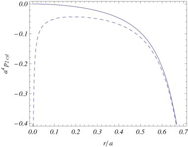
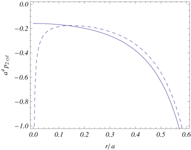
Figure 2: The effective azimuthal pressure induced by the cylindrical shell on the wedge sides, $a^{4}p_{2\mathrm{cyl}}$, as a function of $r/a$ for Dirichlet scalar (left panel) and for the electromagnetic field (right panel). The full (dashed) curves correspond to $q=2$ ($q=2/3$).

Now, let us discuss the behavior of the boundary-induced part in the VEV of the energy-momentum tensor in the asymptotic regions of the parameters. Near the cylindrical shell the main contribution comes from large values of $n$ and for the points $a-r\ll a|\sin\phi|,a|\sin(\phi_{0}-\phi)|$ the leading terms are the same as those for a cylindrical shell when the wedge is absent. For points near the edges $(r=a,\phi=0,\phi_{0})$ the leading terms in the corresponding asymptotic expansions are the same as for the geometry of a wedge with the opening angle $\phi_{0}=\pi/2$. Near the edge, $r\rightarrow 0$, for the components (no summation over $i$) $\langle T_{i}^{i}\rangle_{\mathrm{cyl}}$, $i=0,3$, the main contribution comes from the mode $n=0$ and we find $\langle T_{i}^{i}\rangle_{\mathrm{cyl}}\approx-0.0590q/a^{4}$, $i=0,3$. For the components (no summation over $i$) $\langle T_{i}^{i}\rangle_{\mathrm{cyl}}$, $i=1,2$, when $q>1$ the main contribution again comes form $n=0$ term and one has $\langle T_{i}^{i}\rangle_{\mathrm{cyl}}\approx-\langle T_{0}^{0}\rangle_{\mathrm{cyl}}$, $i=1,2$. For $q<1$ the main contribution into the components $\langle T_{i}^{i}\rangle_{\mathrm{cyl}}$, $i=1,2$, comes from the term $n=1$ and we have (no summation over $i$) $\langle T_{i}^{i}\rangle_{\mathrm{cyl}}\varpropto r^{2(q-1)}$, $i=1,2$. In this case the radial and azimuthal stresses induced by the cylindrical shell diverge on the edge $r=0$. For the off-diagonal component the main contribution comes from the $n=1$ mode and $\langle T_{2}^{1}\rangle_{\mathrm{cyl}}$ behaves like $r^{2q-1}$.

Now we turn to the VEVs of the energy-momentum tensor in the exterior region. Subtracting from these VEVs the corresponding expression for the wedge without the cylindrical boundary, analogously to the case of the field square, it can be seen that the VEVs are presented in the form (64), with the parts induced by the cylindrical shell given by the formulae (no summation over $i$)

$$\langle T_{i}^{i}\rangle_{\mathrm{cyl}} = \frac{q}{2\pi^{2}}\sideset{}{{}^{\prime}}{\sum}_{n=0}^{\infty}\sum_{\lambda=0,1}\int_{0}^{\infty}dxx^{3}\frac{I_{qn}^{(\lambda)}(xa)}{K_{qn}^{(\lambda)}(xa)}F^{(i)}[\Phi_{qn}^{(\lambda)}(\phi),K_{qn}(xr)],$$ (72)

$$\langle T_{2}^{1}\rangle_{\mathrm{cyl}} = \frac{q^{2}}{4\pi^{2}}\frac{\partial}{\partial r}\sideset{}{{}^{\prime}}{\sum}_{m=0}^{\infty}n\sin(2qn\phi)\sum_{\lambda=0,1}(-1)^{\lambda}\int_{0}^{\infty}dxx\frac{I_{qn}^{(\lambda)}(xa)}{K_{qn}^{(\lambda)}(xa)}K_{qn}^{2}(xr).$$ (73)

Here the functions $F^{(i)}\left[\Phi(\phi),f(y)\right]$ are defined by expressions (67). It can be seen that the vacuum energy density induced by the cylindrical shell in the exterior region is positive.

In the way similar to that for the interior region, the force acting on the wedge sides is presented in the form of the sum (69), where for the part due to the presence of the cylindrical shell we have

$$p_{2\mathrm{cyl}}=-\langle T_{2}^{2}\rangle_{\mathrm{cyl}}|_{\phi=0,\phi_{0}}=-\frac{q}{\pi^{2}}\sideset{}{{}^{\prime}}{\sum}_{n=0}^{\infty}\sum_{\lambda=0,1}\int_{0}^{\infty}dxx^{3}\frac{I_{qn}^{(\lambda)}(xa)}{K_{qn}^{(\lambda)}(xa)}F_{qn}^{(\lambda)}[K_{qn}(xr)].$$ (74)

In this formula, the function $F_{\nu}^{(\lambda)}\left[f(y)\right]$ is defined by relations (71) and the corresponding forces are always attractive.

The leading divergence in the boundary induced part (72) on the cylindrical surface is given by the same formulae as for the interior region. For large distances from the shell and for $q>1$ the main contribution into the VEVs of the diagonal components comes from the $n=0$, $\lambda=1$ term and one has (no summation over $i$)

$$\langle T_{i}^{i}\rangle_{\mathrm{cyl}}\approx-\frac{qc_{i}\left(a/r\right)^{2}}{15\pi^{2}r^{4}},\;c_{0}=c_{3}=2,\;c_{1}=1,\;c_{2}=-5.$$ (75)

In the case $q<1$ the main contribution into the VEVs of the diagonal components at large distances from the cylindrical shell comes from the $n=1$ mode. The leading terms in the corresponding asymptotic expansions are given by the formulae

$$\langle T_{i}^{i}\rangle_{\mathrm{cyl}}\approx-q^{2}(q+1)c_{i}(q)\frac{\cos(2q\phi)}{\pi^{2}r^{4}}\left(\frac{a}{r}\right)^{2q},$$ (76)

with the notations

$$c_{0}(q)=c_{3}(q)=\frac{1}{2q+3},\;c_{1}(q)=\frac{2q^{2}+q+1}{(2q+1)(2q+3)},\;c_{2}(q)=-\frac{q+1}{2q+1}.$$ (77)

In the case $q=1$ the asymptotic terms are determined by the sum of the contributions coming from the modes $n=0$ and $n=1$. The latter are given by formulae (75), (76). For the off-diagonal component, for all values $q$ the main contribution at large distances comes from the $n=1$ mode and $\langle T_{2}^{1}\rangle_{\mathrm{cyl}}\varpropto(a/r)^{2q}r^{-3}$.

7 Conclusion

We have investigated the polarization of the scalar and electromagnetic vacua by a wedge with coaxial cylindrical boundary, assuming Dirichlet boundary conditions in the case of a scalar field and perfectly conducting boundary conditions for the electromagnetic field. The application of the Abel-Plana-type summation formula for the series over the zeros of the Bessel function and its derivative allowed us to extract from the VEVs the parts due to the wedge without a cylindrical boundary and to present the additional parts induced by this boundary in terms of exponentially convergent integrals. The vacuum densities for the geometry of a wedge without a cylindrical boundary are considered in section 3. We have derived formulae for the renormalized VEVs of the field squared and the energy-momentum tensor, formulae (22), (24). For a conformally coupled scalar the energy-momentum tensor is diagonal and does not depend on the angular variable $\phi$. The corresponding vacuum forces acting on the wedge sides are attractive for $\phi_{0}<\pi$ and are repulsive for $\phi_{0}>\pi$.

For a scalar field the parts in the Wightman function induced by the cylindrical boundary are given by formulae (13) and (17) for the interior and exterior regions respectively. The corresponding VEVs for the field squared and the energy-momentum tensor are investigated in section 4. The field squared is given by formula (33) and vanishes on the wedge sides $\phi=\phi_{m}$ for all points away from the cylindrical surface. The energy-momentum tensor induced by the cylindrical surface is non-diagonal and the corresponding components are determined by formulae (35), (36). The off-diagonal component vanishes on the wedge sides. The additional vacuum forces acting on the wedge sides due to the presence of the cylindrical surface are determined by the ${}_{2}^{2}$-component of the corresponding stress and are attractive for all values $\phi_{0}$. On the wedge sides the corresponding vacuum stresses in the directions parallel to the wedge sides are isotropic and the energy density is negative for both minimally and conformally coupled scalars. The formulae in the exterior region differ from the corresponding formulae for the interior region by the interchange $I_{qn}(z)\leftrightarrows K_{qn}(z)$. For large distances from the cylindrical surface, $r\gg a$, the VEVs behave as $(a/r)^{D-1+2q}$ for the field squared and as $(a/r)^{D+1+2q}$ for the diagonal components of the energy-momentum tensor.

In the second part of the paper we have evaluated the VEVs of the field squared and the energy-momentum tensor for the electromagnetic field. For the wedge without the cylindrical shell the VEVs of the field squared are presented in the form (54). The first term on the right of this formula corresponds to the VEVs for the geometry of a cosmic string with the angle deficit $2\pi-\phi_{0}$. The parts induced by the cylindrical shell are presented in the form (51) for the interior region and in the form (58) for the exterior region. We have discussed these general formulae in various asymptotic regions of the parameters. In section 6 we consider the VEV of the energy-momentum tensor. For the geometry of a wedge without the cylindrical boundary the vacuum energy-momentum tensor does not depend on the angle $\phi$ and is the same as in the geometry of the cosmic string. The corresponding vacuum forces acting on the wedge sides are attractive for $\phi_{0}<\pi$ and repulsive for $\phi_{0}>\pi$. In particular, the equilibrium position corresponding to the geometry of a single plate is unstable. For the region inside the shell the part in the VEV of the energy-momentum tensor induced by the presence of the cylindrical shell is non-diagonal and the corresponding components are given by formulae (65), (66) for the interior region and by (72), (73) for the exterior region. The vacuum energy density induced by the cylindrical shell is negative in the interior region and is positive in the exterior region. For a wedge with $\phi_{0}<\pi$ the part in the vacuum energy-momentum tensor induced by the shell is finite on the edge $r=0$. For $\phi_{0}>\pi$ the shell-induced parts in the energy density and the axial stress remain finite, whereas the radial and azimuthal stresses diverge as $r^{2(\pi/\phi_{0}-1)}$. The corresponding off-diagonal component behaves like $r^{2\pi/\phi_{0}-1}$ for all values $\phi_{0}$. For points near the edges $(r=a,\phi=0,\phi_{0})$, the leading terms in the corresponding asymptotic expansions are the same as for the geometry of a wedge with the opening angle $\phi_{0}=\pi/2$. The presence of the shell leads to additional forces acting on the wedge sides. The corresponding effective azimuthal pressures are given by formulae (70), (74) and these forces are always attractive.

References

• [1] H.B.G. Casimir, Proc. K. Ned. Akad. Wet. 51, 793 (1948).
• [2] V.M. Mostepanenko and N.N. Trunov, The Casimir Effect and Its Applications (Oxford University Press, Oxford, 1997 ).
• [3] E. Elizalde, S.D. Odintsov, A. Romeo, A.A. Bytsenko, and S. Zerbini, Zeta Regularization Techniques with Applications (World Scientific, Singapore, 1994); M. Bordag, U. Mohidden, and V.M. Mostepanenko, Phys. Rep. 353, 1 (2001); K.A. Milton The Casimir Effect: Physical Manifestation of Zero-Point Energy (World Scientific, Singapore, 2002); V.V. Nesterenko, G. Lambiase, and G. Scarpetta, Riv. Nuovo Cim. 27, No. 6, 1 (2004).
• [4] P.M. Fishbane, S.G. Gasiorowich, and P. Kauss, Phys. Rev. D 36, 251 (1987); P.M. Fishbane, S.G. Gasiorowich, and P. Kauss, Phys. Rev. D 37, 2623 (1988); B.M. Barbashov and V.V. Nesterenko, Introduction to the Relativistic String Theory (World Scientific, Singapore, 1990).
• [5] J. Ambjørn and S. Wolfram, Ann. Phys. 147, 1 (1983).
• [6] L.L. De Raad Jr. and K.A. Milton, Ann. Phys. 136, 229 (1981).
• [7] K.A. Milton, A.V. Nesterenko, and V.V. Nesterenko, Phys. Rev. D 59, 105009 (1999); P. Gosdzinsky and A. Romeo, Phys. Lett. B 441, 265 (1998); G. Lambiase, V.V. Nesterenko, and M. Bordag, J. Math. Phys. 40, 6254 (1999).
• [8] I. Cavero-Peláez and K.A. Milton, J. Phys. A 39, 6225 (2006); A. Romeo and K.A. Milton, J. Phys. A 39, 6225 (2006); I. Brevik and A. Romeo, Physics Scripta 76, 48 (2007).
• [9] A.A. Saharian, Izv. AN Arm. SSR. Fizika 23, 130 (1988) [Sov. J. Contemp. Phys. 23, 14 (1988)].
• [10] A.A. Saharian, Dokladi AN Arm. SSR 86, 112 (1988) (Reports NAS RA, in Russian).
• [11] A.A. Saharian, hep-th/0002239.
• [12] F.D. Mazzitelli, M.J. Sanchez, N.N. Scoccola, and J. von Stecher, Phys. Rev. A 67, 013807 (2002); D.A.R. Dalvit, F.C. Lombardo, F.D. Mazzitelli, and R. Onofrio, Europhys. Lett. 67, 517 (2004); F.D. Mazzitelli, in Quantum Field Theory under the Influence of External Conditions, ed. by K. A. Milton (Rinton Press, Princeton NJ, 2004); D.A.R. Dalvit, F.C. Lombardo, F.D. Mazzitelli, and R. Onofrio, Phys. Rev. A 74, 020101(R) (2006); F.D. Mazzitelli, D.A.R. Dalvit, and F.C. Lombardo, New J. Phys. 8, 240 (2006); F.C. Lombardo, F.D. Mazzitelli, and P.I. Villar, arXiv:0808.3368.
• [13] A. Romeo and A.A. Saharian, Phys. Rev. D 63, 105019 (2001).
• [14] A.A. Saharian and A.S. Tarloyan, J. Phys. A 39, 13371 (2006).
• [15] A.R. Kitson and A. Romeo, Phys. Rev. D 74, 085024 (2006).
• [16] V.N. Marachevsky, Phys. Rev. D 75, 085019 (2007).
• [17] G.L. Klimchitskaya, E.V. Blagov,  and V. M. Mostepanenko, J. Phys. A 39, 6481 (2006); T. Emig, R.L. Jaffe, M. Kardar, and A. Scardicchio, Phys. Rev. Lett. 96, 080403 (2006); M. Bordag, Phys.Rev. D 73, 125018 (2006); H. Gies and K. Klingmuller, Phys. Rev. Lett. 96, 220401 (2006); H. Gies and K. Klingmuller, Phys.Rev. D 74, 045002 (2006); K.A. Milton and J. Wagner, arXiv:0711.0774; S.J. Rahi, A.W. Rodriguez, T. Emig, R.L. Jaffe, S.G. Johnson, and M. Kardar, Phys. Rev. A 77, 030101(R) (2008); I. Cavero-Pelaez, K.A. Milton, P.Parashar, and K.V. Shajesh, arXiv:0805.2777; S.J. Rahi, T. Emig, R.L. Jaffe, and M. Kardar, arXiv:0805.4241; A.W. Rodriguez, J.N. Munday, J.D. Joannopoulos, F. Capasso, D.A.R. Dalvit, and arXiv:0807.4166; S.G. Johnson, M. Schaden, arXiv:0808.3966; M. Schaden, arXiv:0810.1046; I. Cavero-Pelaez, K.A. Milton, P. Parashar, and K.V. Shajesh, arXiv:0810.1786.
• [18] J.S. Apps and J.S. Dowker, Class. Quantum Grav. 15, 1121 (1998); J.S. Dowker, Divergences in the Casimir energy, hep-th/0006138; V.V. Nesterenko, I.G. Pirozhenko, and J. Dittrich, Class. Quantum Grav. 20, 431 (2003).
• [19] J.S. Dowker and G. Kennedy, J. Phys. A 11, 895 (1978).
• [20] D. Deutsch and P. Candelas, Phys. Rev. D 20, 3063 (1979).
• [21] I. Brevik and M. Lygren, Ann. Phys. 251, 157 (1996).
• [22] I. Brevik, M. Lygren, and V.N. Marachevsky, Ann. Phys. 267, 134 (1998).
• [23] I. Brevik and K. Pettersen, Ann. Phys. 291, 267 (2001).
• [24] V.V. Nesterenko, G. Lambiase, and G. Scarpetta, Ann. Phys. 298, 403 (2002).
• [25] H. Gies and K. Klingmuller, Phys. Rev. Lett. 97, 220405 (2006).
• [26] V.V. Nesterenko, G. Lambiase, and G. Scarpetta, J. Math. Phys. 42, 1974 (2001).
• [27] E.B. Kolomeisky1 and J.P. Straley, arXiv:0712.1974.
• [28] A.H. Rezaeian and A.A. Saharian, Class. Quantum Grav. 19, 3625 (2002).
• [29] A.A. Saharian and A.S. Tarloyan, J. Phys. A 38, 8763 (2005).
• [30] A.A. Saharian, Eur. Phys. J. C 52, 721 (2007).
• [31] A.A. Saharian and A.S. Tarloyan, Ann. Phys. 323, 1588 (2008).
• [32] I. Brevik and T. Toverud, Class. Quantum Grav. 12,1229 (1995); E.R. Bezerra de Mello, V.B. Bezerra, A.A. Saharian, and A.S. Tarloyan, Phys. Rev. D 74, 025017 (2006); E.R. Bezerra de Mello, V.B. Bezerra, and A.A. Saharian, Phys. Lett. B 645, 245 (2007); E.R. Bezerra de Mello, V.B. Bezerra, A.A. Saharian, and A.S. Tarloyan, arXiv:0809.0844.
• [33] A.A. Saharian, arXiv:0708.1187.
• [34] G. Kennedy, R. Critchley, and J.S. Dowker, Ann. Phys. 125, 346 (1980).
• [35] P. Candelas, Ann. Phys. 143, 241 (1982).
• [36] A.A. Actor and I. Bender, Fortschr. Phys. 44, 281 (1996).
• [37] A.D. Helfer and A.S.I.D. Lang, J. Phys. A 32, 1937 (1999); V. Sopova and L.H. Ford, Phys. Rev. D 66, 045026 (2002); G. Barton, J. Phys. A 38, 3021 (2005).