Dynamics and modulation of ring dark soliton in 2D Bose-Einstein
condensates with tunable interaction

Abstract

We investigate the dynamics and modulation of ring dark soliton in 2D Bose-Einstein condensates with tunable interaction both analytically and numerically. The analytic solutions of ring dark soliton are derived by using a new transformation method. For shallow ring dark soliton, it is stable when the ring is slightly distorted, while for large deformation of the ring, vortex pairs appear and they demonstrate novel dynamical behaviors: the vortex pairs will transform into dark lumplike solitons and revert to ring dark soliton periodically. Moreover, our results show that the dynamical evolution of the ring dark soliton can be dramatically affected by Feshbach resonance, and the lifetime of the ring dark soliton can be largely extended which offers a useful method for observing the ring dark soliton in future experiments.

I INTRODUCTION

Solitons are fundamental excitations of nonlinear media and have attracted great interests from diverse contexts of science and engineering, such as dynamics of waves in shallow water, transport along DNA and other macromolecules, and fiber optic communications. The realization of Bose-Einstein condensates (BECs) bec introduces an unparalleled platform for the study of these nonlinear excitations, where both bright bright and dark solitons Burger ; Denschlag ; Dutton ; Ginsberg ; Anderson have been observed. Very recently, quasi-1D dark solitons with long lifetime up to $2.8$s have been created in the laboratory Becker . This offers an unusual opportunity to study dark solitons and the relevant theories.

Dark solitons are robust localized defects in repulsive BECs, which are characterized by a notch in the condensate density and a phase jump across the center Kivshar2 . So far most of the works on dark soliton are limited to one-dimensional (1D) BECs (Gorlitz , for a review see Proukakis ; Sevrekidis ; Carretero ), where they are both stable and easily controlled in experiments. However, in two dimensions (2D), most types of dark solitons are short lived due to dynamical instability arising from higher dimensionality Denschlag . For example, in ref. huang it is shown that both 2D dark lumplike soliton and dark stripe soliton will decay into vortex pairs under small transverse perturbations. Also these 2D defects are strongly affected by inhomogeneity of the system and suffer from the snaking instability just as in optical systems (Tikhonenko ; Kivshar2 and references therein). Therefore their long-time dynamical behaviors are hard to observe in real experiments.

One candidate for observing the long-time behavior of 2D dark soliton is ring dark solitons (RDS) which was first introduced in the context of optics Kivshar ; Baluschev and then studied in BECs Theocharis . In a 2D nonlinear homogeneous system, it was first predicted that the instability band of a dark stripe soliton can be characterized by a maximum perturbation wavenumber $Q_{max}$ Kuznetsov ; and if the length of the stripe is smaller than the inverse of the wavenumber $L<2\pi/Q_{max}$, then the stripe can be bent into an annulus with the instability being largely suppressed. This was further confirmed for BECs even in an inhomogeneous trap, where both oscillatory and stationary ring dark solitons can exist Theocharis . Besides, the symmetry of the ring soliton determines that it is little affected by the inhomogeneity of BEC system. Moreover, the study indicated that the collisions between the RDSs are quasielastic and their shapes will not be distorted Nistazakis . Due to these specific characteristics of the RDS, it has stimulated great interests on observing 2D dark solitons in BECs Carr ; xue ; Theocharis3 ; Dong . Recently, Yang et al. suggested a proposal on how to create the RDSs in experiment yang . Nevertheless, the generation of the RDS and their dynamical behaviors in BECs have not been observed in real experiment yet. This is because the lifetime of deep RDS is not long enough for the experimental observation and the stability analysis for shallow RDS has not been explored thoroughly.

In this paper, we first develop a general effective analytical method to derive the solutions of RDS. This is realized by transforming the Gross-Pitaevskii (GP) equation with trap potential to a standard nonlinear Schrödinger (NLS) equation. Then we numerically solve the 2D GP equation and obtain a stability diagram where a stable domain of shallow RDSs can exist. In the unstable region, we find a novel transformation process between various dark solitons and vortex pairs. Finally, we show that the lifetime of RDSs can be largely extended by Feshbach resonance, which is of particular importance for the experimental observation of RDSs.

II The Model

A BEC trapped in an external potential is described by a macroscopic wave function $\Psi(\textbf{r},t)$ obeying the GP equation Dalfovo , which reads

$$i\hbar\frac{\partial\Psi(\textbf{r},t)}{\partial t}\!=\![-\frac{\hbar^{2}}{2m}\nabla^{2}\!+\!V(\textbf{r},t)\!+\!g_{0}(t)\mid\Psi(\textbf{r},t)\mid^{2}]\Psi(\textbf{r},t),$$

where the wave function is normalized by the particle number $N=\int d\textbf{r}\mid\Psi\mid^{2}$ and $g_{0}(t)=4\pi\hbar^{2}a(t)/m$ represents the strength of interatomic interaction characterized by the $s$ -wave scattering length $a(t)$, which can be tuned by Feshbach resonance. The trapping potential is assumed to be $V(\textbf{r},z)=m(\omega_{r}^{2}r^{2}+\omega_{z}^{2}z^{2})/2$, where $r^{2}=x^{2}+y^{2}$, $m$ is the atom mass, and $\omega_{r,z}$ are the confinement frequencies in the radial and axial directions respectively. Further assuming $\Omega\equiv\omega_{r}/\omega_{z}\ll 1$ such that the motion of atoms in the $z$ direction is essentially frozen to the ground state ($f(z)$) of the axial harmonic trapping potential, the system can be regarded as quasi-2D. Then we can separate the degrees of freedom of the wave function as $\Psi(\textbf{r},t)=\psi(x,y,t)f(z)$, obtaining the 2D GP equation:

$$i\hbar\frac{\partial\psi}{\partial t}=-\frac{\hbar^{2}}{2m}(\frac{\partial^{2}}{\partial x^{2}}+\frac{\partial^{2}}{\partial y^{2}})\psi\!+\!\frac{m}{2}\omega_{r}^{2}r^{2}\psi\!+\!g_{0}(t)\eta\mid\psi\mid^{2}\psi,$$

where

$$\eta\equiv\frac{\int dz\mid f(z)\mid^{4}}{\int dz\mid f(z)\mid^{2}}.$$

It is convenient to introduce the scales characterizing the trapping potential: the length, time, and wave function are scaled as

$$x=a_{h}\tilde{x},t=\frac{\tilde{t}}{\omega_{z}},\psi=\frac{\tilde{\psi}}{a_{h}\sqrt{4\pi a_{0}\eta}}$$

respectively, with $a_{h}=\sqrt{\hbar/m\omega_{z}}$ and $a_{0}$ is a constant length we choose to measure the time-dependent $s$ -wave scattering length. Then the 2D GP equation is reduced to a dimensionless form as

$$i\frac{\partial\psi}{\partial t}=-\frac{1}{2}\nabla^{2}\psi+g(t)\mid\psi\mid^{2}\psi+\frac{1}{2}\Omega^{2}r^{2}\psi,$$ (1)

where $\nabla^{2}=\partial^{2}/\partial x^{2}+\partial^{2}/\partial y^{2}=\partial^{2}/\partial r^{2}+1/r\times\partial/\partial r+\partial^{2}/\partial\theta^{2}$, $\Omega=\omega_{r}/\omega_{z}$, $g(t)=a(t)/a_{0}$ and the tilde is omitted for simplicity. This is the basic equation we treat analytically and numerically.

III transformation method and analytic Solution

In order to study the dynamics of ring dark soliton, we consider the solution of Eq. (1) with circular symmetry, $\psi(r,t)$. In the case of $g(t)=C$, where $C$ is a nonzero positive constant, the main difficulty to solve Eq. (1) is the existence of the last term, i.e. the trapping potential. Without trap, i.e. $\Omega=0$, the system is described by the standard NLS equation:

$$i\frac{dQ(R,T)}{dT} + \frac{1}{2}(\frac{\partial^{2}Q(R,T)}{\partial R^{2}}+\frac{1}{R}\frac{\partial Q(R,T)}{\partial R})$$ (2)

$$- C\mid Q(R,T)\mid^{2}Q(R,T)=0,$$

Under small-amplitude approximation, Eq. (2) has been transformed to the famous cylindrical KdV (cKdV) equation by using the perturbation method Kivshar ; xue . The cKdV equation is known to be basic nonlinear equation describing cylindrical and spherical pulse solitons in plasmas, electric lattices and fluids (see, e.g., Infeld for a review) and its exact solution has been derived ckdv . Therefore the soliton solutions of Eq. (2) are gained.

However, there is no effective method to solve Eq. (1) generally, especially when the last term is time-dependent, $V(t)$. Now we develop a method which can transform the general form of Eq. (1) to Eq. (2) by using a transformation:

$$\psi(r,t)=Q(R(r,t),T(t))e^{ia(r,t)+c(t)},$$ (3)

where $R(r,t)$, $T(t)$, $a(r,t)$, and $c(t)$ are assumed to be real functions and the transformation parameters read

$$R(r,t) = \alpha(t)r,$$

$$T(t) = \int\alpha^{2}(t^{\prime})dt^{\prime}+C_{0},$$

$$c(t) = \frac{1}{2}\ln\frac{\alpha^{2}(t)}{C},$$

$$a(r,t) = -\frac{1}{2\alpha(t)}\frac{d\alpha(t)}{dt}r^{2},$$ (4)

where $C_{0}$ is a constant. The condition that such transformations exist is

$$\frac{1}{\alpha(t)}\frac{d^{2}\alpha(t)}{dt^{2}}-\frac{2}{\alpha(t)^{2}}(\frac{d\alpha(t)}{dt})^{2}-\Omega^{2}=0.$$ (5)

Under this condition, all solutions of Eq. (2) can be recast into the corresponding solutions of Eq. (1). So we build a bridge between the extensive RDS study in nonlinear optics (homogeneous system) and the trapped BEC system. Furthermore, it is worth while to note that the transformation method can be used to solve the general equation:

$$i \frac{du(r,t)}{dt}+D(t)(\frac{\partial^{2}u(r,t)}{\partial r^{2}}+\frac{1}{r}\frac{\partial u(r,t)}{\partial r})$$ (6)

$$+ g(t)\mid u(r,t)\mid^{2}u(r,t)+V(t)r^{2}u(r,t)=0,$$

when $g(t)$ is proportional to $D(t)$. Eq. (6) completely describes the dynamics and modulation of both electric field in optical systems and macroscopic order parameter in atomic BECs in quasi-2D with circular symmetry.

In order to get the transformation condition explicitly, we substitute $y(t)=d\alpha/(\alpha dt)$ into Eq. (5) and obtain

$$\frac{dy(t)}{dt}=y^{2}+\Omega^{2}.$$ (7)

This is a standard Riccati equation. We can solve it not only for $\Omega=constant$, but also for various type of $\Omega^{2}(t)$, such as $a+bsin(\lambda t)$, $a+bcosh(t)$, $ae^{\lambda t}$ ($a$, $b$, $\lambda$ are arbitrary constants) and so on. Thus we can study the dynamics of system with time-dependent external trap. Particularly, when $\Omega$ is independent on $t$, the solution of Eq. (5) is

$$\alpha(t)=C_{1}\sec(\Omega t+C_{2}),$$ (8)

where $C_{1}$ and $C_{2}$ are the integral constants.

Since under small-amplitude approximation, the solutions of Eq. (2) have been given, then combining the solutions of Eqs. (2) and (8), we get the corresponding solutions of RDS in the BEC in the external trap potential. They are the exact solutions of system when the depth of RDS is infinitely small, which help us to understand the dynamics of RDS. However, when the RDSs get deeper, the small-amplitude approximation is invalid and we have to appeal to the numerical simulation. In the following sections, we study the dynamics and stability of RDS numerically.

IV Stability of shallow ring dark soliton

It has been known that starting from the initial configuration with strict circular symmetry, the RDS will oscillate up to a certain time till instabilities develop: shallow RDS slowly decays into radiation and for deep one, snaking sets in, leading to formation of vortex-antivortex pairs arranged in a robust ringshaped array (vortex cluster), because of transverse perturbations Theocharis . But its stability to the perturbation in the radial direction is not analyzed. Here we study the stability of shallow RDS against the small distortion of the ringshape numerically, which is ineluctable in the process of the practical experiment.

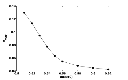
FIG. 1: A part of stability diagram of shallow ring dark soliton with $R_{0}=28.9$ and the trap frequency $\Omega=0.028$. The maximum eccentricity $e_{max}$ of the ring in the initial configuration decreases as the initial depth $\cos\phi(0)$ of the ring dark soliton increases.

We study the stability of RDSs by solving Eq. (1) numerically with the parameter: $g(t)=1$, $\Omega=0.028$ and the initial radius of RDS $R_{0}=28.9$. Because of large initial radius, a reasonable and good approximation is

$$\psi(x,y,0) = (1-\Omega^{2}r^{2}/4)$$ (9)

$$\times \left[\cos\phi(0)\tanh Z(r_{1})+i\sin\phi(0)\right],$$

where $r=\sqrt{x^{2}+y^{2}}$, $Z(r_{1})=(r_{1}-R_{0})\cos\phi(0)$, $r_{1}=\sqrt{(1-e_{c}^{2})x^{2}+y^{2}}$, $e_{c}$ is the eccentricity of the ring and $\cos\phi(0)$ is proportional to the depth of the input soliton. When $e_{c}\neq 0$, $R_{0}$ represents the length of semiminor axis of the elliptical configuration. We take Eq. (9) as the initial configuration, the validity of which has been explained in detail and checked in the previous investigations Theocharis ; Kivshar .

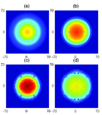
FIG. 2: (Color online) Evolution of the ring dark soliton with initial depth $\cos\phi(0)=0.6$, eccentricity $e_{c}=0.4$, interaction strength $g(t)=1$ and the trap frequency $\Omega=0.028$. (a) The initial profile shown by color-scale density plots, where ring dark soliton corresponds a light-color plot ellipse with the length of semiminor axis $R_{0}=28.9$. (b)-(d) correspond to $t=80$, 400, 540 respectively. The ring dark soliton with distortion firstly breaks into two lump solitons, and then two pairs of vortex pairs. See text for details.

We propagate the 2D time-dependent GP equation (Eq. (1)) using two distinct techniques: alternating-direction implicit method Press ; Kasamatsu and time-splitting Fourier spectral method bao . The results from these two methods are crosschecked and When $e_{c}=0$, the properties of results are in agreement with those in Theocharis very well.

To translate the results into units relevant to the experiment Burger ; Denschlag , we assume a ${}^{87}Rb$ ($a_{0}=5.7$ nm) condensate of radius $30$ $\mu m$, containing $20000$ atoms in a disk-shaped trap with $\omega_{r}=2\pi\times 18$ Hz and $\omega_{z}=2\pi\times 628$ Hz. In this case, the RDS considered above has the radius $R_{0}=12.38$ $\mu m$, and the unit of time is $0.25$ ms.

Our numerical results show that the shallow RDS (refers to $\cos\phi(0)<0.67$, where the soliton without distortion will not suffer from the snaking instability) is stable against the small distortion of the ringshape. There is a maximum eccentricity $e_{max}$ for a given initial depth. When $e_{c}<e_{max}$, the RDSs are stable and oscillate reserving their shape with the same period as the unperturbed RDSs until decaying out. The $e_{max}$ becomes smaller with the initial depth increasing (see Fig. 1). This is because $2\pi/Q_{max}$ decreases as the RDS becomes deeper Kivshar , thus the shallower RDS can support larger distortion.

When $e_{c}$ exceeds $e_{max}$, snaking sets in and the dark soliton breaks into two vortex pairs, presenting a striking contrast to the multiples of four pairs reported previously. And the evolution of vortex pair is very different from the case of the deep RDSs without distortion.

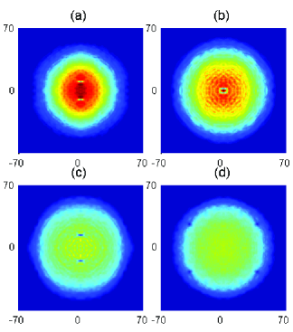
FIG. 3: (Color online) Evolution of vortex pairs following the Fig. 2 for (a) $t=640$, (b) $t=660$, (c) $t=680$ and (d) $t=1000$. The vortex pairs collide and merge into dark lumplike solitons, which move, then form a ring dark soliton for a short time and revive. Finally the lumplike solitons again break into vortex pairs. See text for details.

To illustrate the generic scenarios, we take the typical case with $\cos\phi(0)=0.6$ and $e_{c}=0.4$. It initially shrinks and when reaching the minimum radius in the short-axis direction, it starts snaking and forming two dark lumplike solitons in the horizontal direction; they move in the opposite direction and then break into two vortex pairs (see Fig. 2(b)). The vortex pairs arrange themselves in a ring configuration which performs slow radial oscillations. Simultaneously the vortices and antivortices move along the ring (see Fig. 2(c, d)). The result of motion is their collision in pairs in the vertical direction, followed by vortices and antivortices’s mergence and totally forming a pair of lumplike solitons (see Fig. 3(a)), which process has been confirmed by phase distribution of the system. The lumplike solitons move towards to each other, i.e. to the center of condensate, in the vertical direction. When they reach the minimum radius, a ring dark soliton forms (see Fig. 3(b)). After a short time the system returns to the state of two dark lumplike solitons. The lumplike solitons leave each other (see Fig. 3(c)) and in the path, each of lumplike solitons breaks into a vortex pair again. But the configuration is different to the initial one: the vortex (antivortex) is substituted by antivortex (vortex), just like the vortex and the antivortex passing each other directly following the motion before the mergence. Then the vortices and the antivortices keep on moving (see Fig. 3(d)), then collide and merge in the horizontal direction. The dynamical process repeats itself.

This dynamical behavior of the vortex pairs is novel and part of the process is similar to the behavior of lump soliton reported in huang . The certain centrical collision of vortex pair provides a potential tool to study the collision dynamics of vortices.

V controlling of deep ring dark solitons

The deep ring dark solitons (refer to $\cos\phi(0)>0.67$) suffer from the snaking instability and can only survive for a short time (typically $10$ ms in the numerical simulation) before changing into other soliton type. Longer lifetime is necessary for the practical observation of complex soliton physics such as oscillations or collisions Becker . Our results show that the Feshbach resonance management technique can largely extend the lifetime of the ring dark solitons, which makes it possible to study the long-time behavior of 2D dark soliton in experiment.

Feshbach resonance Inouye is a quite effective mechanism that can be used to manipulate the interatomic interaction (i.e. the magnitude and sign of the scattering length), which has been used in many important experimental investigations, such as the formation of bright solitons bright . Feshbach resonance management refers to the time-periodic changes of magnitude and/or sign of scattering length by Feshbach resonance Kevrekidis , and has been widely used to modulate and stabilize bright solitons Ueda ; liu , while its effect on the dynamics and stability of dark soliton is not very definite Malomed . Taking the ring dark soliton as an example, we demonstrate that the Feshbach resonance can dramatically affect the dynamics of dark solitons.

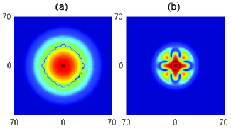
FIG. 4: (Color online) The snapshots of condensate with ring dark soliton under the Feshbach resonance management. The parameter are given as follow: (a) $e_{c}=0$, $\cos\phi(0)=1$, $g(t)=2-\sin(2\Omega t)$ and $t=60$ ($\approx 15$ ms); (b) $e_{c}=0$, $\cos\phi(0)=1$, $g(t)=e^{-\Omega t}$ and $t=100$ ($\approx 25$ ms). Other parameters are the same as Fig. 2. In the former case the ring dark soliton will break into $20$ vortex pairs, while only $4$ vortex pairs in the later one. The total atom number is the same in these two plot, so for clearness, we use different color scale.

To show the effect of Feshbach resonance management, Eq. (1) is integrated numerically with eccentricity $e_{c}=0$ and a time dependent nonlinear coefficient $g(t)$; other parameters and the initial condition are the same as in Sec. IV. We consider the cases of $g(t)\sim ae^{\pm\omega t}$ and $g(t)\sim a\pm\sin(\omega t)$, where $a$ and $\omega$ are arbitrary constant parameters. Our results show that for the deep ring dark solitons, the Feshbach resonance management remarkably changes the evolution and the instability of solitons, indicated by the number of vortex pairs which arise due to the snaking instability. Two typical examples are shown in Fig. 4: in the former one, the black ring dark solitons (refer to $\cos\phi(0)=1$) break into $20$ vortex pairs, while the latter one only has $4$ pairs. These phenomena are very different from those with constant scattering length which have $16$ vortex pairs. This makes it possible to study the dynamics of snaking instability in detail. What is more interesting and more important are the cases in which the lifetime of the RDS can be extended, such as $g(t)=1-\sin(\Omega t)$, as discussed below.

When the system subjects to the modulation of $g(t)=1-\sin(\Omega t)$, the RDS can exist for longer time before breakup. For example, when $\cos\phi(0)=0.76$, the lifetime can be extended up to $45$ ms from $10$ ms, in which process, we can observe one complete cycle of oscillation of RDS. While if we just reduce the scattering length but keeping it constant, the lifetime of RDS will not change much. For example, if $g(t)=0.2$, the RDS will become snaking at about $15$ ms. So the lifetime extension effect is due to the Feshbach resonance management. From Eq. (8), we can see that $\Omega$ is one intrinsic frequency of system. So it is reasonable to deduce that this effect is a resonance phenomenon. Furthermore, this effect is even valid for shallow RDS suffering from the instability due to the distortion of ringshape. It has been check that under Feshbach resonance management $g(t)=1-\sin(\Omega t)$, the RDS with $\cos\phi(0)=0.6$ and $e_{c}=0.4$, has a lifetime of $50$ ms, which is much larger than the original $10$ ms. Thus under large perturbation the RDS can exist long enough to be observed, which make the experimental study of RDS easier.

VI CONCLUSION

In conclusion, we have introduced a new transformation method to derive the solution of ring dark soliton, which provides a powerful analytic tool to study the 2D BECs and nonlinear optical systems with circular symmetry. Then we check the stability of shallow ring dark soliton, and find a novel dynamical behavior mode of solitons. Furthermore, we study the effect of Feshbach resonance management on the evolution and the stability of ring dark soliton, also discover a method to extend the lifetime of ring dark soliton largely. We show that the ring dark solition is a potential candidate for observing the long-time behavior of 2D dark soliton.

VII Acknowledgments

We acknowledge the heuristic discussion with Weizhu Bao. This work was supported by NSFC under grants Nos. 60525417, 10740420252, 10874235, the NKBRSFC under grants Nos. 2005CB724508 and 2006CB921400, and the Program for NCET.

References

- (1) M. H. Anderson, J. R. Ensher, M. R. Matthews, C. E. Wieman, E. A. Cornell, Science 269, 198 (1995); K. B. Davis, M. O. Mewes, M. R. Andrews, N. J. van Druten, D. S. Durfee, D. M. Kurn, and W. Ketterle, Phys. Rev. Lett. 75, 3969 (1995).
- (2) K. E. Strecker, G. B. Partridge, A. G. Truscott, and R. G. Hulet, Nature (London) 417, 150 (2002); L. Khaykovich, F. Schreck, G. Ferrari, T. Bourdel, J. Cubizolles, L. D. Carr, Y. Castin, C. Salomon, Science 296, 1290 (2002); S. L. Cornish, S. T. Thompson, and C. E. Wieman, Phys. Rev. Lett. 96, 170401 (2006).
- (3) S. Burger, K. Bongs, S. Dettmer, W. Ertmer, K. Sengstock, A. Sanpera, G. V. Shlyapnikov, and M. Lewenstein, Phys. Rev. Lett. 83, 5198 (1999).
- (4) J. Denschlag, J. E. Simsarian, D. L. Feder, C. W. Clark, L. A. Collins, J. Cubizolles, L. Deng, E. W. Hagley, K. Helmerson, W. P. Reinhardt, S. L. Rolston, B. I. Schneider, W. D. Phillips, Science 287, 97 (2000).
- (5) Z. Dutton, M. Budde, C. Slowe, L. V. Hau, Science 293, 663 (2001).
- (6) B. P. Anderson, P. C. Haljan, C. A. Regal, D. L. Feder, L. A. Collins, C. W. Clark, and E. A. Cornell, Phys. Rev. Lett. 86, 2926 (2001).
- (7) N. S. Ginsberg, J. Brand, and L. V. Hau, Phys. Rev. Lett. 94, 040403 (2005).
- (8) C. Becker, S. Stellmer, P. Soltan-Panahi, S. Dörscher, M. Baumert, E. Richter, J. Kronjäger, K. Bongs and K. Sengstock, Nature Phys. 4, 496 (2008).
- (9) Y. S. Kivshar, B. Luther-Davie, Phys. Rep. 298, 81 (1998).
- (10) A. Görlitz, J. M. Vogels, A. E. Leanhardt, C. Raman, T. L. Gustavson, J. R. Abo-Shaeer, A. P. Chikkatur, S. Gupta, S. Inouye, T. Rosenband, and W. Ketterle, Phys. Rev. Lett. 87, 130402(2001); J. Belmonte-Beitia, V. M. Pérez-García, V. Vekslerchik, and V. V. Konotop, Phys. Rev. Lett. 100, 164102 (2008); D. Zhao, X. G. He, and H. G. Luo, Arxiv: 0807.1192.
- (11) P. G. Kevrekidis, D. J. Frantzeskakis, R. Carretero-González, Ed., Emergent Nonlinear Phenomena in Bose-Einstein Condensates (Springer-Verlag, New York, 2008).
- (12) R. Carretero-González, D. J. Frantzeskakis and P. G. Kevrekidis, Nonlinearity 21, R139 (2008).
- (13) N. P. Proukakis, N. G. Parker, D. J. Frantzeskakis and C. S. Adams, J. Opt. B: Quantum Semiclass. Opt. 6, S380 (2004).
- (14) G. X. Huang, V. A. Makarov, and M. G. Velarde, Phys. Rev. A 67, 023604 (2003).
- (15) V. Tikhonenko, J. Christou, B. Luther-Davies, and Y. Kivshar, Opt. Lett. 21, 1129 (1996).
- (16) Y. S. Kivshar, X. P. Yang, Phys. Rev. E 50, R40 (1994); Chaos, Solitons and Fractals 4, 1745 (1994).
- (17) A. Dreischuh, D. Neshev, G. G. Paulus, F. Grasbon, and H. Walther, Phys. Rev. E 66, 066611 (2002).
- (18) G. Theocharis, D. J. Frantzeskakis, P. G. Kevrekidis, B. A. Malomed, and Y. S. Kivshar, Phys. Rev. Lett. 90, 120403 (2003).
- (19) E. Kuznetsov, S. Turitsyn, Zh. Eksp. Teor. Fiz. 94, 119 (1988) [Sov. Phys. JETP 67, 1583].
- (20) H. E. Nistazakis, D. J. Frantzeskakis, B. A. Malomed, P. G. Kevrekidis, Phys. Lett. A 285, 157 (2001).
- (21) L. D. Carr, and C. W. Clark, Phys. Rev. A 74, 043613 (2006).
- (22) G. Theocharis, P. Schmelcher, M. K. Oberthaler, P. G. Kevrekidis, and D. J. Frantzeskakis, Phys. Rev. A 72, 023609 (2005).
- (23) J. K. Xue, J. Phys. A: Math. Gen. 37, 11223 (2004); Eur. Phys. J. D 37, 241 (2006).
- (24) L. W. Dong, H. Wang, W. D. Zhou, X. Y. Yang, X. Lv, and H. Y. Chen, Opt. Exp. 16, 5649 (2008).
- (25) S. J. Yang, Q. S. Wu, S. N. Zhang, S. P. Feng, W. A. Guo, Y. C. Wen, and Y. Yu, Phys. Rev. A 76, 063606 (2007).
- (26) F. Dalfovo, S. Giorgini, L. P. Pitaevskii, and S. Stringari, Rev. Mod. Phys. 71, 463 (1999).
- (27) E. Infeld, G. Rowlands, Nonlinear Waves, Solitons and Chaos (Cambridge University Press, Cambridge, 1990).
- (28) R. Hirota, J. Phys. Soc. Jpn. 46, 1681 (1979); A. Nakamura, J. Phys. Soc. Jpn. 49, 2380 (1980); A. Nakamura, H. H. Chen, J. Phys. Soc. Jpn. 50, 711 (1981); R. S. Johnson, Wave Motion 30, 1 (1999); K. Ko and H. Kuehl, Phys. Fluids 22, 1343 (1979).
- (29) W. H. Press, S. A. Teukolsky, W. T. Vetterling, B. P. Flannery, Numerical Recipes in Fortran 77 (Cambridge University Press, Cambridge, 1992).
- (30) K. Kasamatsu, M. Tsubota, M. Ueda, Phys. Rev. A 67, 033610 (2003).
- (31) W. Z. Bao, D. Jaksch, P. A. Markowich, J. Comput. Phys. 187, 318 (2003).
- (32) S. Inouye, M. Andrews, J. Stenger, H. Miesner, D. Stamper-Kurn, W. Ketterle, Nature (London) 392, 151 (1998).
- (33) P. G. Kevrekidis, G. Theocharis, D. J. Frantzeskakis, and B. A. Malomed, Phys. Rev. Lett. 90, 230401 (2003).
- (34) H. Saito and M. Ueda, Phys. Rev. Lett. 90, 040403 (2003); F. Kh. Abdullaev, J. G. Caputo, R. A. Kraenkel, and B. A. Malomed, Phys. Rev. A 67, 013605 (2003).
- (35) Z. X. Liang, Z. D. Zhang, and W. M. Liu, Phys. Rev. Lett. 94, 050402 (2005); X. F. Zhang, Q. Yang, J. F. Zhang, X. Z. Chen, and W. M. Liu, Phys. Rev. A 77, 023613 (2008); B. Li, X. F. Zhang, Y. Q. Li, Y. Chen, and W. M. Liu, Phys. Rev. A 78, 023608 (2008).
- (36) B. A. Malomed, Soliton Management in Periodic Systems (Springer, New York, 2006).