Causal dissipative hydrodynamics obtained from the nonextensive/dissipative correspondence

Abstract

We derive the constitutive equations of causal relativistic dissipative hydrodynamics ($d$-hydrodynamics) from perfect nonextensive hydrodynamics ($q$-hydrodynamics) using the nonextensive/dissipative correspondence (NexDC) proposed by us recently. The $q$-hydrodynamics can be thus regarded as a possible model for the $d$-hydrodynamics facilitating its application to high energy multiparticle production processes. As an example we have shown that applying the NexDC to the perfect $1+1$ $q$-hydrodynamics, one obtains a proper time evolution of the bulk pressure and the Reynolds number.

The ideal hydrodynamic model successfully reproduces most of the RHIC experimental data Hirano0808.2684 suggesting that matter created there resembles a strongly interacting quark-gluon fluid TDLeeNPA750 rather than a free parton gas. However, there are also hints that, after all, a hadronic fluid cannot be totally ideal nonviscousindic and should be described by some kind of dissipative hydrodynamic model (or $d$-hydrodynamics) Eckart1940 ; HiscockPRD31 ; IsraelAnnPhys118 . A number of such models have been proposed recently MurongaPRC69 ; HeinzPRC73 ; BaierPRC73 ; KoidePRC75 ; ChaudhuriPRC74 . Although very promising, they have many difficulties, both in what concerns their proper formulation and applications HiscockPRD31 ; KoidePRC75 ; problems . Any new attempt to understand them more deeply is therefore welcome. In this letter we demonstrate that one can obtain constitutive equations of causal $d$-hydrodynamics starting from the relativistic perfect nonextensive hydrodynamics ($q$-hydrodynamics) supplemented by the nonextensive/dissipative correspondence (NexDC) proposed in OsadaPRC77 and taking place between the perfect $q$-hydrodynamics (based on the nonextensive Tsallis statistics Tsallis and described by the nonextensivity parameter $q$) and the usual $d$-hydrodynamics (based on the extensive Boltzmann-Gibbs statistics (BG) to which Tsallis statistics converges for $q\rightarrow 1$). We argue that the $d$-hydrodynamics emerging from such $q$-hydrodynamics is causal and preserves the simplicity of the latter which facilitates numerical applications OsadaPRC77 (instead of solving very complicated second order equations of $d$-hydrodynamics one can solve the much simpler equation of motion of the $q$-hydrodynamics).

Our $q$-hydrodynamics OsadaPRC77 is based on the relativistic nonextensive kinetic theory proposed in LavagnoPhysLettA301 (see also LimaPhysRevLett86 ). It is understood that such a theory accounts, by means of the parameter $q$, for all kinds of possible strong intrinsic fluctuations and long-range correlations existing in a hadronizing system. It replaces the usual notion of local thermal equilibrium by a kind of stationary state which also includes some interactions. It is described by the Tsallis nonextensive statistics Tsallis and characterized by the nonextensive parameter $q>1$ KodamaJPhys31 ; SR ; Biro . In this approach the perfect $q$-hydrodynamic equations (i.e., equations for the perfect nonextensive $q$-fluid without any additional currents) are given by the $q$-version of the energy momentum tensor:

$${\cal T}_{q;\mu}^{\mu\nu}=\Big{[}\varepsilon_{q}(T_{q})u_{q}^{\mu}u_{q}^{\nu}-P_{q}(T_{q})\Delta_{q}^{\mu\nu}\Big{]}_{;\mu}=0.$$ (1)

Here $\varepsilon_{q}(T_{q})$, $P_{q}(T_{q})$, $T_{q}=T_{q}(x)$ and $u^{\mu}_{q}(x)$ are, respectively, the nonextensive energy density, pressure and temperature field OsadaPRC77 and an accompanying hydrodynamic $q$-flow four vector field (which allows decomposition (1) to be performed; $\Delta_{q}^{\mu\nu}\equiv g^{\mu\nu}-u_{q}^{\mu}u_{q}^{\nu}$). If $T(x)$ and $u^{\mu}(x)$ are the corresponding temperature and velocity fields in the case of BG statistics ($q=1$) with $\varepsilon$ and $P$ being the usual energy density and pressure then, as proposed in OsadaPRC77 , one can map a $q$-flow into some dissipative $d$-flow by requiring that the following relations hold:

$$P(T)=P_{q}(T_{q}),\quad\varepsilon(T)=\varepsilon_{q}(T_{q})+3\Pi,$$ (2)

where $\Pi$ is to be regarded as the bulk pressure of $d$-hydrodynamics which is defined by

$$\Pi\equiv\frac{1}{3}w_{q}[\gamma^{2}+2\gamma].$$ (3)

Here $\delta u_{q}^{\mu}\equiv u_{q}^{\mu}-u^{\mu}$ is the four velocity difference between the non-extensive parameter $q>1$ and $q=1$ flows, $\gamma(x)\equiv\delta u_{q}^{\mu}(x)u_{\mu}(x)=-\frac{1}{2}\delta u_{q\mu}\delta u_{q}^{\mu}$ and $w_{q}\equiv\varepsilon_{q}+P_{q}$ is the $q$-enthalpy. If $T(x)$ and $\gamma(x)$ satisfy Eq. (2) relations in the whole space-time region, one can always transform equation of perfect $q$-hydrodynamics Eq. (1) into the following equation of $d$-hydrodynamics Eckart1940 ; HiscockPRD31 ; IsraelAnnPhys118 ; MurongaPRC69 ; HeinzPRC73 ; BaierPRC73 ; KoidePRC75 ; ChaudhuriPRC74 :

$$\left[\varepsilon(T)u^{\mu}u^{\nu}\!-\!\left[P(T)+\Pi\right]\Delta^{\mu\nu}\!\!\!+\!2W^{(\mu}u^{\nu)}\!+\!\pi^{\mu\nu}\right]_{;\mu}\!\!\!\!=0,$$ (4)

in which one recognizes the energy flow vector $W^{\mu}$ and the (symmetric and traceless) shear pressure tensor $\pi^{\mu\nu}$,

$$W^{\mu}=w_{q}[1+\gamma]\Delta^{\mu}_{\sigma}\delta u_{q}^{\sigma},\quad\pi^{\mu\nu}=w_{q}\delta u_{q}^{<\mu}\delta u_{q}^{\nu>}$$ (5)

(where $\Delta^{\mu\nu}\equiv g^{\mu\nu}-u^{\mu}u^{\nu}$, $A^{(\mu}B^{\nu)}\equiv\frac{1}{2}(A^{\mu}B^{\nu}+A^{\nu}B^{\mu})$, and $a^{<\mu}b^{\nu>}\equiv[\frac{1}{2}(\Delta^{\mu}_{\lambda}\Delta^{\nu}_{\sigma}+\Delta^{\mu}_{\sigma}\Delta^{\nu}_{\lambda})-\frac{1}{3}\Delta^{\mu\nu}\Delta_{\lambda\sigma}]a^{\lambda}b^{\sigma}$). The $d$-hydrodynamics represented by Eq. (4) can be therefore regarded as a viscous counterpart of the perfect $q$-hydrodynamics represented by Eq. (1). We call this relation the nonextensive/dissipative correspondence, (NexDC). With the bulk pressure Eq. (3) and NexDC relations Eq. (2) one gets the $q$-enthalpy $w_{q}=w/[1+\gamma]^{2}$ with $w\equiv Ts=\varepsilon+P$ being the usual enthalpy in BG statistics. Accordingly, the bulk pressure Eq. (3) can be written as

$$\Pi=w\Gamma,\quad{\rm where}\quad\Gamma\equiv\frac{1}{3}\frac{\gamma(\gamma+2)}{(\gamma+1)^{2}}.$$ (6)

Finally, the NexDC leads to the following relations between components of the dissipative tensor:

$$W^{\mu}W_{\mu}\!=\!-3\Pi w,~{}\pi^{\mu\nu}W_{\nu}\!=\!-2\Pi W^{\mu},~{}\pi_{\mu\nu}\pi^{\mu\nu}\!=\!6\Pi^{2}.$$ (7)

We shall now address the central question of this Letter: is $d$-hydrodynamics (4) obtained in this way causal, as is the one discussed in MurongaPRC69 ; HeinzPRC73 ; BaierPRC73 ; KoidePRC75 ; ChaudhuriPRC74 ? To this end, let us first notice that, because we expect that $q-1\ll 1$ OsadaPRC77 , our stationary state described by Eqs. (1) and (4) can be regarded as a near equilibrium state (with energy momentum tensor ${\cal T}^{\mu\nu}_{q}\equiv(\varepsilon_{q}+P_{q})u^{\mu}_{q}u^{\nu}_{q}-P_{q}g^{\mu\nu}$). Accordingly, the state with $q=1$, i.e., the one with no residual correlations between fluid elements and no intrinsic fluctuations present, is a true equilibrium state (with energy momentum tensor ${\cal T}^{\mu\nu}_{\rm eq}\equiv\varepsilon(T)u^{\mu}u^{\nu}-P(T)\Delta^{\mu\nu}$ and with the equilibrium distribution given by the usual Boltzmann distribution function, $f_{\rm eq}(x,p)=\exp\left[-p^{\mu}u_{\mu}(x)/k_{\rm B}T(x)\right]$). Both states are near to each other and ${\cal T}^{\mu\nu}_{q}={\cal T}^{\mu\nu}_{\rm eq}+\delta{\cal T}^{\mu\nu},$ where $\delta{\cal T}^{\mu\nu}=-\Pi\Delta^{\mu\nu}+2W^{(\mu}u^{\nu)}+\pi^{\mu\nu}$. As an immediate consequence of this, the conservation of $q$-entropy assumed in the ideal $q$-hydrodynamics, $[s_{q}u_{q}^{\mu}]_{;\mu}=0$, results in the production of the usual entropy in $d$-hydrodynamics:

$$T[su^{\mu}]_{;\mu}\!\! = \!\!-\Pi u^{\mu}_{;\mu}-W^{\mu}_{;\mu}+W^{\mu}\frac{du_{\mu}}{d\tau}+\pi^{\mu\nu}u_{\langle\mu;\nu\rangle}$$ (8)

($\frac{dX}{d\tau}\equiv u^{\mu}X_{;\mu}$ is the proper time derivative acting on a quantity $X$). Acting by $d/d\tau$ on both sides of Eq. (6) and multiplying by $\Pi$, one obtains

$$-\Pi\Big{[}\frac{d\Pi}{d\tau}-w\frac{d\Gamma}{d\tau}-\Gamma\frac{dw}{d\tau}\Big{]}\equiv 0.$$ (9a)

Similarly, acting $$d/d\tau$$ on both sides of the first and the last terms in Eq. (7) one gets two other identities:

$$\frac{2}{3}\Gamma W_{\mu}\frac{dW^{\mu}}{d\tau}+\Pi\frac{d\Pi}{d\tau}+\Pi\Gamma\frac{dw}{d\tau}\equiv 0,\quad$$ (9b)

$$-\frac{1}{6}\pi^{\mu\nu}\frac{d\pi_{\mu\nu}}{d\tau}+\Pi\frac{d\Pi}{d\tau}\equiv 0.$$ (9c)

Finally, acting by $\nabla_{\mu}$ (where $\nabla_{\mu}X^{\mu}\equiv\Delta^{\sigma}_{\mu}X^{\mu}_{;\sigma}$) on both sides of the middle term in Eq. (7), one gets:

$$\!W_{\nu}\nabla_{\mu}\pi^{\mu\nu}\!+\!\pi^{\mu\nu}\nabla_{\langle\mu}W_{\nu\rangle}\!+\!2W^{\mu}\nabla_{\mu}\Pi+2\Pi\nabla_{\mu}W^{\mu}\!\equiv\!0.\quad$$ (10)

Following MurongaPRC69 let us now introduce the usual thermodynamic (positive) coefficients, $\beta_{0,1,2}$, for the, respectively, scalar, vector and tensor dissipative contributions to the entropy current (8), and the viscous/heat coupling coefficient $\alpha$ (all with dimension [GeV]^-4 to ensure that dimensions of identities (9) and (10) are the same as the dimension of $T[su^{\mu}]_{;\mu}$ in Eq. (8)). Multiplying (9b), (9c), (9a) and (10) by the, respectively, $\beta_{0}$, $\beta_{1}$,$\beta_{2}$ and $\Gamma\alpha$, and combining them together one gets the following identity:

$$\frac{2}{3}\beta_{1}\Gamma W_{\mu}\frac{dW^{\mu}}{d\tau}+\alpha\Gamma W^{\nu}\nabla_{\mu}\pi^{\mu}_{\nu}+2\alpha\Gamma W^{\mu}\nabla_{\mu}\Pi$$

$$\quad-(\beta_{0}-\beta_{1}-\beta_{2})\Pi\frac{d\Pi}{d\tau}+2\alpha\Gamma\Pi\nabla_{\mu}W^{\mu}$$

$$\quad-\frac{1}{6}\beta_{2}\pi_{\mu\nu}\frac{d\pi^{\mu\nu}}{d\tau}+\alpha\Gamma\pi^{\mu\nu}\nabla_{\langle\mu}W_{\nu\rangle}$$

$$\quad+(\beta_{0}+\beta_{1})\Pi\Gamma\frac{dw}{d\tau}+\beta_{0}w\Pi\frac{d\Gamma}{d\tau}=0~{}.$$ (11)

The $q$-entropy current is connected with $su^{\mu}$ and $W^{\mu}/T$,

$$s_{q}u_{q}^{\mu}=\frac{1}{1+\gamma}\frac{T}{T_{q}}\left(su^{\mu}+\frac{W^{\mu}}{T}\right).$$ (12)

Applying the four divergence to both sides of Eq. (12) one gets (with $\phi_{\mu}\equiv\partial_{\mu}\gamma/(1+\gamma)+\partial_{\mu}T_{q}/T_{q}$ and $\tilde{\phi}\equiv u^{\mu}_{;\mu}-u^{\mu}\phi_{\mu}$):

$$W^{\mu}_{;\mu} = -\frac{dw}{d\tau}-w\tilde{\phi}+W^{\mu}\phi_{\mu},$$ (13)

from which and Eq. (6) one has

$$\Gamma\frac{dw}{d\tau}\!\! = \!\!\Gamma(\frac{du_{\mu}}{d\tau}W^{\mu}-\nabla_{\mu}W^{\mu})-\Pi\tilde{\phi}+\Gamma W^{\mu}\phi_{\mu}$$ (14)

(with $W^{\mu}_{;\mu}=\nabla_{\mu}W^{\mu}+u_{\mu}\frac{dW^{\mu}}{d\tau}$ and $u_{\mu}W^{\mu}=0$). Adding now Eq. (11) to (8) and using Eq. (14) one obtains

$$T[su^{\mu}]_{;\mu} = -\Pi\Upsilon-W^{\mu}\Phi_{\mu}+\pi^{\mu\nu}\Psi_{\mu\nu}$$ (15)

with $\Upsilon$, $\Phi_{\mu}$ and $\Psi_{\mu\nu}$ defined as ($\beta^{*}_{0}\equiv\beta_{0}-\beta_{1}$, $\beta^{*}_{1}\equiv\beta_{1}+\beta_{0}$, $\alpha^{*}\equiv\frac{1}{\Pi\Gamma}+\beta^{*}_{1}$):

$$\Upsilon\!\! = \!\!(\beta^{*}_{0}-\beta_{2})\frac{d\Pi}{d\tau}+u^{\mu}_{;\mu}$$ (16a)

$$+ \kappa\beta^{*}_{1}\tilde{\phi}\Pi-(2\alpha-\alpha^{*})\Gamma\nabla_{\mu}W^{\mu},$$

$$\Phi_{\mu}\!\! = \!\!-\frac{(\beta^{*}_{1}-\beta^{*}_{0})}{3}\Gamma\frac{dW_{\mu}}{d\tau}-(1+\alpha^{*}\Pi\Gamma)\frac{du_{\mu}}{d\tau}-\beta^{*}_{1}\Pi\Gamma\phi_{\mu}$$ (16b)

$$+ \frac{(\beta^{*}_{1}+\beta^{*}_{0})}{6}\frac{d\Gamma}{d\tau}W_{\mu}-\alpha\Gamma\nabla_{\lambda}\pi^{\lambda}_{\mu}-2\alpha\Gamma\nabla_{\mu}\Pi,\quad$$

$$\Psi_{\mu\nu}\!\! = \!\!-\frac{\beta_{2}}{6}\frac{d\pi_{\mu\nu}}{d\tau}+u_{\langle\mu;\nu\rangle}$$ (16c)

$$- \frac{\beta^{*}_{1}}{6}(1-\kappa)\tilde{\phi}\pi_{\mu\nu}+\alpha\Gamma\nabla_{\langle\mu}W_{\nu\rangle}.$$

The arbitrary constant $\kappa\in(0,1)$ appearing in Eqs. (16a) and (16c) is due to an ambiguity originating from the last NexDC relation in Eq. (7) which allows us to write $\Pi^{2}=\kappa\Pi^{2}+(1-\kappa)\pi^{\mu\nu}\pi_{\mu\nu}/6$. To ensure that $[su^{\mu}]_{;\mu}\geq 0$, we assume now (following the standard 2nd order theory MurongaPRC69 ) a linear relationship between the thermodynamic fluxes $\Pi,W^{\mu},\pi^{\mu\nu}$ and the corresponding thermodynamic forces, $\Upsilon,\Phi_{\mu},\Psi_{\mu\nu}$, with the usual transport coefficients $\zeta$, $\lambda$, $\eta$, respectively. We have then

$$T[su^{\mu}]_{;\mu}=\frac{\Pi^{2}}{\zeta}-\frac{W^{\mu}W_{\mu}}{\lambda T}+\frac{\pi^{\mu\nu}\pi_{\mu\nu}}{2\eta}$$ (17)

and our $q$-hydrodynamics leads to the following constitutive equations of the corresponding $d$-hydrodynamics:

$$\Pi\!\! + \!\!\tau_{\Pi}\frac{d\Pi}{d\tau}=-\zeta u^{\mu}_{;\mu}-\kappa\beta^{*}_{1}\zeta\tilde{\phi}\Pi+l_{\Pi W}\nabla_{\mu}W^{\mu},$$ (18a)

$$W_{\mu}\!\! + \!\!\tau_{W}\Delta_{\mu}^{\sigma}\frac{dW_{\sigma}}{d\tau}=\lambda T\Big{[}-(1+\alpha^{*}\Pi\Gamma)\frac{du_{\mu}}{d\tau}-\beta^{*}_{1}\Pi\Gamma\phi_{\mu}$$ (18b)

$$+ \frac{(\beta^{*}_{0}+\beta^{*}_{1})}{6}\frac{d\Gamma}{d\tau}W_{\mu}\Big{]}-l_{W\pi}\nabla_{\sigma}\pi^{\sigma}_{\mu}-l_{W\Pi}\nabla_{\mu}\Pi,$$

$$\pi_{\mu\nu}\!\! + \!\!\tau_{\pi}\Delta_{\mu}^{\rho}\Delta_{\nu}^{\sigma}\frac{d\pi_{\rho\sigma}}{d\tau}=2\eta u_{\langle\mu;\nu\rangle}$$ (18c)

$$- \frac{\beta^{*}_{1}}{3}(1-\kappa)\eta\tilde{\phi}\pi_{\mu\nu}+l_{\pi W}\nabla_{\langle\mu}W_{\nu\rangle},$$

with the corresponding relaxation times $\tau_{\Pi}\equiv\zeta(\beta^{*}_{0}-\beta_{2})$, $\tau_{W}\equiv\frac{1}{3}(\beta^{*}_{1}-\beta^{*}_{0})\Gamma\lambda T$ and $\tau_{\pi}\equiv\ \frac{1}{3}\beta_{2}\eta$ and with the corresponding heat-viscous coupling lengths $l_{\Pi W}=\zeta(2\alpha-\alpha^{*})\Gamma$, $l_{W\Pi}=2\alpha\Gamma\lambda T$, $l_{W\pi}=\alpha\Gamma\lambda T$ and $l_{\pi W}=2\eta\alpha\Gamma$. To ensure the positivity of relaxation times we must have $\beta_{0}>\beta_{1}+\beta_{2}$. Actually, one can also express coefficients $\beta_{0,1,2}$ and $\alpha$ in terms of the corresponding relaxation times and transport coefficients:

$$\beta_{0}=\frac{\tau_{\Pi}}{\zeta}+\frac{3\tau_{\pi}}{\eta}+\frac{3}{2}\frac{\tau_{W}}{\Gamma\lambda T},\quad\beta_{1}=\frac{3}{2}\frac{\tau_{W}}{\Gamma\lambda T},$$

$$\beta_{2}=\frac{3\tau_{\pi}}{\eta},\quad\alpha=\frac{l_{W\pi}}{\Gamma\lambda T}=\frac{l_{\pi W}}{2\Gamma\eta}.$$ (19)

To summarize this part, under the conditions mentioned above, and with the help of the dissipative tensor relations, Eq. (7) and $q$-entropy conservation, one can obtain the corresponding constitutive equations of $d$-hydrodynamics, Eq. (18). They include the relaxation times and heat-viscous coupling lengths in a quite natural way. Since the original perfect $q$-hydrodynamics Eq. (1) does not contain any space-time scale, it is than natural that the NexDC conjecture does not introduce any definite relaxation time or viscous-heat coupling length scale. However, as seen in Eq. (18), the $d$-hydrodynamics obtained from the $q$-hydrodynamics by using the NexDC relations, possesses the causal property of the corresponding $d$-hydrodynamics. Let us close noticing that this $d$-hydrodynamics predicts that

$$2l_{W\pi}=l_{W\Pi},\quad\frac{l_{W\pi}}{\lambda T}=\frac{l_{\pi W}}{2\eta};$$ (20)

$$\frac{1}{\Pi/s}+\frac{(l_{\Pi W}+\Gamma\tau_{\Pi})}{\zeta/s}=\frac{(l_{\pi W}-3\Gamma\tau_{\pi})}{\eta/s}-\frac{\tau_{W}}{\lambda T/s}.\qquad.$$ (21)

As an example, let us now apply the NexDC to a $q$-hydrodynamics with the Bjorken type scaling initial conditions BjorkenPRD27 . In this case the equation of motion Eq. (1) for an $q$-ideal fluid has a very simple form:

$$\frac{d\varepsilon_{q}(\tau)}{d\tau}=-\frac{\varepsilon_{q}(\tau)+P_{q}(\tau)}{\tau},$$ (22)

with four velocity field $u_{q}^{\mu}=(1,0,0,0)$ (we use metric $g_{\mu\nu}=(g_{\tau\tau},g_{xx},g_{yy},g_{\eta^{*}\eta^{*}})=(1,0,0,-\tau^{2})$, where $\tau=(t^{2}-z^{2})^{1/2}$ and $\eta^{*}=\frac{1}{2}\ln(t+z)/(t-z)$). The $q$-energy density and $q$-pressure are defined, respectively, as $\varepsilon_{q}=u_{q\mu}{\cal T}_{q}^{\mu\nu}u_{q\nu}$ and $P_{q}=-\frac{1}{3}{\cal T}^{\mu\nu}\Delta_{q\mu\nu}$, by using the $q$-energy momentum tensor OsadaPRC77 , ${\cal T}_{q}^{\mu\nu}\!\!=\!\!\frac{1}{(2\pi\hbar)^{3}}\int\frac{d^{3}p}{p^{0}}[f_{q}(x,p)]^{q}$, with the $f_{q}(x,p)$ given by Tsallis distribution,

$$f_{q}(x,p)=\Big{[}1-(1-q)\frac{p_{\mu}u_{q}^{\mu}}{k_{\rm B}T_{q}(x)}\Big{]}^{1/(1-q)}.$$ (23)

The corresponding EoS, $P_{q}=P_{q}(\varepsilon_{q})$, is obtained by eliminating the common parameter $T_{q}$ from both the $P_{q}(T_{q})$ and $\varepsilon_{q}(T_{q})$. Fig. 1 shows the proper time evolution of $T_{q}$, $T$ (notice that, because of Eq. (2), they are not independent) and the bulk pressure $\Pi$ for the relativistic $\pi$ gas (with mass $m=$0.14 GeV) distributed according to Eq. (23).

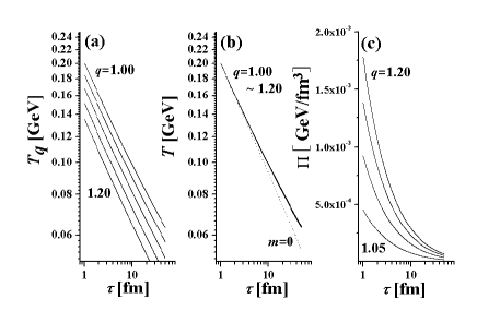
Figure 1: Proper time evolution of $T_{q}$, $T$ and $\Pi$ for $q$= 1.00-1.20. The $q$-hydrodynamical evolution starts at $\tau_{0}=1.0$ fm. The initial temperatures, $T_{q}(\tau_{0})$ are chosen in such way as to have $T_{0}=0.2$ GeV for all values of $q$. The doted line in (b) is obtained for a fluid composed of massless particles (in this case there is no $q$-dependence).

The $q$-hydrodynamical evolution starts at proper time $\tau_{0}=1.0$ fm with the $q$-temperature $T_{q}(\tau_{0})$ chosen such that $T_{0}\equiv T(\tau_{0})=0.2$ GeV. As seen in Fig. 1, although $T_{q}$ depends on $q$, the $T(\tau)$ does not (it scales with $q$). This is interesting because in the usual $d$-hydrodynamics cooling behavior (i.e., $T$) is affected by the viscous effects. However, in our case the $q$-dependence of Eq. (22) is only implicit and the corresponding EoS depends only very weakly on $q$ in the high temperature region (cf., Fig. 1 in OsadaPRC77 ). On the other hand, it depends on the mass of particles which composed our fluid. The bulk pressure $\Pi$ decreases monotonously with $\tau$ and increases with the non-extensive parameter $q$.

We close this example by discussing the corresponding Reynolds number BaymNPA418 ; KounoPRD41 . Separating in Eq. (22) dissipative and non-dissipative terms by using the Reynolds number $R_{e}$ MurongaPRC69 we get

$$\frac{d\varepsilon}{d\tau}+\frac{\varepsilon+P}{\tau}=\frac{(\varepsilon+P)}{\tau R_{e}},$$ (24)

In $q$-hydrodynamics with the NexDC conjecture

$${R_{e}}^{-1}=\frac{3\tau}{\varepsilon+P}\left(\frac{\Pi}{\tau}+\frac{d\Pi}{d\tau}\right).$$ (25)

Fig. 2 shows examples of proper time evolution of the inverse of Reynolds number obtained in Eq. (25). For comparison, the maximal values of $R_{e}^{-1}$ quoted in BaierPRC73 for $\tau_{0}=1$ fm and $T_{0}=0.3$ GeV are $R_{e}^{-1}\approx 0.065$ (for $\eta/s=0.08$ and at $\tau\approx 2$ fm) and $R_{e}^{-1}\approx 0.21$ (for $\eta/s=0.30$ and $\tau\approx 4$ fm). Our $R_{e}^{-1}$ remains smaller than these values, nevertheless we observe a similar maximum of $R_{e}^{-1}$ at finite proper time, $\tau\sim 10$ fm. Notice that one can rewrite Eq. (24) as $d\varepsilon/d\tau=(R^{-1}-1)w/\tau$, which, in the case of $R^{-1}>1$, may indicate the instability of our solution for large $\tau$ MurongaPRC69 . However, as one can see in Fig. 2, our $q$-hydrodynamical model with $q$-scaling solution gives very small values of $R_{e}^{-1}$, $R_{e}^{-1}\ll 1$. This, according to KounoPRD41 ; DenicolJPhysG35 , may guarantee the stability of the corresponding $d$-hydrodynamics obtained.

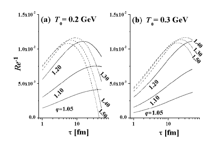
Figure 2: Proper time evolution of $R_{e}^{-1}$ obtained from $q$-hydrodynamics for two different initial temperatures (panels (a) and (b)) and for different values of the parameter $q$. Solid lines are for, respectively, $q=1.05$, $1.10$ and $1.20$, dashed lines are for $q=1.30-1.50$. The same EoS has been used as in Fig. 1.

To summarize: we have demonstrated that $d$-hydrodynamics obtained from the perfect $q$-hydrodynamics (by means of the NexDC conjecture) preserves its original causality. We believe then that $q$-hydrodynamics can serve as a phenomenological model of $d$-hydrodynamic with parameter $q$ describing summarily non ideality of the hadronic fluid. We have also shown that the corresponding inverse of the Reynolds number, $1/R_{e}$, may be small enough to ensure a stable hydrodynamical evolution of the corresponding strongly interacting quark/hadronic matter.

References

(1) T. Hirano, N. Kolk and A. Bilandzic, airXiv:0808.2684,
to appear in Springer Lecture Notes in Physics.
(2) T. D. Lee, Nucl. Phys. A750, 1 (2005).
(3) T. Hirano and M. Gyulassy, Nucl. Phys. A 769, 71 (2006).
(4) C. Eckart, Phys.Rev. 58, 919 (1940).
(5) W. A. Hiscock and L. Lindblom, Phys. Rev. D 31, 725 (1985); D 35, 3723
(1987).
(6) W. Israel, Ann. Phys. (N.Y.) 100, 310 (1976);
J. M. Stewart, Proc. R. Soc. London, Ser. A 357, 59 (1977);
W. Israel and J. M. Stewart, Ann Phys. (N.Y.) 118, 341 (1979).
(7) A. Muronga, Phys. Rev.C 69, 034903 (2004) and C 76, 014910 (2007).
(8) U. Heinz, H. Song and A.K. Chaudhuri, Phys. Rev. C 73, 034904 (2006);
H. Song and U. Heinz, Phys. Lett. B 658, 279 (2008).
(9) R. Baier and R. Romatschke and U. A. Wiedemann, Phys. Rev. C 73, 064903
(2006).
(10) T. Koide, G. S. Denicol, Ph. Mota and T. Kodama, Phys. Rev. C 75, 034909
(2007);
(11) A. K. Chaudhuri, Phys. Rev. C 74, 044904 (2006).
(12) P.Ván and T.S.Biro, Eur. Phys.J. Special Topics 155, 201
(2008); T.S. Biro, E. Molnar and P. Ván, Phys. Rev. C 78, 014909 (2008)
and references therein.
(13) T. Osada and G. Wilk, Phys. Rev. C 77, 044903 (2008) and
Prog. Theor. Phys. Suppl. 174, 168 (2008).
(14) C. Tsallis, J. Stat. Phys. 52 479 (1988).
For updated bibliography on this subject see
http://tsallis.cat.cbpf.br/ biblio.htm.
(15) A. Lavagno, Phys. Lett. A301, 13 (2002).
(16) J. A. S. Lima, R. Silva and A. R. Plastino, Phys. Rev. Lett. 86, 2983 (2001).
(17) T. Kodama, H. T. Elze, C. E. Aguiar and T. Koide, Europhys. Lett.
70, 439 (2005).
(18) T.S. Biró and G. Purcsel, Phys. Rev. Lett. 95 162302
(2005); Phys. Lett. A 372, 1174 (2008).
(19) T. Sherman and J. Rafelski, Lecture Notes in Physics 633 (2004) 377.
(20) J. D. Bjorken, Phys. Rev. D27, 140 (1983).
(21) G. Baym, Nucl. Phys. A418, 525c (1984).
(22) H.Kouno, M. Maruyama, F. Takagi, and K. Saito, Phys. Rev. D 41, 2903
(1990).
(23) G.S.Denicol, T. Kodama, T. Koide and Ph. Mota,
Phys. Rev. C 78, 034901 (2008).