Quantum Monte Carlo study of a magnetic-field-driven 2D superconductor-insulator transition

Abstract

We numerically study the superconductor-insulator phase transition in a model disordered 2D superconductor as a function of applied magnetic field. The calculation involves quantum Monte Carlo calculations of the $(2+1)$D $XY$ model in the presence of both disorder and magnetic field. The $XY$ coupling is assumed to have the form $-J\cos(\theta_{i}-\theta_{j}-A_{ij})$, where $A_{ij}$ has a mean of zero and a standard deviation $\Delta A_{ij}$. In a real system, such a model would be approximately realized by a 2D array of small Josephson-coupled grains with slight spatial disorder and a uniform applied magnetic field. The different values $\Delta A_{ij}$ then corresponds to an applied field such that the average number of flux quanta per plaquette has various integer values $N$: larger $N$ corresponds to larger $\Delta A_{ij}$. For any value of $\Delta A_{ij}$, there appears to be a critical coupling constant $K_{c}(\Delta A_{ij})=\sqrt{[J/(2U)]_{c}}$, where $U$ is the charging energy, above which the system is a Mott insulator; there is also a corresponding critical conductivity $\sigma^{*}(\Delta A_{ij})$ at the transition. For $\Delta A_{ij}=\infty$, the order parameter of the transition is a renormalized coupling constant $g$. Using a numerical technique appropriate for disordered systems, we show that the transition at this value of $\Delta A_{ij}$ takes place from an insulating (I) phase to a Bose glass (BG) phase, and that the dynamical critical exponent characterizing this transition is $z\sim 1.3$. By contrast, $z=1$ for this model at $\Delta A_{ij}=0$. We suggest that the superconductor to insulator transition is actually of this I to BG class at all nonzero $\Delta A_{ij}$’s, and we support this interpretation by both numerical evidence and an analytical argument based on the Harris criterion [A. B. Harris, J. Phys. C: Solid State Phys. 7, 1671 (1974)]. $K_{c}$ is found to be a monotonically increasing function of $\Delta A_{ij}$. For certain values of $K$, a disordered Josephson array may undergo a transition from an ordered, Bose glass phase to an insulator with increasing $\Delta A_{ij}$.

I INTRODUCTION

The superconductor-insulator (S-I) transition of thin two-dimensional (2D) superconducting films has been extensively studied both theoretically cha1 ; cha2 ; fisher89 ; krauth ; runge ; sorensen ; kampf ; batrouni93 ; makivic ; wallin ; hebert ; schmid ; lee1 ; lee2 ; nishiyama ; capriotti ; smakov and experimentally haviland ; samband ; markovic1 ; markovic2 ; yazdani for many years. The theoretical work can be broadly categorized into two groups: in one group, disorder is induced using a random chemical potential, while in the other, disorder is generated using a magnetic field. Most previous work belongs to the former cha1 ; krauth ; runge ; sorensen ; kampf ; batrouni93 ; makivic ; wallin ; lee1 ; lee2 ; smakov whereas only a few belong to the latter cha2 ; nishiyama ; markovic1 ; markovic2 .

The present work is motivated primarily by several experiments in which an S-I transition is observed in a 2D material as a function of applied transverse magnetic field. Such experiments have been reported in thin films of superconducting materials. They have also been carried out in some of the most anisotropic cuprate high-$T_{c}$ superconductors; in such materials, individual copper oxide layers may conceivably behave like thin superconducting films if they are well enough decoupled from the other layers hebard ; okuma95 ; goldman95 ; kapri ; okuma98 ; gantmakher00 ; markovic3 ; hao ; gantmakher03 ; baturina04 ; steiner1 ; baturina05 ; steiner2 ; aubin . In both cases, the films seem to undergo a transition from S to I with increasing magnetic field. Furthermore, the transition appears to be controlled mainly by the film resistance $R$. Experiments suggest that, in contrast to some predictions, $R$ does not have a universal value at the S-I transition gantmakher00 ; markovic3 . In view of these experiments, it seems useful to construct a simple model which contains disorder and also shows a field-driven transition. In the present paper we present such a model, and analyze its properties by a combination of numerical methods and scaling assumptions.

Before describing our own approach, we briefly review some of the previous theoretical work in this area. An early numerical calculation was carried out by Cha et al. cha1 at zero magnetic field ($B=0$). These workers calculated both analytically and numerically the zero-temperature ($T=0$) universal conductivity $\sigma^{*}$ of the 2D boson-Hubbard model without disorder at the S-I transition. They found, using numerical Monte Carlo (MC) simulations of a (2+1)D $XY$ model, that $\sigma^{*}=(0.285\pm 0.02)\sigma_{Q}$, where $\sigma_{Q}=(2e)^{2}/h$ is the quantum conductance. This result is close to the value obtained from an analytic large-$N$ expansion. They further studied this model under an applied transverse magnetic field using MC simulations, and found that $\sigma^{*}$ was increased cha2 .

Fisher et al. fisher89 studied the $T=0$ phase diagrams and phase transitions of bosons with short-range repulsive interactions moving in both periodic and random potentials. For the periodic case, they found the system exhibited two different phases, a superfluid and Mott insulator, and that the dynamic exponent $z$ exactly equaled the spatial dimension $d$. They also derived certain zero temperature constraints on the correlation length exponent $\nu$ and the order parameter correlation exponent $\eta$, namely $\nu\geq 2/d$ and $\eta\leq 2-d$. In the presence of disorder, they found that a “Bose glass” phase existed, and that the transition to a superfluid phase took place from the Bose glass phase, not directly from the Mott insulator.

Most previous studies in this area have been based on quantum Monte Carlo (QMC) simulations krauth ; runge ; sorensen ; batrouni93 ; makivic ; wallin ; hebert ; schmid ; lee1 ; lee2 ; capriotti . Some work has involved advanced QMC techniques, such as a QMC algorithm based on the exact duality transformation of the boson Hubbard model hebert , and a worm algorithm lee2 . Other studies have used a stochastic series expansion method hebert ; smakov and an exact diagonalization method nishiyama . Analytically, besides the large-$N$ expansion technique used in Ref. cha1 , a coarse-graining approximation kampf has been adopted in some investigations.

The numerical studies of the S-I transition have used a wide range of model Hamiltonians. Some workers have employed a 2D hard core boson model runge ; makivic ; hebert ; schmid ; nishiyama , while others used a 2D soft core boson Hamiltonian fisher89 ; batrouni90 ; krauth ; cha1 . This model has been used to investigate the S-I transition at $T=0$ sorensen ; kampf ; makivic ; nishiyama ; smakov ; samband , as well as the superconductor-Bose glass (S-BG) phase transition runge ; batrouni93 , while some workers have investigated both krauth ; wallin ; lee1 ; lee2 . In addition, Šmakov and Sørensen smakov studied the S-I transition at finite temperature $T$ using a similar model.

A number of workers have also investigated more complex phase transitions, of which we mention just a few representative examples. Capriotti et al. capriotti studied a reentrant superconducting-to-normal (S-N) phase transition using, as a model, a resistively shunted 2D Josephson junction array with normal Ohmic shunt resistors as the source of dissipation. Chakravarty et al. chakravarty also found a dissipation-induced phase transition in such an array, but did not study the possibility of reentrance. The reentrant S-N phase transition in Ref. capriotti was found to persist for moderate dissipation strength, but the superconducting phase was always found to be stabilized above a critical dissipation strength at sufficiently low $T$. Hébert et al. hebert studied phase transitions between superfluid, checkerboard, and striped solid order, using two interactions—a nearest-neighbor ($V_{1}$) and next-nearest-neighbor ($V_{2}$) repulsion—instead of a single parameter to describe the random chemical potential. They found that the model exhibited a superfluid to striped solid transition at half filling; away from half filling, they found a first-order transition from superfluid to striped supersolid, as well as a continuous transition from striped supersolid (superconducting) to striped solid (insulating). Schmid et al. schmid have studied a first order transition between a checkerboard solid and a superfluid phase at finite temperature. They also found that an unusual reentrant behavior in which ordering occurs with increasing temperature. As an effort to develop a more realistic model, several workers have included both short and long-range repulsive interactions between bosons sorensen ; wallin , and some studies have included fluctuations in the amplitude as well as the phase of the superconducting order parameter kampf .

The $T=0$ S-I transition has been found to be characterized by universal behavior. Ref. makivic found, using QMC, that the dynamic exponent, the correlation length exponent, and the universal conductivity were $z=0.5\pm 0.1$, $\nu=2.2\pm 0.2$, and $\sigma_{c}=(1.2\pm 0.2)\sigma_{Q}$, respectively. In the coarse-graining approximation kampf , the universal conductivity was found to be $\sigma^{*}=(\pi/8)\sigma_{Q}$, while the value $\sigma^{*}=(0.45\pm 0.05)\sigma_{Q}$ was obtained at finite $T$ using the stochastic series expansion with a geometric worm algorithm smakov ; in the latter work it was also found that $\sigma/\sigma_{Q}$ scaled with $\omega/T$ at small frequencies $\omega$ and low $T$. With only short-range Coulomb interactions, the universal conductivity at the phase transition was found to be $\sigma^{*}=(0.14\pm 0.03)\sigma_{Q}$ sorensen ; wallin . With long-range Coulomb interactions, this value increased to $\sigma^{*}=(0.55\pm 0.1)\sigma_{Q}$ sorensen or $\sigma^{*}=(0.55\pm 0.06)\sigma_{Q}$ wallin .

This critical behavior differs significantly from the $T=0$ S-BG transition. At this transition, the dynamical exponent and the universal conductivity were found to equal $z=1.95\pm 0.25$ and $\sigma^{*}=(0.17\pm 0.01)\sigma_{Q}$, respectively runge . Batrouni et al. batrouni93 found $\sigma^{*}=(0.45\pm 0.07)\sigma_{Q}$ from QMC calculations and $\sigma^{*}=(0.47\pm 0.08)\sigma_{Q}$ from analysis of current-current correlation functions.

At intermediate strength of disorder, Lee et al. lee1 found that the dynamical and the correlation length critical exponent were $1.35\pm 0.05$ and $\nu=0.67\pm 0.03$, respectively. They also found that a Mott insulator to superfluid transition occurred in the weak disorder regime while a Bose glass to superfluid transition took place in the strong disorder regime. More recently, Lee and Cha lee2 studied the quasiparticle energy gap near the quantum phase transition. They found that this gap vanished discontinuously at the transition for a weak disorder, implying a direct Mott insulator to superfluid transition, whereas this discontinuous jump disappeared for a strong disorder, supporting the intervention of Bose glass phase in this regime.

Several workers have studied the S-I transition by explicitly introducing a magnetic field, using various models and experiments. For example, Nishiyama nishiyama found that the 2D hard core boson model exhibited a field-tuned localization transition at a certain critical magnetic field and that the critical DC conductivity was substantially larger than that at zero magnetic field. In his work, the critical conductivity was found to be non-universal but instead increased with increasing magnetic field. Besides the experiments mentioned earlier, Sambandamurthy et al. samband found, from studies of thin amorphous InO films near the S-I transition, that the resistivity followed a power law dependence on the magnetic field in both the superconducting and the insulating phases.

In most of the above calculations, the QMC approach is based on a mapping between a $d$-dimensional quantum mechanical system and a $(d+1)$-dimensional classical system with the imaginary time as an extra dimension sondhi . This mapping works because calculating the thermodynamic variables of the quantum system is equivalent to calculating the transition amplitudes of the classical system when they evolve in the imaginary time. The imaginary time interval is fixed by the temperature of the system. The net transition amplitude between two states of the system can then be obtained by a summation over the amplitudes of all possible paths between them according to the prescription of Feynman feynman . These paths are the states of the system at each intermediate time step. Therefore, the path-integral description of the quantum system can be interpreted using the statistical mechanics of the $(d+1)$-dimensional classical system held at a fictitious temperature which measures zero-point fluctuations in the quantum system.

In order for a boson system to have a superconductor-insulator transition, the bosons must have an on-site repulsive interaction, i.e., a “charging energy.” Otherwise the boson system would usually undergo Bose-Einstein condensation at zero temperature. The charging energy induces zero-point fluctuations of the phases and disorders the system. On the other hand the Josephson or $XY$ coupling favors coherent ordering of the phases, which causes the onset of superconductivity. Therefore, the competition between the charging energy and $XY$ coupling is responsible for the superconductor-insulator transition, which typically occurs at a critical value of the ratio of the strengths of these two energies. In addition, if a disorder is added to the system, the system may also undergo a transition to a phase other than a Mott insulator, depending on the strength of the disorder. This additional phase is known to be a Bose glass phase.

In this work, we study the zero-temperature quantum phase transitions of 2D model superconducting films in an applied magnetic field. Our model includes both charging energy and Josephson coupling, and thus allows for an S-I transition. In our approach, the applied magnetic field is described by a root-mean-square (rms) fluctuation $\Delta A_{ij}$ which describes the randomness in the flux per plaquette. This randomness leads to the occurrence of a Bose glass phase at large $\Delta A_{ij}$. As explained further below, our model corresponds well to a 2D Josephson junction array with weak disorder in the plaquette areas, studied at an applied uniform magnetic field corresponding to integer number $N_{v}$, on average, of flux quanta per plaquette. The quantity $\Delta A_{ij}$ is proportional to the rms disorder in the flux per plaquette, and is proportional to $N_{v}$. Thus, our model gives rise to an S-I transition in the array with increasing $N_{v}$ (or increasing magnetic field).

The remainder of this paper is organized as follows. Sec. II presents the formalism. In this section, we give the model boson Hubbard model, and describe its conversion to a $(2+1)$D $XY$ model, which we treat using path-integral Monte Carlo calculations. We also describe the finite-size scaling methods for obtaining the critical coupling constants and universal conductivities at the transition. Finally, this section describes the nature of the renormalized coupling constant used to study the behavior of the system in the fully random case. Sec. III presents our numerical results, using these approaches. We discuss our results and present our conclusions in Sec. IV.

II FORMALISM

II.1 Model Hamiltonian

Our goal is to examine the superconductor-insulator transition in a disordered 2D system in a magnetic field at very low temperature $T$. Thus, a useful model for this transition would include three features: (i) a competition between a Coulomb energy and an energy describing the hopping of Cooper pairs; (ii) disorder; and (iii) a magnetic field. In particular, we hope that this model will exhibit, for suitable parameters, a transition from superconductor to insulator as the magnetic field is increased. While there are a wide range of models which could incorporate these features, we choose to consider a model Hamiltonian appropriate to a 2D Josephson junction array:

$${\cal H}^{\prime}=U\sum_{j}n_{j}^{2}-J\sum_{\langle ij\rangle}\cos(\theta_{i}-\theta_{j}-A_{ij}).$$ (1)

Here $n_{j}$ is the operator representing the number of Cooper pairs on a site $j$, $J$ is the Josephson energy coupling sites $i$ and $j$, $\theta_{i}$ is the phase of the order parameter on the $i$th site, $A_{ij}=(2\pi/\Phi_{0})\int_{i}^{j}{\bf A}\cdot d{\bf l}$ is a magnetic phase factor, $\Phi_{0}=hc/2e$ is the flux quantum, and ${\bf A}$ is the vector potential. In this picture, each site can be thought of as a superconducting grain.

For calculational convenience, we choose to take the sites $j$ to lie on a regular 2D lattice (a square lattice in our calculations), with Josephson coupling only between nearest neighbors. Thus, the disorder in our model is incorporated via the magnetic phase factors $A_{ij}$, as explained further below. Our Hamiltonian is identical to that of Cha et al. cha1 except that we consider the special case that the chemical potential $\mu_{i}$ for Cooper pairs on the $i$th grain is an integer, and we choose the $A_{ij}$’s to be random.

The first term in Eq. (1) is the charging energy. We consider only a diagonal charging energy and also assume all grains to be of the same size, so that $U$ is independent of $j$. Since the charging energy $E_{Cj}$ of a grain carrying charge $Q_{j}$ with capacitance $C$ is $E_{Cj}=Q_{j}^{2}/(2C)$,

$$U=\frac{(2e)^{2}}{2C}=\frac{2e^{2}}{C}.$$ (2)

We also know that $Q_{j}=CV_{j}$, where $V_{j}$ is the voltage of grain $j$ relative to ground; so

$$E_{Cj}=\frac{1}{2}CV_{j}^{2}=\frac{C\hbar^{2}}{2(2e)^{2}}\dot{\theta}_{j}^{2},$$ (3)

where we have used the Josephson relation, $V_{j}=(\hbar/2e)\dot{\theta}_{j}$. Finally, we can express $C$ in terms of $U$ using Eq. (2), with the result

$$E_{Cj}=\frac{\hbar^{2}}{4U}\dot{\theta}_{j}^{2}.$$ (4)

Combining all these relations, we obtain

$${\cal H}^{\prime}=\frac{\hbar^{2}}{4U}\sum_{j}\dot{\theta}_{j}^{2}-J\sum_{\langle ij\rangle}\cos(\theta_{i}-\theta_{j}-A_{ij}).$$ (5)

Since we have taken the grains to lie on a lattice, we need to choose the $A_{ij}$’s in a way which incorporates randomness. Thus, we make the simplifying assumption that the phase factor $A_{ij}$ of each bond in the plane is an independent Gaussian random variable with a mean of zero and a standard deviation $\Delta A_{ij}$:

$$P(A_{ij})=\frac{1}{\sqrt{2\pi}(\Delta A_{ij})}\exp\left[-\frac{A_{ij}^{2}}{2(\Delta A_{ij})^{2}}\right].$$ (6)

Since the sum of the phase factors around the four bonds of a plaquette is $2\pi/\Phi_{0}$ times the flux through that plaquette, this choice will cause the flux through the plaquette also to be a random variable. However, the fluxes through nearest-neighbor plaquettes will be correlated.

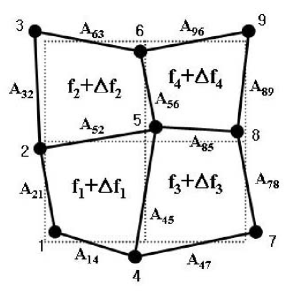
Although this model may seem artificial, it should closely resemble a real, physically achievable system. Specifically, consider a spatially random distribution of grains in 2D in a uniform magnetic field. Suppose that the grain positions deviate slightly (but randomly) from the sites of a square lattice. Then the areas of the square plaquettes have a random distribution, and consequently, the flux through each plaquette also varies randomly about its mean. If the average flux $\Phi$ per plaquette is $\Phi=f\Phi_{0}$, then the root-mean-square deviation of the flux, $\Delta\Phi\propto f$ as in Fig. 1.

Figure 1: Sketch of a $2\times 2$ group of plaquettes in a square lattice of Josephson-coupled grains, in which each grain is randomly displaced by a small amount from its nominal lattice site. In a uniform transverse magnetic field, if the average flux $\Phi$ per plaquette is $\Phi=f\Phi_{0}$, then the root-mean-square deviation of the flux from its mean value is also proportional to $f$.

Now consider the special case of integer $f$. In the absence of disorder, the 2D array at integer $f$ should behave exactly like the array at $f=0$, because the Hamiltonian would then be perfectly periodic in $f$ shih1 ; shih2 ; shih3 . With nonzero disorder, only the rms deviation from integer $f$, i.e., $\Delta f=\Delta\Phi/\Phi_{0}$, is physically relevant. This deviation increases linearly with $f$.

In short, our model Hamiltonian is approximately realized by a 2D Josephson junction array on a square lattice, in which the grains deviate randomly in position from their lattice sites, placed in a transverse magnetic field with an average flux per plaquette $f\Phi_{0}$, with integer $f$. A larger $\Delta A_{ij}$ corresponds to a larger $f$. The models are not equivalent, even if the random position deviations are specified by Gaussian variables, because we assume the $\Delta A_{ij}$’s for different bonds are uncorrelated, whereas they would be correlated in the positionally disordered case. However, this difference should have little effect in practice and we have confirmed this in the limit of large $f$ (see below). For non-integer $f$, the disordered 2D Josephson array has well-known oscillatory properties as a function of $f$ which are not described by our model as formulated above. This disordered Josephson array is not an entirely realistic model of a superconducting film which undergoes a field-driven superconductor-insulator transition because our model involves an underlying lattice of grains. Nonetheless, we may hope that some of the properties of our model resemble those seen in experimentally studied materials.

A related method of including random flux has previously been used by Huse and Seung huse as a model for a three-dimensional (3D) “gauge glass.” These workers considered only $\Delta A_{ij}=\infty$, and studied a 3D classical model (U = 0) rather than the 2D quantum case considered here.

II.2 Path Integral Formulation

We can now use the model Hamiltonian (5) to obtain the action in the form of a standard integral over imaginary time. The action $S$ may be written

$$\frac{S}{\hbar}=\frac{1}{\hbar}\int{\cal L}d\tau,$$ (7)

where ${\cal L}$ is the Lagrangian, given by

$${\cal L}=\frac{\hbar^{2}}{4U}\sum_{j}\left(\frac{\partial\theta_{j}}{\partial\tau}\right)^{2}-J\sum_{\langle ij\rangle}\cos[\theta_{i}(\tau)-\theta_{j}(\tau)-A_{ij}(\tau)].$$ (8)

The partition function is now given by a path integral of $\exp(-S/\hbar)$ over all possible paths described by the variables $\theta_{i}(\tau)$ in imaginary time $\tau$, integrated from $\tau=0$ to $\tau=\beta\hbar$, where $\beta=1/(k_{B}T)$. This path integral can be reduced to the partition function of an anisotropic classical $XY$ model in three dimensions. Here, by “anisotropic” we mean that the coupling constants $K$ and $K_{\tau}$ in the $xy$ plane and $\tau$ direction are different. To make the mapping, we first write

$$\left(\frac{\partial\theta_{i}}{\partial\tau}\right)^{2}\sim\left(\frac{\Delta\theta_{i}}{\Delta\tau}\right)^{2}\sim\frac{2-2\cos\Delta\theta_{i}}{(\Delta\tau)^{2}},$$ (9)

where $\Delta\tau$ is the width of the time slice, $\Delta\theta_{i}=\theta_{i}(\tau+\Delta\tau)-\theta_{i}(\tau)$, and we have used the expansion of $\cos\Delta\theta$ to second order in the small quantity $\Delta\theta$. This expansion is accurate when $\Delta\tau$ is sufficiently small.

Neglecting the constant term in this expansion, we finally obtain

$$\frac{S}{\hbar} = -K_{\tau}\sum\cos[\theta_{i}(\tau)-\theta_{i}(\tau+\Delta\tau)]$$ (10)

$$-K\sum\cos[\theta_{i}(\tau)-\theta_{j}(\tau)-A_{ij}(\tau)].$$

Here the sums run over all bonds in the $\tau$ direction and in the $xy$ plane, respectively.

In order to obtain the values of the coupling constants $K$ and $K_{\tau}$, we assume that we have broken up the time integral into $M$ time slices, each of width $\beta\hbar/M$. Then the coupling constant in the $xy$ direction is just

$$K=\frac{\beta J}{M}.$$ (11)

The coupling constant in the $\tau$ direction is given by

$$K_{\tau}=\frac{\hbar^{2}}{4U}\frac{1}{\hbar}(\Delta\tau)\frac{2}{(\Delta\tau)^{2}}=\frac{1}{2U}\frac{\hbar}{\Delta\tau}=\frac{M}{2\beta U},$$ (12)

we have used $\Delta\tau=\beta\hbar/M$ and included the extra factor of $2$ in the numerator because $\cos\Delta\theta\sim 1-(\Delta\theta)^{2}/2$.

Given $K$ and $K_{\tau}$, the partition function is obtained from this anisotropic 3D $XY$ classical Hamiltonian with coupling constants $K$ and $K_{\tau}$. Any desired equilibrium quantity can, in principle, be computed by averaging over all configurations using standard classical Monte Carlo techniques. Within any given realization of the disorder, the $A_{ij}$’s are chosen at random from the Gaussian distribution within the $xy$ plane, as described above, but the $A_{ij}$’s for a given bond in the $xy$ plane are independent of $\tau$, i.e., they are the same for all time slices. In principle, for any given $\beta$, this should be done taking the limit as $M\rightarrow\infty$. In practice, of course, the size of the sample is limited by considerations of computer time.

II.3 Evaluation of Specific Properties Using Path Integral Formulation

The time-slice formulation of the partition function allows various properties to be evaluated using standard classical Monte Carlo techniques. We now review how this may be done for the helicity modulus (or superfluid density) and the electrical conductivity. Similar formulations have been given in Refs. fisher73 ; ohta ; shih2 ; shih3 ; cha1 ; cha2 for different but related models.

II.3.1 Helicity Modulus

For a frustrated classical $XY$ system in $d$ dimensions, the helicity modulus tensor $\gamma_{\alpha\beta}$ is a $d\times d$ matrix which is a measure of the phase stiffness. It is defined as the second derivative of the free energy with respect to an infinitesimal phase twist, and may be written

$$\gamma_{\alpha\beta}=\frac{1}{N}\left.\frac{\partial^{2}F}{\partial A_{\alpha}^{\prime}\partial A_{\beta}^{\prime}}\right|_{{\bf A}^{\prime}=0},$$ (13)

where $N$ is the number of sites in the system and ${\bf A}^{\prime}$ is a fictitious vector potential added to the Hamiltonian (in addition to the vector potential ${\bf A}$ already included in the Hamiltonian fisher73 ). In explicit form, this derivative takes the following form for the diagonal elements (see, e.g., Ref. kim ):

$$\gamma_{\alpha\alpha}=\frac{1}{N}\left\langle\sum_{\langle ij\rangle}J_{ij}\cos(\theta_{i}-\theta_{j}-A_{ij})(\hat{e}_{ij}\cdot\hat{e}_{\alpha})^{2}\right\rangle$$

$$-\frac{1}{Nk_{B}T}\left\langle\left[\sum_{\langle ij\rangle}J_{ij}\sin(\theta_{i}-\theta_{j}-A_{ij})(\hat{e}_{ij}\cdot\hat{e}_{\alpha})\right]^{2}\right\rangle$$

$$+\frac{1}{Nk_{B}T}\left\langle\sum_{\langle ij\rangle}J_{ij}\sin(\theta_{i}-\theta_{j}-A_{ij})(\hat{e}_{ij}\cdot\hat{e}_{\alpha})\right\rangle^{2}.$$ (14)

Here $\hat{e}_{ij}$ is a unit vector from the $i$th to the $j$th site, and $\hat{e}_{\alpha}$ is a unit vector in the $\alpha$ direction. The triangular brackets denote an average in the canonical ensemble.

If this expression is applied to the time-slice representation of the quantum-mechanical Hamiltonian, the coupling constants $J_{ij}$ will be different in the $xy$ plane and in the $\tau$ direction. For the time-slice calculation, we have to be careful in order to obtain a result which is well-behaved in the limit $M\rightarrow\infty$, where $M$ is the number of time slices. The correct expression in this case is

$$\gamma_{xx}=\frac{1}{N_{x}N_{y}}\left\langle\frac{J}{M}\sum_{\langle ij\rangle\|\hat{x}}\cos(\theta_{i}-\theta_{j}-A_{ij})\right\rangle$$

$$-\frac{1}{N_{x}N_{y}k_{B}T}\left\langle\left[\sum_{\langle ij\rangle\|\hat{x}}\frac{J}{M}\sin(\theta_{i}-\theta_{j}-A_{ij})\right]^{2}\right\rangle$$

$$+\frac{1}{N_{x}N_{y}k_{B}T}\left\langle\sum_{\langle ij\rangle\|\hat{x}}\frac{J}{M}\sin(\theta_{i}-\theta_{j}-A_{ij})\right\rangle^{2}.$$ (15)

Here we are assuming that there are $N_{x}N_{y}$ superconducting grains in our 2D lattice and $M$ time slices. The sums run over all distinct bonds in the $\hat{x}$ direction; there are $N_{x}N_{y}M$ of these bonds ($N_{x}N_{y}$ per time slice). A similar expression holds for $\gamma_{yy}$. The in-plane coupling constant is taken to be $J/M$ because there are $M$ time slices.

From the above form, we can see why the expression behaves correctly in the limit $M\rightarrow\infty$. Each of the two sums contains $N_{x}N_{y}M$ terms in it, but the ensemble average consists of $M$ identical terms, one for each layer. Therefore, the first sum in Eq. (15), for example, should take the form

$$\frac{J}{M}\left\langle\sum_{\langle ij\rangle}\cos(\theta_{i}-\theta_{j}-A_{ij})\right\rangle$$

$$\longrightarrow J\left\langle\sum^{\prime}_{\langle ij\rangle}\cos(\theta_{i}-\theta_{j}-A_{ij})\right\rangle,$$ (16)

where the sum on the right hand side runs only over the phases in a single layer. The right-hand side is evidently independent of $M$ in the limit $M\rightarrow\infty$. A similar argument can be used to show that the second part of the expression (15) for $\gamma_{xx}$ also approaches a well-behaved limit as $M\rightarrow\infty$. Our numerical results confirm this behavior.

As an illustration, we write down an expression for $\gamma_{xx}$ in the limit $T\rightarrow 0$ in the unfrustrated case ($\Delta A_{ij}=0$). First, we multiply expression (15) by $\beta/M$ to obtain

$$\frac{\beta\gamma_{xx}}{M}=\frac{1}{N_{x}N_{y}M}\left\langle K\sum_{\langle ij\rangle\|\hat{x}}\cos(\theta_{i}-\theta_{j}-A_{ij})\right\rangle$$

$$-\frac{1}{N_{x}N_{y}M}\left\langle\left[\sum_{\langle ij\rangle\|\hat{x}}K\sin(\theta_{i}-\theta_{j}-A_{ij})\right]^{2}\right\rangle$$

$$+\frac{1}{N_{x}N_{y}M}\left\langle\sum_{\langle ij\rangle\|\hat{x}}K\sin(\theta_{i}-\theta_{j}-A_{ij})\right\rangle^{2},$$ (17)

where $K=\beta J/M$. The corresponding coupling constant in the $\tau$ direction is $K_{\tau}=M/(2\beta U)$.

Since we are interested in the limit $\beta\gg 1$, we choose $M$ so that $K=K_{\tau}$. This condition is equivalent to

$$\frac{\beta}{M}=\frac{1}{\sqrt{2JU}}.$$ (18)

Hence, we get

$$\frac{\gamma_{xx}}{\sqrt{2JU}}=\frac{1}{N_{x}N_{y}M}\left\langle K\sum_{\langle ij\rangle\|\hat{x}}\cos(\theta_{i}-\theta_{j}-A_{ij})\right\rangle$$

$$-\frac{1}{N_{x}N_{y}M}\left\langle\left[\sum_{\langle ij\rangle\|\hat{x}}K\sin(\theta_{i}-\theta_{j}-A_{ij})\right]^{2}\right\rangle$$

$$+\frac{1}{N_{x}N_{y}M}\left\langle\sum_{\langle ij\rangle\|\hat{x}}K\sin(\theta_{i}-\theta_{j}-A_{ij})\right\rangle^{2},$$ (19)

where $K=\beta J/M=\sqrt{J/(2U)}$. Since $K=K_{\tau}$, the right-hand side of this equation represents a dimensionless helicity modulus $\tilde{\gamma}$ for a classical unfrustrated isotropic 3D $XY$ model on a simple cubic lattice, which is a function of a single dimensionless coupling constant $K$.

Now it is known from previous Monte Carlo studies li ; gottlob ; fernandez ; schultka ; ryu that the unfrustrated 3D $XY$ model on a simple cubic lattice has an ordered phase if $K>K_{c}\sim 1/2.21\sim 0.452$. Therefore, $\tilde{\gamma}(K)$ vanishes if $K<K_{c}$ and is positive for $K>K_{c}$. Translating this result to the 2D quantum $XY$ model on a square lattice, we see that there is a superconductor-insulator transition at $J/(2U)=(0.452)^{2}=0.204$.

For reference we give the connection between our formulation of the helicity modulus and the calculation of Cha et al. cha1 Rather than the helicity modulus, these workers calculate the quantity $\rho(0)$, which is related to the superfluid density $\rho_{s}$ by

$$\rho(0)=\frac{\rho_{s}}{k_{B}T}$$ (20)

and to the components of the helicity modulus tensor by $\rho(0)=K\gamma\equiv K(\gamma_{xx}+\gamma_{yy})/2$, where $\gamma_{xx}=\gamma_{yy}$ for the present model, which is isotropic in the $xy$ plane. In our notation, $\rho(0)$ is given by

$$\rho(0) = \frac{JK}{2N_{x}N_{y}M}\left[\left\langle\sum_{\langle ij\rangle\|\hat{x}}\cos(\theta_{i}-\theta_{j}-A_{ij})\right\rangle\right.$$ (21)

$$\left.+\left\langle\sum_{\langle ij\rangle\|\hat{y}}\cos(\theta_{i}-\theta_{j}-A_{ij})\right\rangle\right]$$

$$-\frac{JK^{2}}{2N_{x}N_{y}M}\left[\left\langle\left[\sum_{\langle ij\rangle\|\hat{x}}\sin(\theta_{i}-\theta_{j}-A_{ij})\right]^{2}\right\rangle\right.$$

$$\left.+\left\langle\left[\sum_{\langle ij\rangle\|\hat{y}}\sin(\theta_{i}-\theta_{j}-A_{ij})\right]^{2}\right\rangle\right]$$

$$+\frac{JK^{2}}{2N_{x}N_{y}M}\left[\left\langle\sum_{\langle ij\rangle\|\hat{x}}\sin(\theta_{i}-\theta_{j}-A_{ij})\right\rangle^{2}\right.$$

$$\left.+\left\langle\sum_{\langle ij\rangle\|\hat{y}}\sin(\theta_{i}-\theta_{j}-A_{ij})\right\rangle^{2}\right].$$

II.3.2 Specific Heat

For the specific heat $C_{V}$, we used the fluctuation-dissipation theorem given by

$$C_{V}=\frac{\langle\mathcal{H}^{\prime 2}\rangle-\langle\mathcal{H}^{\prime}\rangle^{2}}{Nk_{B}T^{2}},$$ (22)

where $N$ is the total number of sites in the lattice, $\mathcal{H}^{\prime}$ is the Hamiltonian in Eq. (5), and $\langle\cdots\rangle$ denotes an ensemble average.

II.3.3 Conductivity

The conductivity in the low-frequency limit can also be obtained from the time-slice Monte Carlo approach as cha1

$$\sigma(0)=2\pi\sigma_{Q}\lim\limits_{k\to 0}\frac{\rho(k)}{k},$$ (23)

where $\rho(k)$ is proportional to the superfluid density at frequency $k$ and is given by

$$\rho(k) = \frac{JK}{2N_{x}N_{y}M}\left[\left\langle\sum_{\langle ij\rangle\|\hat{x}}\cos(\theta_{i}-\theta_{j}-A_{ij})\right\rangle\right.$$ (24)

$$\left.+\left\langle\sum_{\langle ij\rangle\|\hat{y}}\cos(\theta_{i}-\theta_{j}-A_{ij})\right\rangle\right]$$

$$-\frac{JK^{2}}{2N_{x}N_{y}M}\left\langle\sum_{\langle ij\rangle\|\hat{x},{\bf x}}\sin(\theta_{i}-\theta_{j}-A_{ij})e^{-i{\bf k}\cdot{\bf x}}\right.$$

$$\left.\times\sum_{\langle ij\rangle\|\hat{x},{\bf x}}\sin(\theta_{i}-\theta_{j}-A_{ij})e^{i{\bf k}\cdot{\bf x}}\right\rangle$$

$$-\frac{JK^{2}}{2N_{x}N_{y}M}\left\langle\sum_{\langle ij\rangle\|\hat{y},{\bf x}}\sin(\theta_{i}-\theta_{j}-A_{ij})e^{-i{\bf k}\cdot{\bf x}}\right.$$

$$\left.\times\sum_{\langle ij\rangle\|\hat{y},{\bf x}}\sin(\theta_{i}-\theta_{j}-A_{ij})e^{i{\bf k}\cdot{\bf x}}\right\rangle$$

$$+\frac{JK^{2}}{2N_{x}N_{y}M}\left\langle\sum_{\langle ij\rangle\|\hat{x},{\bf x}}\sin(\theta_{i}-\theta_{j}-A_{ij})e^{-i{\bf k}\cdot{\bf x}}\right\rangle$$

$$\times\left\langle\sum_{\langle ij\rangle\|\hat{x},{\bf x}}\sin(\theta_{i}-\theta_{j}-A_{ij})e^{i{\bf k}\cdot{\bf x}}\right\rangle$$

$$+\frac{JK^{2}}{2N_{x}N_{y}M}\left\langle\sum_{\langle ij\rangle\|\hat{y},{\bf x}}\sin(\theta_{i}-\theta_{j}-A_{ij})e^{-i{\bf k}\cdot{\bf x}}\right\rangle$$

$$\times\left\langle\sum_{\langle ij\rangle\|\hat{y},{\bf x}}\sin(\theta_{i}-\theta_{j}-A_{ij})e^{i{\bf k}\cdot{\bf x}}\right\rangle.$$

In the limit of very small $k$, we expect that $\rho(k)$ will remain finite in the superconducting phase and vanish in the insulating phase. Thus, $\sigma(0)$ will become infinite in the superconducting phase but vanish in the insulating phase. Precisely at the critical value $K_{c}$, $\sigma(0)$ will become finite with a universal value, as already obtained by other workers for related models.

III Quantum Monte Carlo Results

III.1 Numerical Procedure

In our quantum Monte Carlo calculations, we use the standard Metropolis algorithm with periodic boundary conditions in both the spatial directions and the imaginary time direction. We usually start with a random configuration of phases at $K=0.4$, then increase $K$ up to $K=0.7$ in steps of $0.005$. This procedure corresponds to lowering the temperature $T$ since $K\propto 1/T$. At each $K$, we take 40000 MC steps per site through the entire lattice to equilibrate the system, after which we take an additional 50000 MC steps to calculate the thermodynamic variables of interest. For a lattice size of $6^{3}$, we use ten times as many MC steps as these for both equilibration and averaging, and for a lattice size of $8^{3}$, we use twice as many steps.

For the phases $\theta_{i}$ of the order parameter on each site, we use the $360$-state clock model instead of a continuous angle between $0$ and $2\pi$ since it allows us to cover the entire range of angles with fewer trials. Therefore, the allowable angles are $0^{\circ}$, $1^{\circ}$, $2^{\circ}$,…, $359^{\circ}$. It has been shown numerically that these discrete phase angles give results indistinguishable from the continuous ones provided that $n>20$ thijssen . However, we select $A_{ij}$ from a continuous distribution in all our calculations.

For the partially random and completely random $A_{ij}$, we averaged over 100 different realizations of $\Delta A_{ij}$ to calculate the helicity modulus $\gamma$ and the specific heat $C_{V}$. These calculations were so time-consuming that we could go just up to $20\times 20\times 20$ lattice size. For this reason, we chose to carry out simulations only over four different $\Delta A_{ij}$ for the partially random case: $\Delta A_{ij}=1/2$, $1/\sqrt{2}$, $(1+1/\sqrt{2})/2\approx 0.854$, and $1$. Each realization is specified by a different random number seed.

III.2 Finite-Size Scaling for $\gamma(0)$

In general, if there is a continuous phase transition as a function of some parameter, such as the coupling constant $K$, the critical behavior near the transition can be analyzed by carrying out a finite-size scaling analysis of various calculated quantities. For example, the zero-frequency helicity modulus $\gamma(0)$ is expected to satisfy wallin

$$\gamma(0)=\frac{1}{L^{d+z-2}}\tilde{\gamma}\left(L^{1/\nu}\delta,\frac{L_{\tau}}{L^{z}}\right),$$ (25)

where $d$ is the spatial dimensionality, $z$ is the dynamic exponent, $\tilde{\gamma}$ is a scaling function, $\nu$ is the critical exponent for the correlation length $\xi$, $\delta=(K-K_{c})/K_{c}$, $K_{c}$ is the critical value of the coupling constant, and $L_{\tau}$ is the thickness in the imaginary time direction. For our present system, $d=2$, so the right-hand side is $L^{-z}\tilde{\gamma}(L^{1/\nu}\delta,L_{\tau}/L^{z})$. If we define $\tilde{\gamma}(L^{1/\nu}\delta,L_{\tau}/L^{z})=(L^{z}/L_{\tau})\tilde{G}(L^{1/\nu}\delta,L_{\tau}/L^{z})$, then this scaling relation becomes

$$L_{\tau}\gamma(0)=\tilde{G}\left(L^{1/\nu}\delta,\frac{L_{\tau}}{L^{z}}\right).$$ (26)

If our computational box has $N_{x}\times N_{y}\times M$ sites, with $N_{x}=N_{y}$, this scaling relation may be equivalently written as

$$KM\gamma(0)=\tilde{G}\left(N_{x}^{1/\nu}\delta,\frac{M}{N_{x}^{z}}\right).$$ (27)

As has been noted by other workers cha1 ; sorensen ; cha2 ; wallin ; lee1 ; hlee ; fabien ; hitchcock , $K_{c}$ can now be found, if $\gamma$ is a suitable order parameter, by plotting $KM\gamma(0)$ as a function of $\delta$ for various cell sizes, all with aspect ratios satisfying $M=cN_{x}^{z}$, and finding the point where these all cross, which corresponds to $\delta=0$. Unfortunately, this method requires knowing the value of $z$ in advance. For many such quantum phase transitions, $z$ may not be known. Thus, one should carry out this calculation for all plausible values of $z$ and find out which value leads to a satisfactory crossing. This procedure is prohibitively demanding numerically. We have, therefore, initially attempted to carry out scaling using $z=1$, the value which is known to be correct at $\Delta A_{ij}=0$. If this value were correct also at $\Delta A_{ij}\neq 0$, it would suggest that the superconducting-insulating transition at finite $\Delta A_{ij}$ is in the same universality class as the zero-field transition. In practice, we find that $z=1$ never gives perfect scaling at nonzero $\Delta A_{ij}$ and the scaling fit becomes progressively worse as $\Delta A_{ij}$ increases. For large $\Delta A_{ij}$ in particular, the fit clearly fails, and we find for these values that $\gamma(0)$ never converges to a nonzero value. At such large $\Delta A_{ij}$, we suggest that this regime corresponds to a Bose glass (as further discussed below), and carry out a different kind of scaling calculation to obtain the actual value of $z$ of this phase at $\Delta A_{ij}=\infty$. We also give arguments suggesting that, in fact, this Bose glass phase is actually the ordered phase for all nonzero values of $\Delta A_{ij}$.

Operationally, we implement the hypothesis that $z=1$ by taking $N_{x}=N_{y}=M$. With this choice, Eq. (27) becomes

$$KM\gamma(0)=\tilde{G}(M^{1/\nu}\delta,1)$$ (28)

when $d=2$.

III.3 Zero Magnetic Field

As a check of our method, we have calculated $K_{c}$ for the case of zero magnetic field ($A_{ij}=0$), using the above numerical approach. When there is no magnetic field, we get $K_{c}=0.4543\pm 0.0011$ using a finite-size scaling analysis of the helicity modulus $\gamma$ as shown in Fig. 2. This value is very close to $K_{c}=0.4539\pm 0.0013$ by the series expansion as in Ref. ferer , which is also used in Ref. cha1 . This result confirms the validity of our numerical codes. Using our value of $K_{c}$, we can also obtain the universal conductivity $\sigma^{*}/\sigma_{Q}=0.282\pm 0.005$. This result is also very close to the value $\sigma^{*}/\sigma_{Q}=0.285\pm 0.02$, obtained in Ref. cha1 .

Figure 2: Plot of $\gamma L_{\tau}$ as a function of $K$ for various $N_{x}\times N_{y}\times M$ lattices for $A_{ij}=0$. In this and all subsequent figures, unless otherwise specified, we use $N_{x}=N_{y}=M$. The phase transition occurs where the curves of different $M$ cross. The crossing point yields $K_{c}=0.4543\pm 0.0011$. The use of $N_{x}=N_{y}=M$ is equivalent to assuming that the dynamic exponent $z=1$, as discussed in the text.

III.4 Finite $\Delta A_{ij}$

Figs. 3(a), 3(b), and 4 show the helicity modulus $\gamma$, the specific heat $C_{V}$, and the finite-size scaling behavior of $\gamma$ as a function of coupling constant $K$ for several lattice sizes when $\Delta A_{ij}=1/2$. When $K>0.55$, $\gamma$ and $C_{V}$ appear to be nearly lattice size independent. The error bars from the jackknife method newman1 are shown in Fig. 3(a), but they are smaller than the symbol sizes. The lines are cubic spline fits to the data in Fig. 3(b). The apparent crossing point in Fig. 4 yields the critical coupling constant $K_{c}=0.491\pm 0.001$, which is very close to the peak of $C_{V}$ in Fig. 3(b).

Figure 3: (a) Helicity modulus $\gamma$ and (b) specific heat $C_{V}$, plotted as functions of coupling constant $K$ for several lattice sizes when $\Delta A_{ij}=1/2$. The error bars in (a), as obtained from the jackknife method, are smaller than the symbol sizes. The lines in (b) are cubic spline fits to the Monte Carlo data.

Figure 4: Finite-size scaling behavior of the data in Fig. 3(a), using $z=1$. The apparent crossing point yields $K_{c}=0.491\pm 0.001$.

The corresponding results for $\Delta A_{ij}=1/\sqrt{2}$ are shown in Figs. 5(a), 5(b), and 6. Compared to Fig. 3(a), $\gamma$ shows more lattice size dependence when $K>K_{c}$ in Fig. 5(a). The apparent crossing point in Fig. 6 yields $K_{c}=0.533\pm 0.001$. This $K_{c}$ is also very close to the peak in $C_{V}$ as in Fig. 5(b).

Figure 5: Same as Fig. 3, except that $\Delta A_{ij}=1/\sqrt{2}$.

Figure 6: Same as Fig. 4, except that the data are from Fig. 5(a). The apparent crossing point yields $K_{c}=0.533\pm 0.001$, as indicated by the vertical dashed line.

The results for $\gamma$, $C_{V}$, and $\gamma L_{\tau}$ when $\Delta A_{ij}=0.854$ are shown in Figs. 7(a), 7(b), and 8. In this case, the lattice size-dependence of $\gamma$ when $K>K_{c}$ in Fig. 7(a) becomes more conspicuous than that of Fig. 5(a). The apparent crossing point for the different sizes in Fig. 8 is less clearly defined than in the previous examples, but yields $K_{c}=0.585\pm 0.004$. This $K_{c}$ is slightly larger than the value of $K$ at the maximum of the broad peak in $C_{V}$, as in Fig. 7(b). There are some fluctuations of $\gamma L_{\tau}$ around $K=0.70$ for the lattice size of $12^{3}$ and larger fluctuations above $K_{c}$ for the lattice sizes of $16^{3}$ and $20^{3}$ in Fig. 8.

Figure 7: Same as Fig. 3, except that $\Delta A_{ij}=0.854$.

Figure 8: Same as Fig. 4, except that the data are from Fig. 7(a). The apparent crossing point yields $K_{c}=0.585\pm 0.004$.

The fact that the apparent crossing point in Fig. 8 is even less clear than those for smaller values of $\Delta A_{ij}$ suggests that $z\neq 1$. We present a more likely scenario for this and other values of $\Delta A_{ij}$ in the discussion section below.

As a final calculation for partially random $A_{ij}$, we use $\Delta A_{ij}=1.0$. The corresponding three thermodynamic variables $\gamma$, $C_{V}$, and $\gamma L_{\tau}$ are shown in Figs. 9(a), 9(b), and 10, respectively. The lattice size-dependence of $\gamma$ in Fig. 9(a) becomes far more conspicuous than the previous two examples. The peak of $C_{V}$ is very broad, as shown in Fig. 9(b). In addition, there is nothing like a clear crossing point of $\gamma L_{\tau}$ for different sizes $N_{x}$ in Fig. 10. We interpret this result to mean that the helicity modulus $\gamma$ does not play the role of an order parameter and that the transition is not a superconductor-to-insulator transition of the same character as at $\Delta A_{ij}=0$. Furthermore, there are strong fluctuations of $\gamma L_{\tau}$ as a function of $N_{x}$ when $K\geq 0.64$ for most lattice sizes, as can be seen in Fig. 10. We believe that, for this value (and, in fact, at all nonzero values) of $\Delta A_{ij}$, this is a transition from a Bose glass to a Mott insulator.

Figure 9: Same as Fig. 3, except that $\Delta A_{ij}=1.0$.

Figure 10: Same as Fig. 4, except that the data are from Fig. 9(a). In this case, the plots of $L_{\tau}\gamma(K)$ for different $N_{x}$ do not cross, suggesting that the helicity modulus $\gamma$ is no longer a suitable order parameter at $\Delta A_{ij}=1.0$.

Finally, we have considered the case of a fully random $A_{ij}$, $\Delta A_{ij}=\infty$. We implemented this by choosing $\Delta A_{ij}$ randomly between $0$ and $2\pi$. The helicity modulus $\gamma$ and the specific heat $C_{V}$ for this case are shown in Figs. 11(a) and 12(a), respectively. The magnitude of $\gamma$ becomes much smaller than those of previous cases, so that the error bars are easily visible on the scale of the plot. The helicity modulus even seems to have negative values for certain values of $K$, depending on the lattice size. Such negative values and fluctuations of the helicity modulus in a disordered superconductor were already reported in other work spivak , in the context of a different model. As in Figs. 9(a) and 10, $\gamma$ is strongly lattice-size dependent and there exists no value of $K$ at which the curves of $L_{\tau}\gamma(K)$ for different $N_{x}$ all cross (we do not show a plot exhibiting this lack of crossing). All these results indicate that we need a different order parameter to describe the phase transition. Besides these results, we find that the peak in $C_{V}(K)$ is even broader than that in Fig. 9(b). Moreover, the peak of $C_{V}$ shifts towards a larger value of $K$ as $\Delta A_{ij}$ increases.

Figure 11: (a) The helicity modulus $\gamma$ as a function of coupling constant $K$ for several lattice sizes and $\Delta A_{ij}=\infty$. (b) Same as (a) except that we assume a uniform transverse magnetic field with frustration $f=20$ and disorder in the grain positions with a uniformly distributed random displacement of each site, as described in the text. In both (a) and (b) we find a negative $\gamma$ for certain values of $K$, depending on the lattice size. The similarity of (b) and (a) is evidence that these two models give very similar results.

Figure 12: Same as Fig. 11 but for the specific heat $C_{V}$. The lines are cubic spline fits to the data.

As a comparison to the fully random $\Delta A_{ij}$ case, we have also considered a model of “positionally disordered sites” in a strong uniform transverse magnetic field ${\bf B}=B{\bf\hat{z}}$, similar to a model considered in Ref. shih2 . The position coordinates $(x_{i},y_{i})$ of each site are assumed uniformly and independently distributed between $-\Delta$ and $\Delta$ with respect to the position $(x_{i0},y_{i0})$ the site would have in the ordered lattice, i.e.,

$$|x_{i}-x_{i0}| \leq \Delta,$$

$$|y_{i}-y_{i0}| \leq \Delta.$$ (29)

In our calculations, we have chosen $\Delta=a/4$, where $a$ is the lattice constant of the unperturbed lattice. Thus $A_{ij}$ has the form

$$A_{ij}=\frac{2\pi}{\Phi_{0}}B\frac{x_{i}+x_{j}}{2}(y_{j}-y_{i})$$ (30)

for nearest-neighbor sites $i$ and $j$. In order to consider a strong field, we choose $f=Ba^{2}/\Phi_{0}=20$. The results for this system of positionally disordered sites are shown in Figs. 11(b) and 12(b). They are qualitatively similar to those with $\Delta A_{ij}=\infty$, and even quantitatively similar for $C_{V}$. We conclude that the model of positionally disordered sites is nearly equivalent to that with random $A_{ij}$, at least for $\Delta A_{ij}=\infty$.

At large values of $\Delta A_{ij}$, our results suggest that the transition occurs between a Mott insulator and a Bose glass rather than a conventional superconductor. Since a new order parameter is demanded to study this transition, we use the “renormalized coupling constant” $g$ as in Ref. huse . Using the same $A_{ij}$ for each realization, two replicas of phase $\theta_{j}$ are simulated with different initial conditions and updated using different random numbers. Their overlap is calculated from the quantity

$$q=\sum_{j}\exp[i(\theta_{j}^{(1)}-\theta_{j}^{(2)})],$$ (31)

where $\theta_{j}^{(1)}$ and $\theta_{j}^{(2)}$ are the phases at site $j$ in the two replicas. Given $q$, the renormalized coupling constant $g$ is defined as

$$g=2-\frac{[\langle|q|^{4}\rangle]}{[\langle|q|^{2}\rangle]^{2}},$$ (32)

where $\langle\cdots\rangle$ denotes the thermal average while $[\cdots]$ denotes an average over many realizations of $A_{ij}$. Figure 13 shows this $g$ as a function of coupling constant $K$ for several lattice sizes when $\Delta A_{ij}=\infty$. From the crossing point for different sizes, we obtain $K_{c}=0.630\pm 0.005$. Unlike the results in Ref. huse , $g$ still has a size dependence when $K>K_{c}$.

Figure 13: The renormalized coupling constant $g$ [Eq. (32)] as a function of coupling constant $K$ for several lattice sizes when $\Delta A_{ij}=\infty$. The crossing point yields $K_{c}=0.630\pm 0.005$. The lines are cubic spline fits to the data.

Figs. 11–13 strongly suggest that $\Delta A_{ij}=\infty$ corresponds to a Bose glass transition, rather than a conventional superconducting transition. Hence, we expect $z\neq 1$. In order to allow for $z\neq 1$, we have carried out additional calculations, using a method suggested by Guo et al. guo and by Rieger and Young rieger . Following the procedure of these authors, we first calculate $g$ as a function of the time dimension $L_{\tau}$ for various sizes $L$ and several temperatures $T$. Since the proper scaling behavior of $g$ is not expected to depend on the anisotropy of the coupling constants, we assume the same coupling constant $J=1$ in both the space and imaginary time directions. For each $T$ and $L$, $g$ has a maximum value as a function of $L_{\tau}$. According to Refs. guo and rieger , the true $T_{c}$ is the temperature such that this maximum value, $g_{\mathrm{max}}$, is independent of $L$. Once $T_{c}$ is determined by this procedure, the correct $z$ is that value which causes a plot of $g(T_{c},L_{\tau}/L^{z})$ versus the scaling variable $L_{\tau}/L^{z}$ to be independent of $L$.

Following this prescription, we have calculated $g(L_{\tau},L,T)$ as a function of $L_{\tau}$ for various values of $T$ and a lattice of size $L\times L\times L_{\tau}$, assuming that $J=J_{\tau}=1$. We find that $g_{\mathrm{max}}$ is most nearly independent of $L$ when $T=1.61J/k_{B}$. To illustrate this independence, we plot $g(L_{\tau},T=1.61J/k_{B})$ for several choices of $L$ in Fig. 14. At this temperature, for all $L$ studied, $g(L_{\tau},L,T)$ has a maximum of around 0.38 when plotted against $L_{\tau}$.

Figure 14: Plot of $g(L_{\tau},L,T)$ versus $L_{\tau}$ for several values of $L$, as given in the legend, for $T=1.61J/k_{B}$ and $\Delta A_{ij}=\infty$. In these calculations, the coupling constants $J$ and $J_{\tau}$ are each taken to be unity. For each $L$, each calculation represents an average over 100 realizations of the disorder. The maximum values $g_{\mathrm{max}}(L)$ are nearly independent of $L$.

Given $T_{c}$, we obtain $z$ by plotting $g(T_{c},L_{\tau}/L^{z})$ as a function of the scaling variable $L_{\tau}/L^{z}$ for various values of $L$. The correct value of $z$ is the one which causes these curves to be most nearly independent of $L$. We have made such plots for various values of $z$ at $T_{c}=1.61J/k_{B}$, and find that this collapse of the numerical data is most nearly obtained for $z=1.3$, with an uncertainty of about $\pm 0.1$. The resulting scaling fit is shown in Fig. 15 for $z=1.3$. The fit is very good, suggesting that (i) the transition for $\Delta A_{ij}=\infty$ is indeed a Bose glass transition, and (ii) the critical exponent $z$ at the transition is $z\sim 1.3\pm 0.1$.

Figure 15: Plot of $g(L_{\tau},L,T)$ versus $\log_{10}(L_{\tau}/L^{z})$ for several values of $L$, as given in the legend, for $T=1.61J/k_{B}$, $z=1.3$, and $\Delta A_{ij}=\infty$. In these calculations, the coupling constants $J$ and $J_{\tau}$ are each taken to be unity. For each $L$, each point represents an average over 100 realizations of the disorder. For this choice of $z$, the results for different values of $L$ collapse very well onto a single plot. The corresponding plots for $z=1.2$ and $z=1.4$ produce only slightly inferior collapses. We conclude that the correct value of $z$ for this transition is $z\sim 1.3\pm 0.1$.

We have carried out a similar series of calculations at $\Delta A_{ij}=1.0$. For this choice, the best glass scaling fits are reasonable, but not so good as for $\Delta A_{ij}=\infty$. They are shown in Figs. 16 and 17 for $T=1.70J/k_{B}$, which is our best estimate for the glass transition temperature of this model at $\Delta A_{ij}=1.0$. Our conclusion is that, for $\Delta A_{ij}=1.0$, the sizes we can achieve ($L\sim L_{\tau}\sim 12$) are simply not large enough to reveal the excellent scaling behavior which is expected for a sufficiently large sample. We discuss below a possible explanation why $\Delta A_{ij}=1.0$ requires a larger sample size than $\Delta A_{ij}=\infty$.

Figure 16: Same as Fig. 14 except for $\Delta A_{ij}=1.0$ and $T=1.70J/k_{B}$.

Figure 17: Same as Fig. 15 except for $\Delta A_{ij}=1.0$ and $T=1.70J/k_{B}$.

With all the $K_{c}$’s we have collected so far, we can plot $1/K_{c}$ as a function of $\Delta A_{ij}$. This is shown in Fig. 18. Since $K_{c}=\sqrt{[J/(2U)]_{c}}$ and since $1/K_{c}$ decreases as $\Delta A_{ij}$ increases, these results mean that $[J/(2U)]_{c}$ increases with increasing $\Delta A_{ij}$. Therefore, there exist certain values of the ratio $J/U$ such that the system is superconducting (or in a Bose glass state) for small $\Delta A_{ij}$, but insulating for large $\Delta A_{ij}$. As discussed earlier, an increasing value of $\Delta A_{ij}$ can be interpreted as an increasing value of magnetic field $f\Phi_{0}/a^{2}$ for a slightly disordered Josephson junction array in a transverse magnetic field equal, on average, to an integer number $f$ of flux quanta per plaquette. Thus, our results suggest that, for certain values of $J/U$ and integer $f$, the system undergoes a superconductor (or Bose glass) to insulator transition as $f$ increases. Since a given array would be expected to have a fixed value of $J/U$, such an array may undergo an S-I (or BG-I) transition as a function of integer $f$ if $J/U$ is in the appropriate range. Our results may not be directly applicable to a realistic thin superconducting film in a magnetic field because such a film is unlikely to have the topology of a Josephson junction network. However, the two could exhibit similar phase diagrams.

Figure 18: Calculated inverse critical coupling constant $1/K_{c}$ as a function of $\Delta A_{ij}$. The filled points denote the calculated points, and the dashed line connecting them is a freehand interpolation of the data. We denote the entire ordered region for $\Delta A_{ij}\neq 0$ as “BG,” consistent with what we believe to be the most probable nature of the ordered state. For $\Delta A_{ij}\leq 0.854$, the data come from calculations of the helicity modulus, as described in the text; for $\Delta A_{ij}=\infty$, they come from calculation of the glass order parameter $g$, and for $\Delta A_{ij}=1.0$, they come from both, as shown in the Figure.

In Fig. 18, we have shown a possible phase diagram for this system, based on all the numerical data we have accumulated. We have drawn the diagram to suggest that the entire ordered region for $\Delta A_{ij}\neq 0$ is of the Bose glass type, rather than the S type with $z=1$. This point is discussed further in the next section. Despite this assumption, we have, for $\Delta A_{ij}\leq 0.854$, obtained $K_{c}$ from our calculations of the helicity modulus, as discussed above. For $\Delta A_{ij}=\infty$, we have used our scaling calculations based on the glass order parameter $g$. For $\Delta A_{ij}=1.0$, we used both methods. They give slightly different values of $K_{c}$ at the phase boundary. It is conceivable (but, we believe, unlikely) that there is another phase boundary separating the S and BG regions somewhere around $\Delta A_{ij}=1.0$. Our reasons for believing this scenario to be unlikely are given in the discussion below.

III.5 Conductivity

If the transition in our model is from a Mott insulator (I) to a superconductor (S), then the helicity modulus $\gamma$ is finite in the S state but vanishes in the state I. Precisely at the transition, $\gamma$ becomes linear in frequency, and the conductivity at the transition can be extracted by a scaling analysis cha1 , as we review below. In what follows, we carry out the scaling analysis over the full range of $\Delta A_{ij}$, whether the ordered state is S or BG.

In order to obtain the value of the conductivity at the transition, we need the generalization of the scaling formulas to frequency-dependent $\gamma$. When there is such a frequency dependence, Eq. (28) is generalized to cha1

$$KM\gamma(k)=\tilde{G}(M^{1/\nu}\delta,kM),$$ (33)

where $k=2\pi n/M$ and $n$ is an integer. Precisely at $K=K_{c}$, $\tilde{G}$ will be a function of only $kM$, since $K-K_{c}=0$. Thus we can introduce another scaling function $P$, in terms of which Eq. (33) can be simplified to

$$KM\gamma(k)=P(kM).$$ (34)

From Eq. (23), the conductivity is obtained by taking the limit $k\rightarrow 0$ after first taking the limit $M\rightarrow\infty$ with a small $k$ cha1 , so that $P(kM)\simeq kM$ in the limit $M\rightarrow\infty$. Using the scaling function $P$, Eq. (23) can be rewritten as cha1

$$\frac{\sigma^{*}}{\sigma_{Q}}=2\pi\lim\limits_{kM\to\infty}\frac{P(kM)}{kM},$$ (35)

where we have also used the relation $\rho(k)=K\gamma(k)$. Since this quantity is to be calculated for $k\rightarrow 0$ after $M\rightarrow\infty$, the ratio $\sigma^{*}/\sigma_{Q}$ will be finite only if the scaling function $P(x)\propto x$ in this regime. Since $k=2\pi n/M$, the scaling form (35) can be written again as cha1

$$\frac{\sigma(n)}{\sigma_{Q}}=\frac{P(2\pi n)}{n}.$$ (36)

This scaling form is expected to be valid only in the regime $1\ll n\ll M$. Since it is difficult to carry out calculations for $M$ large enough that these inequalities are satisfied, especially for a disordered system, it is necessary to incorporate corrections to scaling and express $\sigma$ in terms of $n$ and $M$ separately. Since the corrections to scaling vanish in the limit $n/M\rightarrow\infty$, we expand $\sigma(n)$ as a function of $n$ and $M/n$ using the same form assumed in Ref. cha1 , namely

$$\frac{\sigma(n,M/n)}{\sigma_{Q}}=\frac{\sigma^{*}}{\sigma_{Q}}+d\left(\frac{\alpha}{n}-\frac{n}{M}\right)+\cdots,$$ (37)

where $d$ and $\alpha$ are fitting constants. The universal conductivity $\sigma^{*}$ is found by plotting $\sigma(n,M/n)$ as a function of the scaling variable $(\alpha/n-n/M)$ for several lattice sizes $M$ and finding the optimal value of $\alpha$ which produces the best data collapse onto a single curve. The universal conductivity for this value of $\Delta A_{ij}$ is the value of $\sigma^{*}$ at which $\alpha/n-n/M=0$.

Using this method, we find the following universal conductivities for different values of $\Delta A_{ij}$: $\sigma^{*}/\sigma_{Q}=0.340\pm 0.006$ when $\Delta A_{ij}=1/2$, $\sigma^{*}/\sigma_{Q}=0.560\pm 0.009$ when $\Delta A_{ij}=1/\sqrt{2}$, $\sigma^{*}/\sigma_{Q}=1.141\pm 0.088$ when $\Delta A_{ij}=0.854$, and $\sigma^{*}/\sigma_{Q}=1.055\pm 0.090$ when $\Delta A_{ij}=\infty$. At each of these values of $\Delta A_{ij}$, we apply the method just described to calculate the universal conductivity at the corresponding $K_{c}$ values obtained earlier. The results are shown in Figs. 19, 20, 21, and 22, respectively. The optimal values of $\alpha$’s which yield these universal conductivities are $\alpha=0.55$, $0.19$, $0.06$, and $0.01$ for $\Delta A_{ij}=1/2$, $\Delta A_{ij}=1/\sqrt{2}$, $\Delta A_{ij}=0.854$, and $\Delta A_{ij}=\infty$, respectively. The accuracy of the calculated $\sigma^{*}/\sigma_{Q}$ becomes progressively worse as $\Delta A_{ij}$ increases. In fact, we need to obtain the results for $\Delta A_{ij}=0.854$ and $\Delta A_{ij}=\infty$ by extrapolation of $\sigma(n,M/n)/\sigma_{Q}$ to the optimal values of $\alpha$, using Figs. 21 and 22.

Figure 19: The conductivity $\sigma(n,M/n)$ divided by $\sigma_{Q}$ as a function of the variable $\alpha/n-n/M$ for several lattice sizes $M$ when $\Delta A_{ij}=1/2$ and $K=K_{c}=0.491$. The optimal $\alpha$ used here is $0.55$. The universal conductivity $\sigma^{*}/\sigma_{Q}$ is given by that value of $\sigma(n,M/n)$ for which $\alpha/n-n/M=0$, as indicated by the vertical dashed line. The universal conductivity thus obtained is $\sigma^{*}/\sigma_{Q}=0.340\pm 0.006$.

Figure 20: Same as Fig. 19, except that $\Delta A_{ij}=1/\sqrt{2}$ and $K_{c}=0.533$. The optimal $\alpha$ used here is $0.19$. The universal conductivity is $\sigma^{*}/\sigma_{Q}=0.560\pm 0.009$.

Figure 21: Same as Fig. 19, except that $\Delta A_{ij}=0.854$ and $K_{c}=0.585$. The optimal $\alpha$ used here is $0.06$. We therefore have to extrapolate the plot of the conductivity $\sigma(n,M/n)/\sigma_{Q}$ to reach the point at $\alpha/n-n/M=0$. The universal conductivity thus obtained is $\sigma^{*}/\sigma_{Q}=1.141\pm 0.088$.

Figure 22: Same as Fig. 21, except that $\Delta A_{ij}=\infty$, $K_{c}=0.630$, and $z=1.1$. The optimal $\alpha$ used here is $0.01$. The universal conductivity is also obtained from extrapolation of the data, resulting in $\sigma^{*}/\sigma_{Q}=1.055\pm 0.090$.

The critical coupling constant $K_{c}$ increases monotonically with increasing $\Delta A_{ij}$, as we have already noted. Similarly, the universal conductivity $\sigma^{*}$ also appears to increase monotonically with $\Delta A_{ij}$. From these universal conductivities, we can plot the universal resistivities as a function of $\Delta A_{ij}$. These are shown in Fig. 23. The resistivity decreases with increasing $\Delta A_{ij}$ all along the phase boundary between the Mott insulator and the phase-ordered state. The points represent the results obtained from the QMC simulations, while the dashed lines represent a guide to the eye.

Figure 23: The universal resistivity $\rho^{*}$ divided by $\rho_{Q}$ as a function of $\Delta A_{ij}$. In each case $\rho^{*}/\rho_{Q}=\sigma_{Q}/\sigma^{*}$. The dashed lines are cubic spline fits to the data. “I” and “BG” denote the insulating and Bose glass phases, respectively. The superconducting phase, in our interpretation, occurs only at $\Delta A_{ij}=0$. The open circle at $\Delta A_{ij}=1.0$ is an average between the two values of $\rho^{*}/\rho_{Q}$ from the two dashed lines as in Fig. 18.

As noted earlier, increasing $\Delta A_{ij}$ in our model corresponds to increasing magnetic field for a slightly disordered Josephson junction array in a uniform transverse magnetic field. Thus, our results which show a decrease in the universal resistivity with increasing $\Delta A_{ij}$, probably cannot be directly compared to the experiments reported in Refs. markovic1 ; markovic2 and the numerical results of Ref. nishiyama . The experiments consider a disordered Bi film in a uniform magnetic field rather than a slightly disordered Josephson junction array in a periodic field. However, both the experiments and our calculations find a zero-temperature magnetic-field-tuned transition from a phase-ordered state to an insulator, and both the experimental papers and previous calculations interpret this phase transition using scaling fits of the low-temperature transport properties near the critical field, as we do here for our model.

IV DISCUSSION

In this paper, we have calculated the transition between the superconducting and the insulating state for a model disordered 2D superconductor in a magnetic field. We treat the superconductor as a square Josephson junction array with an intergranular Josephson coupling energy $J$ and a finite capacitive energy described by an on-site charging energy $U$. To include the effect of both disorder and a transverse magnetic field, we include a random magnetic phase factor $A_{ij}$ in the Josephson coupling between grains; $A_{ij}$ is assumed to have a Gaussian distribution with zero mean and a root-mean-square width $\Delta A_{ij}$.

Although our model is certainly artificial, it should reasonably represent the effects of a magnetic field applied to a disordered 2D array at integer $f$. Specifically, the model resembles a spatially disordered 2D granular superconductor in a uniform magnetic field, in which the plaquettes have slightly different areas. For small $\Delta A_{ij}$, the root-mean-square frustration per plaquette is small, but at all nonzero $\Delta A_{ij}$, the grain plaquettes are randomly frustrated, a feature which should be relevant in real 2D films. Our model provides a way of interpolating smoothly between the zero-field and high-field limits caveat . We have confirmed numerically that, at least in the high-field limit, the two models give a BG-I transition at the same value of $K$.

Our numerical results suggest that, for any value of $\Delta A_{ij}$, the system undergoes a transition from an insulating (I) state to an ordered state. We believe that the transition is I to Bose glass (BG) over the entire range of $\Delta A_{ij}$, except for $\Delta A_{ij}=0$. Supporting this hypothesis is the fact that $g$ exhibits excellent scaling at $\Delta A_{ij}=\infty$ and very good scaling at $\Delta A_{ij}=1.0$. This hypothesis is also indirectly supported by the fact that the scaling behavior of $\gamma$ becomes progressively worse as $\Delta A_{ij}$ increases. To provide stronger support for this hypothesis numerically for smaller $\Delta A_{ij}$, we would need to go to much larger Monte Carlo sample sizes, using the correct value of $z\sim 1.3$.

In support of this scenario, we now describe a simple argument, based on the well-known Harris criterion harris , which suggests that the S state is unstable against a small random perturbation of the type we consider here. Consider the zero-field version of model (1), in the presence of some kind of weak uncorrelated disorder. In a region of size $\xi^{d}$ (where $d=2$ and $\xi$ is the correlation length of the unperturbed system), the critical value of $K$ should fluctuate by an amount of order $\xi^{-d/2}$. Near the critical value of $K$, the correlation length of the unperturbed system varies with $K$ according to the relation $\xi\propto[(K-K_{c})/K_{c}]^{-\nu}$. In order for the transition of the unperturbed system to be unaffected by the disorder, the Harris criterion suggests that $\nu\geq 2/d$. For the present case, $d=2$, but because we are dealing with a quantum transition, $\nu$ is that of a 3D $XY$ transition, namely $\nu\sim 2/3$ pelissetto . Thus, the inequality is not satisfied and we expect this quantum phase transition to be unstable against point disorder in 2D.

For the present model, the randomness is indeed uncorrelated within the plane, as required by the above argument, but it is somewhat different from the usual point disorder. For small $\Delta A_{ij}$, the random part of the Hamiltonian may be written

$${\cal H}^{\prime}_{\mathrm{ran}}(\Delta A_{ij})\sim-J\sum_{\langle ij\rangle}\sin(\theta_{i}-\theta_{j})\Delta A_{ij},$$ (38)

where $\Delta A_{ij}$ is a Gaussian random variable. Despite the form of this disorder, it seems reasonable that the disorder would have at least as strong an effect on the phase transition of the pure model as more conventional point disorder. Therefore, we suggest, based on this rough argument, that the 3D $XY$ phase transition of the pure model is unstable against this random field perturbation for arbitrarily weak $\Delta A_{ij}$.

The next question is, to what is the 3D $XY$ transition unstable? The most likely scenario is that the transition is of the I to BG class over the entire range $\Delta A_{ij}\neq 0$. The seeming presence of the S phase at small but finite $\Delta A_{ij}$ is probably due to the fact that our samples are not large enough to exhibit the expected BG phase. For example, at $\Delta A_{ij}=1/2$, the rms variation in total flux through a single plaquette would be $2\cdot(1/2)\Phi_{0}/(2\pi)=\Phi_{0}/(2\pi)$. Thus, the rms variation in total flux through a lattice of $L^{2}$ plaquettes would be $L\Phi_{0}/(2\pi)$ (where the factor of $L$ comes from the fact that $4L$ is the perimeter of the $L^{2}$ plaquettes), and hence, even for $L=12$, would be only about two flux quanta. This value is not large enough to yield results characteristic of $\Delta A_{ij}=\infty$, at which we have shown the Bose glass is the stable ordered phase. Thus, indeed, the sample sizes we have considered are simply not large enough to exhibit fully developed Bose-glass scaling at $\Delta A_{ij}\sim 1/2$, or even at larger values than this. Nonetheless, we have the basic result that, for any $\Delta A_{ij}$, there is a transition from an insulating state to an ordered state with increasing values of the coupling parameter $K=\sqrt{J/(2U)}$. As the above argument suggests, we believe that this ordered state is a BG phase for any nonzero $\Delta A_{ij}$.

The critical coupling constant $K_{c}$ for the transition from I to BG increases monotonically with increasing $\Delta A_{ij}$. Thus, for certain values of $K$, the material is in the BG state at low $\Delta A_{ij}$, but goes through a BG-I transition as $\Delta A_{ij}$ increases. In a disordered material, increasing $\Delta A_{ij}$ can be identified with increasing transverse magnetic field for a slightly disordered Josephson junction array at integer $f$, in the sense which we have discussed earlier. Since any given material should have a fixed $K$, independent of $\Delta A_{ij}$, this trend implies that some materials, which have suitable values of $K$, will go through a BG-I transition with increasing field. A material with a smaller $K$ will remain insulating for all $\Delta A_{ij}$, while one with a larger $K$, would remain a BG for all fields. All this behavior follows from the phase diagram drawn in Fig. 18. In each case, the I phase in our model is a Mott insulator, since Cooper pairs are localized by Coulomb repulsion rather than by disorder.

Besides calculating the critical values of coupling constant $K_{c}$, we have also computed the universal conductivities $\sigma^{*}$ as a function of $\Delta A_{ij}$ for these transitions. The values of both $K_{c}$ and $\rho^{*}/\rho_{Q}\equiv(\sigma^{*}/\sigma_{Q})^{-1}$ are shown for various values of $\Delta A_{ij}$ in Fig. 23. In all cases, these values are obtained by a scaling analysis of the numerically calculated helicity modulus $\gamma$ and the renormalized coupling constant $g$.

Our results may be consistent with experimental findings as in Refs. hebard ; okuma95 ; yazdani ; markovic1 ; markovic2 ; gantmakher00 ; gantmakher03 ; baturina04 ; baturina05 ; aubin . The data in these references indicate that $a$-InO_x films hebard ; gantmakher00 , granular In films okuma95 , $a$-MoGe films yazdani , Bi films markovic1 ; markovic2 , Nd_2-xCe_xCuO_4+y films gantmakher03 , TiN films baturina04 ; baturina05 , and Nb_0.15Si_0.85 films aubin show that the resistance per square, normalized by the resistance at the transition, at very low temperatures decreases as a function of the scaled magnetic field $B$ when the magnetic field is less than the critical value $B_{c}$, while it increases when $B>B_{c}$. It should be kept in mind, of course, that our model calculations refer to a disordered Josephson array at an integer number of flux quanta per plaquette, on average, whereas the experiments deal with systems having a possibly different topology.

Numerically, there are several ways in which our calculations could be further improved. In some cases, the number of realizations (100) we have used for $A_{ij}$ may be insufficient to provide accurate statistics and might lead to significant numerical uncertainties. Our choice for the number of realizations is dictated by a compromise between computing costs and statistical errors. Because of the large amount of computing time involved, we have carried out our calculations only up to a lattice size at most of $20$ on an edge, and have considered only five different nonzero $\Delta A_{ij}$’s. Our results would have had greater accuracy and given a more detailed picture of the phase diagram if we had been able to include more values of $\Delta A_{ij}$, a larger number of realizations, and, especially, larger lattice sizes. In addition, our “world-line” algorithm hirsch ; batrouni90 ; batrouni92 could be replaced by other approaches, such as a “worm” algorithm fabien or a stochastic series expansion sandvik ; hebert ; yunoki ; smakov , possibly leading to better convergence. It might also be valuable to develop another model in which the disorder is introduced in a manner closely resembling that in actual superconducting films. Finally, we note that the same approach could be used to calculate the finite-frequency conductivity of the low-temperature phase for various values of $\Delta A_{ij}$ runge ; sorensen ; wallin .

To summarize, we have carried out extensive quantum Monte Carlo simulations of a model for a transition from a Mott insulator to a superconducting phase at low temperatures. The model is characterized by a continuously tunable disorder parameter $\Delta A_{ij}$. Our numerical results suggest that, for any nonzero $\Delta A_{ij}$, there is such a transition, and that the ordered phase is a Bose glass. The evidence that the ordered phase is a Bose glass is strong for $\Delta A_{ij}=\infty$, but less conclusive for smaller $\Delta A_{ij}$. We also find that, for certain values of the coupling variable $K$, the system can go from BG at small $\Delta A_{ij}$ to a Mott insulator at large $\Delta A_{ij}$. We also discuss the possibility that this transition may be related to the field-driven superconductor to insulator transition seen in a number of superconducting films. It would be of great interest if our results could be compared to a suitable experimental realization.