Can a microscopic stochastic model explain the emergence of pain cycles in patients?

Abstract

A stochastic model is here introduced to investigate the molecular mechanisms which trigger the perception of pain. The action of analgesic drug compounds is discussed in a dynamical context, where the competition with inactive species is explicitly accounted for. Finite size effects inevitably perturb the mean-field dynamics: Oscillations in the amount of bound receptors spontaneously manifest, driven by the noise which is intrinsic to the system under scrutiny. These effects are investigated both numerically, via stochastic simulations and analytically, through a large-size expansion. The claim that our findings could provide a consistent interpretative framework to explain the emergence of cyclic behaviors in response to analgesic treatments, is substantiated.

Keywords: Special issue, chemical kinetics, stochastic processes, population dynamics

1 Introduction

Pain in animals, including humans, is triggered by the so-called nociceptors, sensory neurons that react to potentially damaging stimulus. Neurology textbooks [1] reports on the cascade of successive reactions which are activated by the so called noxious stimuli: The peripheral terminals of primary sensory neurons launch the signal, which is then transmitted to the spinal and supraspinal nuclei and eventually yields to the activation of a matrix of cortical areas that are deputed to the conscious experience of pain.

More specifically, the stimulus originating from a bodily harming menace can be directly processed through transduction by the receptors located on the nerve terminals. Alternatively, an indirect pathway can take over through the activation of transient receptor potentials on keratinocytes or the release of intermediate molecules (such as the ATP) which, in turn, act on sensory neurons receptors. In the following we shall assume the first scenario to hold, and, though certainly important, disregard other mechanisms that might be simultaneously in play. In other words, we simplistically imagine that pain receptors act as effective gates, channeling the route to the involved cortical circuits.

Analgesic drugs relieve the pain by interfering with the peripheral and central nervous system. Drug molecules bind in fact their target receptors, and consequently inhibit the pain perception. To grasp and visualize the essence of the process, one can hypothesize that the bound chemical element occludes the path, by impeding the signal transduction through the channel envisioned above.

Analgesic are commonly used in basic research and clinical practice, but their interaction with nociceptory and normal sensory processing remains to be fully unraveled. Anesthetics are for instance known to modify the electrical recordings measured via evoked potentials (EPs) responses [2], a powerful diagnostic tools employed to monitor and characterize a large variety of central nervous system disorders. EPs are elicited by a specific stimulus applied to the e.g. pain receptors and consist in recording the induced electrical brain activity, as detected by localized electrodes placed on the surface of the head. Furthermore, EPs are also useful in documenting objective response to pain [3, 4] and can thus prove fundamental to elucidate the molecular processes that control anesthetic absorption and metabolization.

Different analgesic agents have been shown to produce intriguingly distinct effects at the level of the EPs [5]. Recorded time series of the solicited electric activity display in fact remarkably different patterns, which are generically attributed to the chemical specificity of the anesthetic compound. Qualitatively, large, regular, oscillations of the electric response manifest, latency and amplitude being peculiar traits, supposedly related to the molecular characteristic of the administered drug.

Furthermore, cycles in the perception of pain have been also reported which might be hypothetically driven by similar microscopic processes, the interaction between the anaesthetic molecules and their targets playing certainly a role of paramount importance. Clearly, the individual experience of pain is also influenced by psychological and cultural factors, unfortunately difficult to deconvolve when aiming at resolving the objective picture.

The issue of developing a unique interpretative framework to account for the presence of such oscillatory regimes has catalyzed vigorous discussions. The puzzle of their existence remains however to be fully understood.

Current mathematical models [6] approach the problem via deterministic paradigms, thus neglecting the crucial role which is certainly played by the noise, intrinsic to the phenomenon under scrutiny. These aspects become particularly important when accounting for the presence of diverse chemical species, which populate the stream flow in a spatially diffusive environment. Different chemical entities may compete with the drug molecules and occupy the sites located in close vicinity of the receptors, thus effectively hindering the binding event. Under specific conditions, such competition sustained by the stochastic component of the dynamics might result in large temporal oscillations for the amount of bound receptors, a mechanism which could explain the emergence of macroscopic cycles for the sensation of pain in response to medicaments.

In this paper, we shall speculate on the above scenario by putting forward a network of chemical reactions and performing a system-size expansion through the celebrated van Kampen theory [7]. This enables us to derive a set of linear equations for the fluctuations, with coefficients related to the steady-state concentrations predicted from the first-order theory (i.e. the deterministic rate equations). Solutions are identified for which the deterministic steady-state occurs via damped oscillations: the inclusion of second-order fluctuations leads then to the amplification of sustained oscillations. These conclusions are briefly discussed with reference to the existing medical literature.

2 Description of the model

Within the simplified scenario depicted above, we shall model the chemical interaction between a large, though finite, number of drug molecules (anesthetic), hereby termed $T$, and free receptors $R_{F}$ which represent their binding target. Following a successful binding event, a molecule of the species $T$ disappears, leaving an empty case, hereafter labelled $E$. The population of bound receptor $R_{T}$ is in turn increased by one unit. These assumptions formally translate into the compact chemical notation:

$$R_{F}+T\stackrel{{\scriptstyle\alpha}}{{\longrightarrow}}R_{T}+E$$ (1)

where $\alpha$ stands for the associated reaction rate. The inverse reaction corresponding to the spontaneous detachment of the bound component may occur with a certain probability $\beta$, which motivates the introduction of the dual relation:

$$R_{T}+E\stackrel{{\scriptstyle\beta}}{{\longrightarrow}}R_{F}+T$$

The anesthetic molecules $T$ surf in a densely packed environment and certainly experience collisions with several other microscopic chemical entities, $H$, which populate the streaming flow. Binary interactions between $H$ and $T$ elements, can occur in the close vicinity of the receptors ($R_{F}$) location, potentially disturbing and eventually interfering with the binding event. As a result of an hypothetical collision, the active species $T$ can be ejected by the spatial layer immediately adjacent to the receptor, leaving behind an empty case $E$. Beyond this effect, which stems from purely steric interactions, one has to account for possible chemical transformations, which might occur when individuals from the $H$ and $T$ species encounter: The active chaser $T$ can lose its ability to bind the target and it is thus mapped into an inactive $H$ molecule. To incorporate these effects into the proposed description we postulate the following interaction rules, which are loosely inspired to the predator-prey competition mechanism:

$$H+T \stackrel{{\scriptstyle\gamma}}{{\longrightarrow}} H+H$$

$$H+T \stackrel{{\scriptstyle\sigma}}{{\longrightarrow}} H+E$$

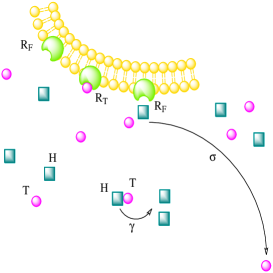
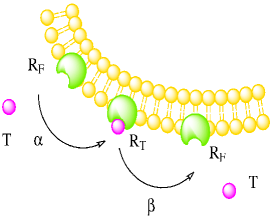
The values of $\sigma$ and $\gamma$ characterize the effectiveness of the interaction, which is in turn sensitive to the choice of the compound $T$. The idealized cartoons of figure 1 are aimed at visualizing the above reaction schemes.

$\displaystyle R_{F}+T$ $\displaystyle\stackrel{{\scriptstyle\alpha}}{{\longrightarrow}}$ $\displaystyle R_{T}+E$ $\displaystyle R_{T}+E$ $\displaystyle\stackrel{{\scriptstyle\beta}}{{\longrightarrow}}$ $\displaystyle R_{F}+T$
$\displaystyle H+T$ $\displaystyle\stackrel{{\scriptstyle\gamma}}{{\longrightarrow}}$ $\displaystyle H+H$ $\displaystyle H+T$ $\displaystyle\stackrel{{\scriptstyle\sigma}}{{\longrightarrow}}$ $\displaystyle H+E$

Figure 1: The main reaction schemes are depicted. The squares stand for the inactive species, while the circles represent the drug molecules. The model is then complemented with a set of additional reactions (see equations (2)–(5)), which accounts for the possibility that $T$ and $H$ enter (resp. leave) the region deputed for the interaction.

To complete the model we introduce an effective migration, by requiring that the $T$ and $H$ molecules can enter (resp. leave) the region deputed to the interaction. The latter assumption yields to the following set of chemical relations:

$$T \stackrel{{\scriptstyle\delta_{1}}}{{\longrightarrow}} E$$ (2)

$$E \stackrel{{\scriptstyle\eta_{1}}}{{\longrightarrow}} T$$ (3)

$$H \stackrel{{\scriptstyle\delta_{2}}}{{\longrightarrow}} E$$ (4)

$$E \stackrel{{\scriptstyle\eta_{2}}}{{\longrightarrow}} H$$ (5)

The population, namely the ensemble of elements belonging to an homologous species $X$, will be labelled in the following with the symbol $n_{X}$. Notice that the number of receptors $N_{1}=n_{R_{T}}+n_{R_{F}}$ and the total amount of molecules (including the empties) $N_{2}=n_{T}+n_{H}+n_{E}$ are conserved quantities. This observation enables us to reduce the complexity of the problem by setting:

$$n_{R_{F}}=N_{1}-n_{R_{T}}\qquad n_{E}=N_{2}-n_{T}-n_{H}$$

In the following we shall use the vectorial notation $\underline{n}=(n_{T},n_{R_{T}},n_{H})$ to help keeping the mathematical developments compact.

We are now in a position to define the transition rates $T(\underline{n}^{{}^{\prime}}|\underline{n})$ from a state $\underline{n}$ to a different one $\underline{n}^{{}^{\prime}}$. In our convention initial states are on the right and final states on the left. As an example, consider equation (1). The probability to pick up a $T$ constituents follows from simple combinatorics and reads $n_{T}/N_{2}$, while there is a probability $(N_{1}-n_{R_{T}})/N_{1}$ of $R_{F}$ being chosen. This results in $\alpha(n_{T}/N_{2})(N_{1}-n_{R_{T}})/N_{1}$ for this particular transition rate [12]. A complete listing of transition probability associated to the preceding set of chemical reactions is here enclosed:

$$T(n_{T}-1,n_{R_{T}}+1,n_{H}|\underline{n}) = \alpha\frac{n_{T}}{N_{2}}\frac{N_{1}-n_{R_{T}}}{N_{1}}$$

$$T(n_{T}+1,n_{R_{T}}-1,n_{H}|\underline{n}) = \beta\frac{N_{2}-n_{T}-n_{H}}{N_{2}}\frac{n_{R_{T}}}{N_{1}}$$

$$T(n_{T}-1,n_{R_{T}},n_{H}+1|\underline{n}) = \gamma\frac{n_{H}}{N_{2}}\frac{n_{T}}{N_{2}}$$

$$T(n_{T}-1,n_{R_{T}},n_{H}|\underline{n}) = \sigma\frac{n_{H}}{N_{2}}\frac{n_{T}}{N_{2}}+\delta_{1}\frac{n_{T}}{N_{2}}$$

$$T(n_{T}+1,n_{R_{T}},n_{H}|\underline{n}) = \eta_{1}\frac{N_{2}-n_{T}-n_{H}}{N_{2}}$$

$$T(n_{T},n_{R_{T}},n_{H}-1|\underline{n}) = \delta_{2}\frac{n_{H}}{N_{2}}$$

$$T(n_{T},n_{R_{T}},n_{H}+1|\underline{n}) = \eta_{2}\frac{N_{2}-n_{T}-n_{H}}{N_{2}}$$

Having defined the transition rates, the master equation governing the evolution of the discrete stochastic model takes the form:

$$\frac{\mathrm{d}}{\mathrm{d}t}P(\underline{n},t) = T(\underline{n}|n_{T}+1,n_{R_{T}}-1,n_{H})P(n_{T}+1,n_{R_{T}}-1,n_{H},t)$$ (6)

$$+ T(\underline{n}|n_{T}-1,n_{R_{T}}+1,n_{H})P(n_{T}-1,n_{R_{T}}+1,n_{H},t)$$

$$+ T(\underline{n}|n_{T}+1,n_{R_{T}},n_{H}-1)P(n_{T}+1,n_{R_{T}},n_{H}-1,t)$$

$$+ T(\underline{n}|n_{T}+1,n_{R_{T}},n_{H})P(n_{T}+1,n_{R_{T}},n_{H},t)$$

$$+ T(\underline{n}|n_{T}-1,n_{R_{T}},n_{H})P(n_{T}-1,n_{R_{T}},n_{H},t)$$

$$+ T(\underline{n}|n_{T},n_{R_{T}},n_{H}+1)P(n_{T},n_{R_{T}},n_{H}+1,t)$$

$$+ T(\underline{n}|n_{T},n_{R_{T}},n_{H}-1)P(n_{T},n_{R_{T}},n_{H}-1,t)$$

$$- \Big{[}T(n_{T}-1,n_{R_{T}}+1,n_{H}|\underline{n})+T(n_{T}+1,n_{R_{T}}-1,n_{H}|\underline{n})$$

$$+ T(n_{T}-1,n_{R_{T}},n_{H}+1|\underline{n})+T(n_{T}-1,n_{R_{T}},n_{H}|\underline{n})$$

$$+ T(n_{T}+1,n_{R_{T}},n_{H}|\underline{n})+T(n_{T},n_{R_{T}},n_{H}-1|\underline{n})$$

$$+ T(n_{T},n_{R_{T}},n_{H}+1|\underline{n})\Big{]}P(\underline{n},t)$$

where $P(\underline{n},t)$ is the probability to find the system in the state $\underline{n}$ at time $t$. In the next section we shall shortly report about our stochastic simulations, before turning to develop the analytical framework.

3 Numerical simulations

Based on the chemical equations introduced above, numerical simulations can be carried on, which respect the intrinsic stochastic nature of the model. To this end we employ the celebrated Gillespie algorithm [13] which exploits the information encoded in the reaction scheme to advance the system in time through a sequence of random increments. A randomly selected reaction is forced to occur during each successive step. It should be emphasized that time increments and associated reactions are chosen so to recover the exact probability distribution of the stochastic time series. For a more detail account on the philosophy of the integration recipe, the reader can consult [13].

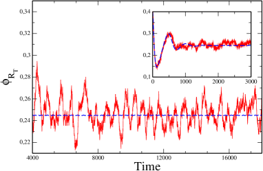
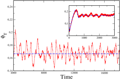
A typical result is represented in figure 2 where the normalized population of $T$-like molecules and bound receptors $R_{T}$ are reported, as function of time. Notice that large stochastic oscillations are clearly displayed, despite the relatively large number of simulated molecules. Even more interestingly, the oscillations persist when increasing the populations amount and only when a very large number of constituents is allowed, the system eventually sets down to its mean-field solution.

(a)	(b)

Figure 2: Drug molecules (panel (a)) and bound receptor (panel (b)) densities as a function of time. The solid lines refer to the time series from stochastic simulations, while the dashed lines are calculated from numerical integration of the mean field equations (4)-(9). The insets represent a zoom of the initial evolution and allow to appreciate the agreement with the mean–field solution at short times. Parameters values for both panels are $\alpha=0.008$, $\beta=0.005$, $\gamma=0.3$, $\delta_{1}=0.001$, $\delta_{2}=0.05$, $\eta_{1}=0.001$, $\sigma=0.06$, $N_{1}=5300$ and $N_{2}=20000$.

As already remarked in [12, 14, 15], this result is odds with the intuitive believe that fluctuations can be safely ignored, due to the usual statistical factor $1/\sqrt{N}$. Indeed, the observed fluctuations arise from the amplification of the intrinsic noise, associated to the discrete component of the dynamics and can potentially bear and extraordinary conceptual relevance in several applications. With reference to the case at hand, emerging, regular, oscillatory patterns in the $R_{T}$ quota, could potentially explain the modulations in the pain perception as reported in the literature, higher values of $n_{R_{T}}$ corresponding, in our interpretative scheme, to a less pronounced pain level. Alternatively, on a different time scale, the effects here discussed could provide a consistent microscopic picture to understand the presence of quasi–periodic fluctuations in the evoked electric activity of laboratory animals under anesthetic treatment.

In the forthcoming sections, we shall gain some analytical insight into the model results and characterize the specific traits of the observed oscillatory behaviors through the elegant van Kampen [7] expansion.

4 On the deterministic limit

The deterministic counterpart of the governing master equation is straightforwardly obtained as follows. Focus on $T$ and observe that, by definition:

$$\left\langle n_{T}\right\rangle=\sum_{\underline{n}}n_{T}P(\underline{n},t)$$

Multiplying equation (6) by $n_{T}$ and summing over $\underline{n}$ returns on the right–hand side $d\left\langle n_{T}\right\rangle/dt$. Simplifying the left–hand side is somehow more laborious and requires some effort. Proceeding in a completely analogous fashion for $n_{H}$ and $n_{R_{T}}$ yields to the following system of coupled differential equation for the ensemble independent variables:

$$\frac{\mathrm{d}}{\mathrm{d}t}\langle n_{T}\rangle= -\alpha\left\langle\frac{n_{T}}{N_{2}}\frac{N_{1}-n_{R_{T}}}{N_{1}}\right\rangle+\beta\left\langle\frac{N_{2}-n_{T}-n_{H}}{N_{2}}\frac{n_{R_{T}}}{N_{1}}\right\rangle-(\gamma+\sigma)\left\langle\frac{n_{H}}{N_{2}}\frac{n_{T}}{N_{2}}\right\rangle$$

$$-\delta_{1}\left\langle\frac{n_{T}}{N_{2}}\right\rangle+\eta_{1}\left\langle\frac{N_{2}-n_{T}-n_{H}}{N_{2}}\right\rangle$$

$$\frac{\mathrm{d}}{\mathrm{d}t}\langle n_{R_{T}}\rangle= \alpha\left\langle\frac{n_{T}}{N_{2}}\frac{N_{1}-n_{R_{T}}}{N_{1}}\right\rangle-\beta\left\langle\frac{N_{2}-n_{T}-n_{H}}{N_{2}}\frac{n_{R_{T}}}{N_{1}}\right\rangle$$

$$\frac{\mathrm{d}}{\mathrm{d}t}\langle n_{H}\rangle= \gamma\left\langle\frac{n_{H}}{N_{2}}\frac{n_{T}}{N_{2}}\right\rangle+\eta_{2}\left\langle\frac{N_{2}-n_{T}-n_{H}}{N_{2}}\right\rangle-\delta_{2}\left\langle\frac{n_{H}}{N_{2}}\right\rangle$$

The mean–field approximation corresponds to ignore the correlations, in the above rate equations when performing the limit for $N_{1}$ and $N_{2}$ large. Introducing $\phi_{T}=\langle n_{T}\rangle/N_{2}$, $\phi_{R_{T}}=\langle n_{R_{T}}\rangle/N_{1}$, $\phi_{H}=\langle n_{H}\rangle/N_{2}$, rescaling time as $\tau=t/N_{2}$ and formally sending $N_{1},N_{2}\rightarrow\infty$, one finally obtains:

$$\frac{\mathrm{d}}{\mathrm{d}\tau}\phi_{T}= -\alpha\phi_{T}(1-\phi_{R_{T}})+\beta\phi_{R_{T}}(1-\phi_{T}-\phi_{H})-(\gamma+\sigma)\phi_{H}\phi_{T}$$

$$-\delta_{1}\phi_{T}+\eta_{1}(1-\phi_{T}-\phi_{H})$$

$$\frac{\mathrm{d}}{\mathrm{d}\tau}\phi_{R_{T}}= c\left[\alpha\phi_{T}(1-\phi_{R_{T}})-\beta\phi_{R_{T}}(1-\phi_{T}-\phi_{H})\right]$$ (8)

$$\frac{\mathrm{d}}{\mathrm{d}\tau}\phi_{H}= \gamma\phi_{H}\phi_{T}+\eta_{2}(1-\phi_{T}-\phi_{H})-\delta_{2}\phi_{H}$$ (9)

where $c=N_{2}/N_{1}$.

We shall hereon limit our discussion to the case $\eta_{2}=0$ which will prove analytically tractable. The conclusions here demonstrated with reference to the selected case study, will obviously apply to the more general setting where fresh $H$ molecules are allowed to enter the interaction region. Investigations on the complete model ($\eta_{2}\neq 0$) will be object of a forthcoming publication.

Two fixed points, respectively labelled $\underline{\phi}_{1}^{*}$ and $\underline{\phi}_{2}^{*}$, are identified:

$$\underline{\phi}_{1}^{*}=\left(\frac{\eta_{1}}{\delta_{1}+\eta_{1}},\frac{\alpha\eta_{1}}{\beta\delta_{1}+\alpha\eta_{1}},0\right)$$

$$\underline{\phi}_{2}^{*}=\left(\frac{\delta_{2}}{\gamma},\frac{\alpha[\delta_{2}(\gamma+\sigma)+\eta_{1}\gamma]}{\alpha[\delta_{2}(\gamma+\sigma)+\eta_{1}\gamma]+\beta[(\gamma+\sigma)(\gamma-\delta_{2})+\delta_{1}\gamma]},\frac{\eta_{1}(\gamma-\delta_{2})-\delta_{1}\delta_{2}}{\delta_{2}(\gamma+\sigma)+\eta_{1}\gamma}\right)$$

In figure 2, the solid lines represent the above equilibrium solution: For such choice of the parameter, as previously mentioned, the stochastic dynamic displays macroscopic oscillation for the monitored quantities, the average reference value being correctly predicted by the mean-field theory. What is the reason for these regular fluctuation to manifest? Are they resulting from the intrinsic finite size nature of the simulated medium?

To answer these questions it is crucial to determine the stability matrix associated with the fixed points, as it will play a central role in investigating the cycling phenomenon. One can thus re–write the mean–field equations in the compact form $d\phi_{k}/d\tau=f_{k}(\underline{\phi})$, where the index $k=1,2,3$ codes the different species, namely $T$ ($k=1$), $R_{T}$ ($k=2$) and $H$ ($k=3$). The $3\times 3$ Jacobian matrix $J_{ij}=\partial f_{i}/\partial\phi_{j}|_{FP}$ (here FP means “evaluated at the fixed point”) controls the linearized dynamics about the fixed point and can be cast in the form:

$$J(\underline{\phi}^{*})=\left(\begin{array}[]{ccc}-\alpha(1-\phi_{R_{T}}^{*})-\beta\phi_{R_{T}}^{*}-(\gamma+\sigma)\phi_{H}^{*}-\delta_{1}-\eta_{1}&\alpha\phi_{T}^{*}+\beta(1-\phi_{T}^{*}-\phi_{H}^{*})&-\beta\phi_{R_{T}}^{*}-(\gamma+\sigma)\phi_{T}^{*}-\eta_{1}\\ c[\alpha(1-\phi_{R_{T}}^{*})+\beta\phi_{R_{T}}^{*}]&-c[\alpha\phi_{T}^{*}+\beta(1-\phi_{T}^{*}-\phi_{H}^{*})]&c\beta\phi_{R_{T}}^{*}\\ \gamma\phi_{H}^{*}&0&\gamma\phi_{T}^{*}-\delta_{2}\end{array}\right)$$ (10)

One can easily show that $J(\phi^{*}_{1})$ admits two real negative eigenvalues and a third one, also real, whose sign depends on the choice of the parameters. A stability analysis for the second equilibrium point proves technically difficult. However, via numerical inspections, a large region in the parameters’ space is identified, which yields to complex solutions. In particular, complex eigenvalues of the $J(\phi^{*}_{2})$ are found having negative real part. This condition ensures an oscillatory approach to equilibrium, a fundamental ingredient which is eventually responsible for the large scale modulations observed in the finite size regime. Tracing the region in space deputed to the aforementioned behavior falls out of the scope of the present paper and shall be postponed to a forthcoming contribution together with a detailed characterization of the general case with $\eta_{2}\neq 0$.

Following the above, from now on, we shall denote with $\underline{\phi}^{*}$ a particular value of $\underline{\phi}^{*}_{2}$ for which damped oscillations do occur in the mean–field scenario.

5 Characterizing the fluctuations: The van Kampen expansion

As clearly depicted in figure 2 the innate discreteness of the stochastic medium drives into the system important effects which cannot be captured within the continuous mean–field scenario. To shed light into the observed phenomena we can bring into the game the fluctuations by performing the following explicit replacement:

$$n_{T}=N_{2}\phi_{T}(t)+\sqrt{N_{2}}\xi_{T}\quad n_{R_{T}}=N_{1}\phi_{R_{T}}(t)+\sqrt{N_{1}}\xi_{R_{T}}\quad n_{H}=N_{2}\phi_{H}(t)+\sqrt{N_{2}}\xi_{H}$$ (11)

where the new continuous variable $\underline{\xi}=(\xi_{T},\xi_{R_{T}}\xi_{R_{H}})$ replace the discrete quantity $\underline{n}=(n_{T},n_{R_{T}},n_{H})$ in the definition the probability distribution, namely $P(\underline{n},t)=\Pi(\underline{\xi},\tau)$.

Before proceeding, it is worth emphasizing that the $1/\sqrt{N_{1}}$ (resp. $1/\sqrt{N_{2}}$) term holds because of the central-limit theorem: The fluctuations are in fact expected to decay in a similar fashion and, in the continuous limit, $N_{1},N_{2}\rightarrow\infty$ the system is entirely characterized in term of its continuous variables $\underline{\phi}=(\phi_{T},\phi_{R_{T}},\phi_{H})$ as prescribed by equations (11).

The master equation can be re-written as function of the new variables. The left-hand side reads:

$$\frac{\mathrm{d}}{\mathrm{d}t}P(\underline{n},t)=\frac{1}{N_{2}}\frac{\partial\Pi}{\partial\tau}-\frac{1}{\sqrt{N_{2}}}\frac{\mathrm{d}}{\mathrm{d}\tau}\phi_{T}\frac{\partial\Pi}{\partial\xi_{T}}-\frac{c^{-1}}{\sqrt{N_{1}}}\frac{\mathrm{d}}{\mathrm{d}\tau}\phi_{R_{T}}\frac{\partial\Pi}{\partial\xi_{R_{T}}}-\frac{1}{\sqrt{N_{2}}}\frac{\mathrm{d}}{\mathrm{d}\tau}\phi_{H}\frac{\partial\Pi}{\partial\xi_{H}}$$

where use has been made of the fact that the time derivative is taken at constant $\underline{n}$. The right-hand side follows from a straightforward, though lengthy, application of the large-$N$ van Kampen expansion. The main step of the derivation are reviewed in the appendix. The interested reader can refer to [7, 16] for a detailed account on the whole procedure.

At leading order of the expansion we recover the deterministic mean–field equations (4)–(9), while at next–to–leading order we obtain the linear multivariate Fokker Planck equation (19) that governs the evolution of the fluctuations. The coefficients of this equation are completely specified as function of the model’s parameters (see the appendix): In principle, by solving equation (19) we are in a position to quantify the deviation from the ideal mean–field dynamics, via the probability distribution $\Pi$. At present, we aim at understanding the oscillation and, to this end, we invoke a completely equivalent formulation of the Fokker Planck equation. The problem can be in fact cast as a set of stochastic differential equations of Langevin type, which take the explicit form:

$$\frac{d\xi_{i}}{d\tau}=A_{i}(\underline{\xi})+\eta_{i}(\tau)\qquad i=1,..,3$$ (12)

where for convenience, as a natural extension of the notation introduce above, we have now set $\xi_{1}=\xi_{T}$, $\xi_{2}=\xi_{R_{T}}$, $\xi_{3}=\xi_{H}$ and $A_{i}$ is specified in the appendix. The term $\eta_{i}$ is a Gaussian noise with zero mean and with correlation given by

$$\langle\eta_{i}(\tau)\eta_{j}(\tau^{{}^{\prime}})\rangle=B_{ij}\delta(\tau-\tau^{{}^{\prime}})$$

To highlight the existence of a possible oscillatory behavior we perform a Fourier analysis of equations (12), and obtain:

$$-i\omega\tilde{\xi}_{i}(\omega)=\sum_{j}M_{ij}\tilde{\xi}_{j}(\omega)+\tilde{\eta}_{i}(\omega)$$

where the tilde stands for the Fourier transform. Following [15] we can re-write this as:

$$\sum_{j}\Phi_{ij}(\omega)\tilde{\xi}_{j}(\omega)=\tilde{\eta}_{i}(\omega)$$ (13)

with $\Phi_{ij}(\omega)=-i\omega\delta_{ij}-M_{ij}$. In addition one gets:

$$\langle\tilde{\eta}_{i}(\omega)\tilde{\eta}_{j}(\omega^{{}^{\prime}})\rangle=B_{ij}(2\pi)\delta(\omega+\omega^{{}^{\prime}})$$

Solving equation (13) for $\tilde{\xi}_{i}$ and computing the power spectrum results in:

$$P_{i}(\omega)=\langle|\tilde{\xi}_{i}(\omega)|^{2}\rangle=\sum_{j}\sum_{k}\Phi_{ij}^{-1}(\omega)B_{jk}(\Phi_{ij}^{\dagger})^{-1}(\omega)$$ (14)

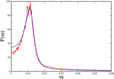
where we have used $\Phi_{ij}^{\dagger}(\omega)=\Phi_{ji}(-\omega)$. The power spectrum predicted by equation (14) is plotted in figure 3, for the same set of parameters as employed in the simulations of figure 2. A clear peak is detected. Moreover, the theoretical curve interpolates correctly the numerical profile. These results confirm that the macroscopic oscillations which manifest in the acquired time-series stem from the noise intrinsic to the system under investigation. It is our believe that mechanisms similar to the ones here hypothesized, are potentially in place in the complex human (animal) body environment and could in principle form the basis of a consistent molecular interpretation for the large collection of experimental, biomedical observations to which we made reference in the introductory section.

Figure 3: A plot of the power spectrum $P(\omega)$ for the $R_{T}$ time series as a function of the frequency $\omega$. The noisy line corresponds to the spectrum calculated from 500 runs of the stochastic simulation of the model. The smooth line shows the analytic prediction from equation (14). For the parameters’ setting refer to the caption of figure 2.

6 Conclusions

In this paper we propose a discrete dynamical framework which is aimed at shedding new light onto the complex molecular processes intervening in response to an external harming stimulus so to trigger the pain sensation. We are in particular interested in elucidating the crucial interplay between the administered drug molecules, which express their analgesic function chasing the target receptors, and other chemical elements freely diffusing in the stream. The latter can substantially reduce the anaesthetic effect, by hindering the available binding sites. Similarly, drug molecules can be turned into inactive species following binary encounters. The mechanisms here postulated are formally coded via chemical reactions and define a consistent stochastic scheme. Numerical simulations display macroscopic oscillations in the concentration amount: the number of bound receptors change cyclically in time, a trend which we assume to induce an analogous modulation for the experienced perception of pain. These findings are analytically illustrated by developing a large-size expansion which enables us to predict the existence of a peaked power spectrum. It is important to remark that the amplification process here discussed stems from the underlying stochasticity, which excites the resonant frequencies of the system. Oscillations arise hence naturally, driven by the noise which is intrinsic to the system and without invoking any ad hoc couplings among the molecular agents participating to the dynamics. Our findings could suggest the existence of a simple, though general, molecular mechanism responsible for the emergence of cyclic behaviors in response to analgesic treatments [5]. We shall here stress that our main conclusions apply also for the more general setting where $\eta_{2}\neq 0$. In particular the peaked power spectrum is also found in this latter case and the region in the parameters’ space which corresponds to the emergence of the cycles can be partially identified on the basis of explicit analytic formulae. These findings will be reported in a forthcoming publication [17].

Appendix

The first technical point of the van Kampen expansion concerns the introduction of the so–called shift operators, $\mathbb{E}^{\pm 1}_{T},\mathbb{E}^{\pm 1}_{R_{T}},\mathbb{E}^{\pm 1}_{H}$ which obey:

$$\mathbb{E}^{\pm 1}_{T}f(\underline{n},t)=f(n_{T}\pm 1,n_{RT},n_{H})$$

$$\mathbb{E}^{\pm 1}_{R_{T}}f(\underline{n},t)=f(n_{T},n_{RT}\pm 1,n_{H})$$

$$\mathbb{E}^{\pm 1}_{H}f(\underline{n},t)=f(n_{T},n_{RT},n_{H}\pm 1)\>.$$

The master equation (6) is hence cast in the form:

$$\frac{1}{N_{2}}\frac{\partial\Pi}{\partial\tau} - \frac{1}{\sqrt{N_{2}}}\frac{\mathrm{d}}{\mathrm{d}\tau}\phi_{T}\frac{\partial\Pi}{\partial\xi_{T}}-\frac{c^{-1}}{\sqrt{N_{1}}}\frac{\mathrm{d}}{\mathrm{d}\tau}\phi_{R_{T}}\frac{\partial\Pi}{\partial\xi_{R_{T}}}-\frac{1}{\sqrt{N_{2}}}\frac{\mathrm{d}}{\mathrm{d}\tau}\phi_{H}\frac{\partial\Pi}{\partial\xi_{H}}=$$ (15)

$$+ (\mathbb{E}^{+1}_{T}\mathbb{E}^{-1}_{R_{T}}-1)\left[\alpha\left(1-\phi_{R_{T}}-\frac{1}{\sqrt{N_{1}}}\xi_{R_{T}}\right)\left(\phi_{T}+\frac{1}{\sqrt{N_{2}}}\xi_{T}\right)\Pi\right]$$

$$+ (\mathbb{E}^{-1}_{T}\mathbb{E}^{+1}_{R_{T}}-1)\left[\beta\left(\phi_{R_{T}}+\frac{1}{\sqrt{N_{1}}}\xi_{R_{T}}\right)\left(1-\phi_{T}-\frac{1}{\sqrt{N_{2}}}\xi_{T}-\phi_{H}-\frac{1}{\sqrt{N_{2}}}\xi_{H}\right)\Pi\right]$$

$$+ (\mathbb{E}^{+1}_{T}\mathbb{E}^{-1}_{H}-1)\left[\gamma\left(\phi_{T}+\frac{1}{\sqrt{N_{2}}}\xi_{T}\right)\left(\phi_{H}+\frac{1}{\sqrt{N_{2}}}\xi_{H}\right)\Pi\right]$$

$$+ (\mathbb{E}^{+1}_{T}-1)\left[\sigma\left(\phi_{T}+\frac{1}{\sqrt{N_{2}}}\xi_{T}\right)\left(\phi_{H}+\frac{1}{\sqrt{N_{2}}}\xi_{H}\right)\Pi+\delta_{1}\left(\phi_{T}+\frac{1}{\sqrt{N_{2}}}\xi_{T}\right)\Pi\right]$$

$$+ (\mathbb{E}^{-1}_{T}-1)\left[\eta_{1}\left(1-\phi_{T}-\frac{1}{\sqrt{N_{2}}}\xi_{T}-\phi_{H}-\frac{1}{\sqrt{N_{2}}}\xi_{H}\right)\Pi\right]$$

$$+ (\mathbb{E}^{+1}_{H}-1)\left[\delta_{2}\left(\phi_{H}+\frac{1}{\sqrt{N_{2}}}\xi_{H}\right)\Pi\right]$$

The advantage of using the shift operators relies in that they admit a simple expansion in the limit for $N_{1}$ (resp. $N_{2}$) large:

$$\mathbb{E}^{\pm 1}_{T}=1\pm N_{2}^{-1/2}\frac{\partial}{\partial\xi_{T}}+\frac{1}{2}N_{2}^{-1}\frac{\partial^{2}}{\partial\xi_{T}^{2}}\pm\cdots$$ (16)

$$\mathbb{E}^{\pm 1}_{R_{T}}=1\pm N_{1}^{-1/2}\frac{\partial}{\partial\xi_{R_{T}}}+\frac{1}{2}N_{1}^{-1}\frac{\partial^{2}}{\partial\xi_{R_{T}}^{2}}\pm\cdots$$ (17)

$$\mathbb{E}^{\pm 1}_{H}=1\pm N_{2}^{-1/2}\frac{\partial}{\partial\xi_{H}}+\frac{1}{2}N_{2}^{-1}\frac{\partial^{2}}{\partial\xi_{H}^{2}}\pm\cdots$$ (18)

Plugging (16)-(18) into (15), after some algebraic manipulation, one recovers at the leading order the mean–field equations, formally identical to the ones reported above, see equations (4)-(9). The next–to–leading order result in a Fokker Planck equation for the probability distribution $\Pi(\underline{\xi},t)$:

$$\frac{\partial\Pi}{\partial\tau}=-\sum_{i}\frac{\partial}{\partial\xi_{i}}\left(A(\underline{\xi})\Pi\right)+\frac{1}{2}\sum_{ij}B_{ij}\frac{\partial^{2}\Pi}{\partial\xi_{i}\partial\xi_{j}}$$ (19)

where:

$$A(\underline{\xi})=\sum_{j}M_{ij}\xi_{j}$$

with

$$M=\left(\begin{array}[]{ccc}-\alpha(1-\phi_{R_{T}}^{*})-\beta\phi_{R_{T}}^{*}-(\gamma+\sigma)\phi_{H}^{*}-\delta_{1}-\eta_{1}&c^{1/2}[\alpha\phi_{T}^{*}+\beta(1-\phi_{T}^{*}-\phi_{H}^{*})]&-\beta\phi_{R_{T}}^{*}-(\gamma+\sigma)\phi_{T}^{*}-\eta_{1}\\ c^{1/2}[\alpha(1-\phi_{R_{T}}^{*})+\beta\phi_{R_{T}}^{*}]&-c[\alpha\phi_{T}^{*}+\beta(1-\phi_{T}^{*}-\phi_{H}^{*})]&c^{1/2}\beta\phi_{R_{T}}^{*}\\ \gamma\phi_{H}^{*}&0&\gamma\phi_{T}^{*}-\delta_{2}\end{array}\right)$$

Notice that for $c=1$ (see [14]), $M$ reduces to the Jacobian matrix (10) which can be directly calculated from the mean–field system. $B$ is instead a symmetric matrix whose elements reads:

$$B_{11} =\alpha\phi_{T}^{*}(1-\phi_{R_{T}}^{*})+\beta\phi_{R_{T}}^{*}(1-\phi_{T}^{*}-\phi_{H}^{*})+(\gamma+\sigma)\phi_{T}^{*}\phi_{H}^{*}+\delta_{1}\phi_{T}^{*}+\eta_{1}(1-\phi_{T}^{*}-\phi_{H}^{*})$$

$$B_{12} =-c^{1/2}[\alpha\phi_{T}^{*}(1-\phi_{R_{T}}^{*})+\beta\phi_{R_{T}}^{*}(1-\phi_{T}^{*}-\phi_{H}^{*})]$$

$$B_{13} =-\gamma\phi_{T}^{*}\phi_{H}^{*}$$

$$B_{22} =c[\alpha\phi_{T}^{*}(1-\phi_{R_{T}}^{*})+\beta\phi_{R_{T}}^{*}(1-\phi_{T}^{*}-\phi_{H}^{*})]$$

$$B_{23} =0$$

$$B_{33} =\gamma\phi_{T}^{*}\phi_{H}^{*}+\delta_{2}\phi_{H}^{*}$$

References

• [1] Victor M and Ropper A H. Principles Of Neurology. McGraw–Hill, 2001.
• [2] Misulis K E and Fakhoury T. Spehlmann’s Evoked Potential Primer. Butterworth–Heinemann, 3rd edition, 2001.
• [3] De Pascalis V and Cacace I. Pain perception, obstructive imagery and phase–ordered gamma oscillations. Int. J. Psychophysiol., 56:157–169, 2005.
• [4] Gross J, Schnitzler A, Timmermann L, and Ploner M. Gamma oscillations in human primary somatosensory cortex reflect pain perception. PLoS Biol., 5:1168–1173, 2007.
• [5] Rojas M J, Navas J A, and Rector D M. Evoked response potential markers for anesthetic and behavioral states. Am. J. Physiol. Regul. Integr. Comp. Physiol., 291:R189–R196, 2006.
• [6] Danhof M, de Jongh J, De Lange E C M, Della Pasqua O, Ploeger B A, and Voskuyl R A. Mechanism–based pharmacokinetic–pharmacodynamic modeling: Biophase distribution, receptor theory, and dynamical systems analysis. Annu. Rev. Pharmacol. Toxicol., 47:357–400, 2007.
• [7] van Kampen N G. Stochastic preocesses in Physics and Chemistry. North Holland, Amsterdam, 1992.
• [8] Grond S and Sablotzki A. Clinical pharmacology of tramadol. Clin. Pharmacokinet., 43:879–923, 2004.
• [9] Gillen C, Haurand M, Kobelt D J, and Wnendt S. Affinity, potency and efficacy of tramadol and its metabolites at the cloned human μ𝜇\mu–opiod receptor. Naunyn–Schmiedeberg’s Arch. Pharmacol., 362:116–121, 2000.
• [10] Katzung B G. Basic & Clinical Pharmacology. McGraw-Hill, 9th edition, 2004.
• [11] Lintz W, Barth H, Osterloh G, and Schmidt-Bothelt E. Bioavailability of enteral tramadol formulations. 1st communication: capsules. Arzneimittelforschung, 36:1278–1283, 1986.
• [12] McKane A J and Newman T J. Stochastic models in population biology and their deterministic analogs. Phys. Rev. E, 70:041902, 2004.
• [13] Gillespie D T. A general method for numerically simulating the stochastic time evolution of coupled chemical reactions. J. Comp. Phys., 22:403–434, 1976.
• [14] McKane A J and Newman T J. Predator-prey cycles from resonant amplification of demographic stochasticity. Phys. Rev. Lett., 94:218102, 2005.
• [15] McKane A J, Nagy J D, Newman T J, and Stefanini M O. Amplified biochemical oscillations in cellular systems. J. Stat. Phys., 128:165–191, 2007.
• [16] Gardiner C W. Handbook of Stochastic Methods. Springer, second edition, 1985.
• [17] Di Patti F and Fanelli D. In preparation.