Photometric constraints on white dwarfs and the identification of extreme objects

Abstract

It is possible to reliably identify white dwarfs (WDs) without recourse to spectra, instead using photometric and astrometric measurements to distinguish them from Main Sequence stars and quasars. WDs’ colours can also be used to infer their intrinsic properties (effective temperature, surface gravity, etc.), but the results obtained must be interpreted with care. The difficulties stem from the existence of a solid angle degeneracy, as revealed by a full exploration of the likelihood, although this can be masked if a simple best-fit approach is used. Conversely, this degeneracy can be broken if a Bayesian approach is adopted, as it is then possible to utilise the prior information on the surface gravities of WDs implied by spectroscopic fitting. The benefits of such an approach are particularly strong when applied to outliers, such as the candidate halo and ultra-cool WDs identified by Vidrih et al. (2007). A reanalysis of these samples confirms their results for the latter sample but suggests that that most of the halo candidates are thick disk WDs in the tails of the photometric noise distribution.

1 Introduction

White dwarfs (WDs) are sufficiently long-lived that they can be used to measure the Galaxy’s age (e.g., Fontaine et al. 2001, 2005 and references therein) and star-formation history (e.g., Wood 1992), and can even be used as cosmological probes (e.g., Bergeron et al. 1997; Leggett et al. 1998; Harris et al. 1999; Hodgkin et al. 2000; Gates et al. 2004; Harris et al. 2008). WDs in the Galaxy’s halo have also been invoked as potential dark matter candidates (e.g., Oppenheimer et al. 2001a; Oppenheimer et al. 2001b), although these claims are the subject of considerable debate (e.g., Reid 2005 and references therein).

All such investigations rely on being able to constrain a WD’s properties: its distance, $D$, and its intrinsic parameters (effective temperature, $T_{\mathrm{eff}}$; surface gravity, $g$; absolute magnitude, $M_{\mathrm{bol}}$; radius, $R$; atmospheric composition; etc.). The distances to a number of the closest WDs (with $D\la 100{\mbox{\rm\,\,pc}}$) have been determined unambiguously by parallax measurements (e.g., Bergeron et al. 2001), and the Gaia satellite (Perryman et al., 2001) will eventually measure parallaxes for all Galactic sources brighter than $r\simeq 20$ (e.g., Torres et al. 2005; Jordan 2007). In most cases, however, the characterisation of WDs is necessarily more model-dependent, with spectroscopic or photometric data used to infer the physical properties of WDs. WD spectra encode sufficient information to infer $T_{\mathrm{eff}}$ and $\log{\mbox{\em{g}}}$ to a relative accuracy of $\la 10$ per cent (e.g., Bergeron et al. 1992; McCook & Sion 1999; Harris et al. 2003; Kleinman et al. 2004; Eisenstein et al. 2006), and the agreement between the various semi-independent models (e.g., Bergeron et al. 1995; Finley et al. 1997; Fontaine et al. 2001; Bergeron et al. 2001; Bergeron & Leggett 2002; Holberg & Bergeron 2006) gives grounds for confidence in the resultant parameter estimates. Perhaps the most impressive demonstration of spectroscopic fitting has been the largely automated analysis of $\sim 10^{4}$ Sloan Digital Sky Survey (SDSS; York et al. 2000) WDs by Eisenstein et al. (2006). This confirmed that most WDs have $\log{\mbox{\em{g}}}\simeq 8$ (cf. Bergeron et al. 1992; Liebert et al. 2005), but also that the inferred surface gravities and masses of cool ($T_{\mathrm{eff}}\la 10^{4}{\mbox{\rm\,\,K}}$) WDs can be biased high (cf. Bergeron et al. 1990; Kleinman et al. 2004; Eisenstein et al. 2006). Interestingly, such a bias is not seen in purely photometric fits (Engelbrecht & Koester, 2007). Combined with the fact that it is possible to reliably identify WDs using only photometric and astrometric data (e.g., Harris et al. 2006; Kilic et al. 2006), it is of great importance to understand what constraints can be placed on a WD’s properties from photometric data alone.

Figure 1: Two colour diagrams for a sample of non-variable point–sources in SDSS Stripe 82 from Ivezić et al. (2007). In (a) and (c) the sources have relative photometric errors of $\sim 0.01$ in all bands; in (b) the errors have been inflated to be $\sim 0.05$. The Fontaine–Bergeron model grids for H (red) and He (blue) WDs are also shown, the temperature going from $T_{\mathrm{eff}}=110000{\mbox{\rm\,\,K}}$ at the bottom-left down to $T_{\mathrm{eff}}\simeq 6000{\mbox{\rm\,\,K}}$ at the top-right, with the exception of the coolest H models in (c).

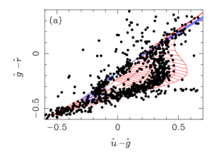
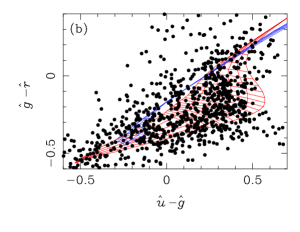
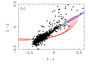
The most optimistic case is illustrated in Fig. 1 (a), in which colour measurements of non-variable point–sources generated from multi-epoch SDSS Stripe 82 data by Ivezić et al. (2007) are compared to predicted photometry generated by G. Fontaine and P. Bergeron. The sources shown have relative photometric errors of $\sim 0.01$ in all bands, and are mainly WDs, although there is some contamination at high $g$$-$$r$ from quiescent quasars (Sesar et al., 2007) and unresolved pairs of white and red dwarfs (Smolčić et al., 2004). Comparison of the observed WD loci with the models in Fig. 1 (a) reveals not only an obvious separation between the H and He WDs, but also clear differentiation in $T_{\mathrm{eff}}$. The surface gravity is well constrained for H atmosphere WDs with $10^{4}{\mbox{\rm\,\,K}}\la T_{\mathrm{eff}}\la 2\times 10^{4}{\mbox{\rm\,\,K}}$ (i.e., $\mbox{\mbox{$u$}$-$$\mbox{$g$}$}\simeq 0.3$ and $\mbox{\mbox{$g$}$-$$\mbox{$r$}$}\simeq-0.2$). Unfortunately, this level of characterisation, particularly in $\log{\mbox{\em{g}}}$, relies on Stripe 82’s near-ideal combination of photometric precision and wavelength coverage. Fig. 1 (b) shows the results of increasing the relative photometric errors of the Stripe 82 data to $\sim 0.05$: the H and He loci are no longer discernable and only the broadest constraints could be placed on $\log{\mbox{\em{g}}}$ from these data. Even more critical than high photometric precision is access to near-ultraviolet (NUV) data, as can be seen from Fig. 1 (c). In the longer wavelength optical bands WDs’ colours depend primarily on $T_{\mathrm{eff}}$, with minimal separation in $\log{\mbox{\em{g}}}$, or between H and He models.

However even non-ideal observations of the sort shown in Fig. 1 (b) or (c) would allow $T_{\mathrm{eff}}$ to be constrained, provided only that the WD is uambiguously detected (i.e., with relative photometric errors of $\la 0.1$) in at least two passbands that are blueward of its Rayleigh–Jeans tail. In this situation the only other available information comes from the flux measurements, which then fix the solid angle, $\Omega$, subtended by the source. As

$$\Omega\propto\frac{R^{2}}{D^{2}}\propto\frac{M}{gD^{2}}\propto\frac{M}{10^{\log{\mbox{\em{g}}}}D^{2}},$$ (1)

this leads to a well-known degeneracy between distance and radius, and hence surface gravity, that is difficult to break with photometric data alone (e.g., Bergeron et al. 1997, 2001). It is, however, possible to use prior knowledge of the Galactic WD population – specifically, that most WDs have $\log{\mbox{\em{g}}}\simeq 8$ – to break this degeneracy. Harris et al. (2006) adopted this approach in their analysis of a large sample of photometric SDSS WDs by assuming $\log{\mbox{\em{g}}}=8$, although it is undoubtedly overly-prescriptive to deny any possibility that a WD’s surface gravity deviates from this fiducial value. Nonetheless, this is more realistic than the alternative of treating all $\log{\mbox{\em{g}}}$ values as equally likely a priori; this assumption was made by Vidrih et al. (2007), hereafter V07, in their analysis of a (different) photometric SDSS WD sample. Both Harris et al. (2006) and V07 identified possible halo WDs, although the existence of a strong parameter degeneracy means that the identification of outliers on the basis of best-fit parameter estimates is likely to yield large numbers of spurious candidates.

The overall implication is that any non-spectroscopic WD parameter estimates will depend in part on the fitting procedure used, and that prior information about the Galactic WD population could be as important as the data that are specific to the source in question. At least some of these issues can be resolved by adopting a more rigorous statistical approach to estimating WD parameters from photometric and astrometric data. This rather broad topic will be addressed in a series of papers, of which this is the first. It deals with the more focussed question: How much can be inferred about a WD from photometric data alone? After describing the Bayesian formalisms for parameter estimation (Section 2) and model selection (Section 3), the WD population model used as a prior distribution is developed in Section 4. After analysing simulated WD observations (Section 5), these methods are applied to the small samples of candidate halo and ultra-cool WDs identified by V07 in Section 6. The conclusions and future directions of this research are summarised in Section 7.

2 Parameter estimation

Given photometry of a WD [i.e., measured apparent magnitudes, $\mbox{\boldmath${\mbox{\boldmath${d}$}}$}=(\hat{m}_{1},\hat{m}_{2},\ldots,\hat{m}_{N_{b}})$, in each of $N_{\mathrm{b}}$ bands], what constraints can be placed on its properties [i.e., the model parameters $\mbox{\boldmath${\theta}$}=(g,T_{\mathrm{eff}},D)$], assuming its dominant atmospheric element (H or He) is known? This is a classic parameter estimation problem for which several approaches exist; central to all of them is the sampling distribution, or likelihood, which gives the probability of observing the data ${d}$ given a model ${\theta}$. For the high signal–to–noise ratio measurements considered here, the likelihood has the form

$$L(\mbox{\boldmath${d}$}|\mbox{\boldmath${\theta}$}) = L\left(\hat{m}_{1},\hat{m}_{2},\ldots,\hat{m}_{N_{b}}|g,T_{\mathrm{eff}},D\right)$$ (2)

$$= \prod_{b=1}^{N_{b}}\frac{1}{(2\pi)^{1/2}\Delta\hat{m}_{b}}\exp\left(-\chi^{2}_{b}/2\right),$$

where

$$\chi^{2}_{b}=\left\{\frac{\hat{m}_{b}-\left[M_{b}(g,T_{\mathrm{eff}})+5\log(D/10{{\mbox{\rm\,\,pc}}})\right]}{\Delta\hat{m}_{b}}\right\}^{2},$$ (3)

$\Delta\hat{m}_{b}$ is the estimated noise in the $b$th band and $M_{b}(g,T_{\mathrm{eff}})$ is given by interpolating between a grid of WD models. The effects of the interstellar medium (ISM) are ignored here, but could be incorporated into Eq. (3) by adding a band-dependent extinction term inside the square brackets to account for the extra dimming.

It is at this point that the various methods of parameter estimation diverge. Historically, the most common approach has been to use one of several best-fit estimators (Section 2.1), although it is possible to obtain more reliable parameter values and uncertainties using Bayesian inference (Section 2.2).

2.1 Best-fit parameter estimation

An intuitively appealing and commonly used method of parameter estimation is to find the model, $\hat{\mbox{\boldmath${\theta}$}}$, that is the best fit to the data. This can be found in several different ways, including maximizing the likelihood, minimizing $\chi^{2}$, or by a least squares approach, all of which are equivalent for the simple sampling distribution given in Eq. (2). The large WD samples identified by Kilic et al. (2006), Harris et al. (2006) and V07 were analysed using variants of this approach, although Harris et al. (2006) restricted their investigation to models with $\log{\mbox{\em{g}}}=8$ and V07 examined only models on Bergeron’s grid of pre-computed values. Harris et al. (2006) do not quote uncertainties, and a heuristic procedure to obtain uncertainties is used in V07, whereby the best and second-best fitting grid points are compared. Given the fundamental reduction in precision attainable when using only photometric data to constrain the properties of WDs, it is clearly important to investigate this issue more thoroughly.

2.2 Inferential parameter estimation

In order to obtain the tightest possible constraints on model parameters all the available information must be utilised, which implies that any prior knowledge of the model parameters must be included (which is also necessary for self-consistency; e.g., Jaynes 2003). Applying Bayes’s theorem to the data, ${d}$, yields the posterior probability distribution

$$P(\mbox{\boldmath${\theta}$}|\mbox{\boldmath${d}$})=\frac{\pi(\mbox{\boldmath${\theta}$})L(\mbox{\boldmath${d}$}|\mbox{\boldmath${\theta}$})}{E(\mbox{\boldmath${d}$})},$$ (4)

where $\pi(\mbox{\boldmath${\theta}$})$ is the prior probability distribution of the parameters, $L(\mbox{\boldmath${d}$}|\mbox{\boldmath${\theta}$})$ is the likelihood, given in Eq. (2), and the evidence is the integral over the $N_{\mathrm{p}}$ model parameters,

$$E(\mbox{\boldmath${d}$})=\int\pi(\mbox{\boldmath${\theta}$})L(\mbox{\boldmath${d}$}|\mbox{\boldmath${\theta}$})\,{\mathrm{d}}\theta_{1}\,{\mathrm{d}}\theta_{2}\,\ldots\,{\mathrm{d}}\theta_{N_{\mathrm{p}}}.$$ (5)

The evidence plays an important role in model selection (Section 3), but in parameter estimation serves only to normalise the posterior, and so it is often more convenient to work with the unnormalised posterior, defined most simply as

$$P^{\prime}(\mbox{\boldmath${\theta}$}|\mbox{\boldmath${d}$})=\pi(\mbox{\boldmath${\theta}$})L(\mbox{\boldmath${d}$}|\mbox{\boldmath${\theta}$}).$$ (6)

Formally, the entire posterior distribution is the Bayesian answer to any parameter estimation problem, but even though it can be written down directly it is not always useful in practice. Even with just three model parameters, a numerical algorithm is required to determine the location and extent of the posterior peak – and the peak is not necessarily well-defined in the presence of degeneracies. Instead, it is far more efficient to explore the parameter space using Markov chain Monte Carlo (MCMC, e.g., Neal 1993; Gilks et al. 1999) techniques. Many different MCMC algorithms exist, although all have the same aim: to generate a sample of model parameter values, $\{\mbox{\boldmath${\theta}$}_{1},\mbox{\boldmath${\theta}$}_{2},\mbox{\boldmath${\theta}$}_{3},\ldots\}$, drawn from the posterior distribution. For the problem at hand, a fairly simple implementation of the Metropolis–Hastings algorithm (Metropolis et al. 1953; Hastings 1970) is sufficient, in which the posterior is sampled by a guided random walk that tends to explore the high posterior regions whilst occasionally exploring the low probability tails of the distribution. The samples generated from the first stage of this process (burn in) must be discarded, as they are determined partly by the starting value, but eventually the statistical properties of the chain will depend on $P^{\prime}(\mbox{\boldmath${\theta}$}|\mbox{\boldmath${d}$})$ alone. Whilst there are only heuristic tests to identify these two phases of the MCMC process (e.g., Gelman, A. and Rubin, D. B. 1992) a brute force approach can be used to ensure that the final chain is well-mixed.

A Markov chain of samples from the posterior has a number of desirable properties, one of the most fundamental being that it already samples all of the possible sub-sets of model parameters, a task that otherwise would require a multi-dimensional marginalisation integral over the other parameters. Another advantage of the Monte Carlo approach is that the distribution of not only the independent model parameters (i.e., $g$, $T_{\mathrm{eff}}$ and $D$ here) but of any derived parameters (e.g., mass, $M$, or radius, $R$) can be obtained simply by calculating the value of interest for each sample drawn from the posterior.

In many situations – in particular that considered here, in which chains are generated for each WD in a large sample – it is impractical to store the full chains. If the posterior is sufficiently localised then it is generally more useful to obtain a fiducial parameter estimate, $\hat{\mbox{\boldmath${\theta}$}}$, and uncertainty, $\Delta\hat{\mbox{\boldmath${\theta}$}}$, from the chain. As the full Bayesian answer to any parameter estimation problem is the entire posterior distribution, there can be no single correct approach; but several algorithms give reasonable approximations to single-peaked posteriors. The simplest is to take moments of the distribution, thus identifying the mean of the distribution as the fiducial estimate $\hat{\mbox{\boldmath${\theta}$}}$ and using the variance to obtain $\Delta\hat{\mbox{\boldmath${\theta}$}}$. Whilst this approach is appealingly straightforward, it has the disadvantage of being sensitive to outliers (which can occasionally be extreme, due to the stochastic nature of the MCMC algorithm). A more robust method of generating parameter estimates and uncertainties is to use the median value in each model parameter to construct $\hat{\mbox{\boldmath${\theta}$}}$ and then integrate the marginalised probability outwards in each direction to enclose the desired fraction of the posterior. This approach is adopted here, with the quoted uncertainties enclosing the central 68 per cent of the marginalised probability in the parameter of interest.

3 Model selection

Section 2 addressed the question of how to estimate the parameters of a WD given its dominant atmospheric element, but the same data can also be used to determine the likely atmospheric composition (or even whether the object is a WD at all, although this possibility is not explored here). The conventional method of model comparison (Section 3.1) uses only the quality of the best fit under the different hypotheses, whereas the Bayesian approach marginalises over the model parameters and also includes a prior on each model (Section 3.2).

3.1 Best-fit model selection

The most common approach to model comparison is to use the best-fit statistics described in Section 2.1 to characterise how well the models fit the data. In the simple case under consideration here (i.e., in which the two models have the same parameters) the resultant model comparison statistic typically reduces to the likelihood ratio,

$$\frac{L_{\mathrm{max,{\mathrm{H}}}}}{L_{\mathrm{max,{\mathrm{He}}}}}=\exp\left[-\frac{1}{2}(\chi^{2}_{\mathrm{min,{\mathrm{H}}}}-\chi^{2}_{\mathrm{min,{\mathrm{He}}}})\right],$$ (7)

where the right hand expression assumes the likelihood has the form of Eq. (2). In some simple situations this is a sufficient statistic for model comparison, but the fact that it only encodes information about a single point in parameter space means that it is of limited utility in general.

3.2 Inferential model selection

The central relationship in Bayesian model selection (e.g., Jaynes 2003) is, as in Section 2.2, Bayes’s theorem, this time applied to the discrete hypotheses that the WD atmosphere is predominantly H or He. Given data ${d}$ and the model parameters ${\theta}$ (which, in this case, are the same for both hypotheses), the probability that the WD atmosphere is H is

$$P_{\mathrm{H}}(\mbox{\boldmath${d}$})=\frac{\pi_{\mathrm{H}}E_{\mathrm{H}}(\mbox{\boldmath${d}$})}{\pi_{\mathrm{H}}E_{\mathrm{H}}(\mbox{\boldmath${d}$})+(1-\pi_{\mathrm{H}})E_{\mathrm{He}}(\mbox{\boldmath${d}$})},$$ (8)

where $\pi_{\mathrm{H}}$ is the (prior) probability that a WD has a H atmosphere, the substitution $\pi_{\mathrm{He}}=1-\pi_{\mathrm{H}}$ encodes the assumption that only H and He atmosphere WDs are considered here, and $E_{\mathrm{H}}(\mbox{\boldmath${d}$})$ and $E_{\mathrm{He}}(\mbox{\boldmath${d}$})$ are, as defined in Eq. (5), the evidence values.

Whilst the evidence completely characterises how consistent the data are with each model under consideration, it is worth emphasising that the numerical value itself is, like the likelihood, not particularly meaningful in isolation. It is more useful to scale the evidence relative to its maximum possible value (which is a function of the precision of the data, as well as the model and priors), but even then a low relative value can have two distinct explanations. The most intuitive is simply that the data are inconsistent with the entire family of models and that that any resultant fit is inappropriate; but in most situations there is also the possibility that the data are a good fit to a particular subset of models which are, a priori, unlikely.

4 The white dwarf population

In the Bayesian approach to parameter estimation and model selection described in Sections 2 and 3, respectively, inferences are obtained by combining the available data specific to a given WD with information about the Galaxy’s WD population. If the observations of the source in question are not particularly informative then the prior information on the WD population can be critical, possibly breaking the otherwise troublesome parameter degeneracies discussed in Section 1. More formally, the WD prior $\pi(g,T_{\mathrm{eff}},D,l,b)$ gives the probability that a WD has a surface gravity of $g$, an effective temperature of $T_{\mathrm{eff}}$, and a given Galactic position (specified by its distance, $D$ and Galactic coordinates, $l$ and $b$), in the absence of any data specific to the object in question. As such, it is appropriate to use $\pi(g,T_{\mathrm{eff}},D,l,b)$ in the analysis of any WD, irrespective of how it was discovered (e.g., whether it was identified in a flux-limited, volume-limited, or more heterogeneous sample).

In principle, $\pi(g,T_{\mathrm{eff}},D,l,b)$ should encode a complete model of the Galaxy’s WD population, giving the relative numbers of WDs with different intrinsic properties and positions. It should also include the different age and temperature distributions of WDs drawn from the various sub-populations (thin disk; thick disk; halo; etc.). In practice, however, $\pi(g,T_{\mathrm{eff}},D,l,b)$ has to be inferred from existing surveys and models, and combining the available information to obtain $\pi(g,T_{\mathrm{eff}},D,l,b)$ is non-trivial. This higher-level problem of inferring the properties of the Galaxy’s WD population is not attempted here, and instead a simpler, more heuristic, approach is adopted to obtain a useful analytic WD parameter prior.

The first simplification is to reduce the number of model parameters by omitting $l$ and $b$. This is justified by the fact that the angular position of any detected WD is measured to a much greater accuracy than the scales on which $\pi(g,T_{\mathrm{eff}},D,l,b)$ varies appreciably. In statistical terms the astrometric data are considerably more informative than the prior; in more astronomical terms, the positions of almost all optical sources are known to better than an arcsec, whereas no Galactic model would have meaningful structure on such small angular scales. However this does not imply that the reduced prior, $\pi(g,T_{\mathrm{eff}},D)$, is independent of $l$ and $b$, a point explored further in Section 4.2.

A further plausible simplification is that the reduced prior is separable, so that

$$\pi(g,T_{\mathrm{eff}},D)=\pi(g)\pi(T_{\mathrm{eff}})\pi(D).$$ (9)

The priors on surface gravity and temperature are given in Section 4.1; the (position-dependent) distance prior is given in Section 4.2.

4.1 Intrinsic properties

The most precise and unambiguous constraints on the intrinsic properties of local WDs come from spectroscopic studies, with the on-going SDSS campaign described by Kleinman et al. (2004) and Eisenstein et al. (2006) by far the largest such project. The prior distribution of a WD’s intrinsic properties adopted here is based largely on their results.

Probably the most straightforward conclusion from the study of Eisenstein et al. (2006) is that DA WDs (with H atmospheres) outnumber DB WDs (with He atmospheres) by $\sim 10$ to 1, with the fractional contribution to the WD population of other spectral classes being significantly smaller again. Thus only H and He models are considered here, and the prior probability that a WD has a H atmosphere is taken to be $P_{\mathrm{H}}=0.9$.

One of the most important results from the spectroscopic studies of WDs is that they have only a small range of surface gravities (e.g., Bergeron et al. 1992; Liebert et al. 2005; Eisenstein et al. 2006). The fits presented by Eisenstein et al. (2006) imply that $\log{\mbox{\em{g}}}$ for DA stars is distributed approximately as

$$\pi(g)\propto\exp\left[-\frac{1}{2}\left(\frac{\log{\mbox{\em{g}}}-7.9}{0.1}\right)^{2}\right],$$ (10)

corresponding to a mass range of $\sim(0.6\pm 0.1)\,M_{\odot}$. There appears to be more scatter for DB than for DA WDs in the results of Eisenstein et al. (2006), but it is unclear whether this spread is intrinsic. The first major analysis of DBs (Beauchamp et al., 1996) implied that they have a narrower mass distribution than DAs, and the more recent results of Voss et al. (2007) again show a relatively narrow range of masses. There is some ambiguity in the surface gravity distribution due to both the limitations of the models at low $T_{\mathrm{eff}}$ (Eisenstein et al. 2006 and references within), and the selection effect that all flux-limited samples preferentially include larger, more luminous, WDs with low $\log{\mbox{\em{g}}}$. Indeed, the local volume-limited WD sample compiled by Holberg et al. (2008) implies a $\log{\mbox{\em{g}}}\simeq 8.1$, which is in mild disagreement with the results obtained by applying a volume correction to the more representative, but flux-limited, sample of Liebert et al. (2005). It is also possible that there are more WDs with $|\log{\mbox{\em{g}}}-7.9|\ga 0.5$ than implied by Eq. (10), but the tails of the instrinsic surface gravity distribution are not well measured. Given the overall consensus with previous studies, Eq. (10) is adopted here as the informative WD surface gravity prior for both DB and DA WDs.

The present day temperature distribution of WDs is determined by a combination of their cooling properties and the star formation history of the Galaxy, as the lower temperature white dwarfs have a wide variety of ages. The temperature distribution of the hottest WDs is simpler because they cool very rapidly – at a rate of $\dot{T}_{\mathrm{eff}}\propto T_{\mathrm{eff}}^{7/2}$ according to the models of Mestel (1952), although the numerical cooling curves of the Fontaine–Bergeron models are more complex. The implication is that any WD observed with $T_{\mathrm{eff}}\ga 3\times 10^{4}{\mbox{\rm\,\,K}}$ formed within the last $\sim 10^{8}{\mbox{\rm\,\,yr}}$, much shorter than the timescale over which the stellar population of the Galaxy evolves. Assuming that all WDs are formed with the same initial $T_{\mathrm{eff}}$, these simple arguments imply that the number density of the hottest, youngest WDs scales as ${\mathrm{d}}n_{\rm{WD}}/{\mathrm{d}}T_{\mathrm{eff}}\propto T_{\mathrm{eff}}^{-7/2}$.

It is non-trivial to estimate the WD temperature distribution empirically, even with, e.g., the large WD sample of Eisenstein et al. (2006), as the selection effects mentioned above in the context of the surface gravity distribution are even stronger for temperature due to the $L\propto T_{\mathrm{eff}}^{4}$ luminosity dependence. A standard $1/V_{\mathrm{max}}$ estimator is only valid for a population of objects with uniform spatial distribution, whereas most WDs with $T_{\mathrm{eff}}\ga 5\times 10^{4}{\mbox{\rm\,\,K}}$ would be detectable by SDSS at distances of $D\ga 5\times 10^{3}{\mbox{\rm\,\,pc}}$. The temperature distribution of all but the coolest WDs can only be inferred in the context of a full Galactic model (cf. Fig. 2).

Fortunately, optical and near-UV photometry is generally sufficient to unambiguously constrain a WD’s effective temperature, at least up to $T_{\mathrm{eff}}\simeq 6\times 10^{4}{\mbox{\rm\,\,K}}$, so the parameter estimation results described in Section 2 should not be greatly affected by this uncertainty in the prior. Above this temperature, these bands cover only the Rayleigh–Jeans tail of a WD’s spectrum, and the measured colours can only provide a lower limit on the effective temperature of $T_{\mathrm{eff}}\ga 6\times 10^{4}{\mbox{\rm\,\,K}}$. In a second fortunate coincidence it is in just this regime that the temperature distribution inferred from the above cooling argument is likely be reasonably accurate, the lower limit on $T_{\mathrm{eff}}$ implied by the data being complemented by the sharp $T_{\mathrm{eff}}^{-7/2}$ dependence of the prior. One of the eventual aims of this research is to apply the statistical approach described in Section 2.2 to constraining the properties of the WD population, but for the moment the temperature prior is taken to be

$$\pi(T_{\mathrm{eff}})\propto T_{\mathrm{eff}}^{-7/2}.$$ (11)

4.2 Galactic distribution

Figure 2: The prior distributions of $D$ that are used here, based on the Galactic model of Jurić et al. (2008), and described in Section 4. The prior along four fiducial lines–of–sight is shown in (a). The prior along the lines–of–sight to the middle and both ends of SDSS Stripe 82 (from which the V07 sample is drawn) is shown in (b). The different lines–of–sight are labelled: by Galactic longitude, $l$ and latitude, $b$, in (a); and by right ascension (as Stripe 82 is at declination $\delta=0$) in (b). Note that the vertical axes differ, and that the distributions are not normalised, instead being matched to have the same low-$D$ dependence.

As WDs are the evolutionary endpoints of MS stars it is expected that they have a similar distribution in Galactic position and velocity, mostly being located in – and rotating around the Galactic Centre with – the stellar disk(s). This is demonstrably the case for most known WDs, although the fact that WDs are so long-lived leads to the intriguing possibility of a significant relic population of cool, old, halo WDs (e.g., Chabrier 1999; Alcock et al. 2000; Hodgkin et al. 2000; Ibata et al. 2000). There have been claims that such a population has been detected (Oppenheimer et al. 2001a; Oppenheimer et al. 2001b), although several studies have disputed the inferred space density of this population (Salim et al. 2004; Reid 2005 and references therein).

The spatial distribution of WDs adopted here includes both thin and thick stellar disks, along with the halo, and is based on the Galactic model described by Jurić et al. (2008). In cylindrical Galactic coordinates $R$, $Z$ and $\Phi$, the number density of stars per unit volume is taken to scale as

$$n_{\mathrm{MS}}(R,Z,\Phi)$$

$$\propto \left[\left[\exp\left(-\frac{R}{L_{\mathrm{thin}}}\right)\exp\left(-\frac{|Z|}{H_{\mathrm{thin}}}\right)\right.\right.$$ (12)

$$+f_{\mathrm{thick}}\exp\left(-\frac{R}{L_{\mathrm{thick}}}\right)\exp\left(-\frac{|Z|}{H_{\mathrm{thick}}}\right)$$

$$+\left.\left.f_{\mathrm{halo}}\left\{\frac{[R^{2}+(Z/q_{\mathrm{halo}})^{2}+R_{\mathrm{core}}^{2}]^{1/2}}{L_{\mathrm{halo}}}\right\}^{-\eta_{\mathrm{halo}}}\right]\right],$$

where $f_{\mathrm{thick}}=0.06$, $f_{\mathrm{halo}}=6\times 10^{-5}$, $L_{\mathrm{thin}}=L_{\mathrm{thick}}=3500{\mbox{\rm\,\,pc}}$, $L_{\mathrm{halo}}=8500{\mbox{\rm\,\,pc}}$, $R_{\mathrm{core}}=1000{\mbox{\rm\,\,pc}}$, $H_{\mathrm{thin}}=260{\mbox{\rm\,\,pc}}$, $H_{\mathrm{thick}}=1000{\mbox{\rm\,\,pc}}$, $q_{\mathrm{halo}}=0.64$ and $\eta_{\mathrm{halo}}=2$. This density can then be expressed in terms of heliocentric Galactic coordinates, defined implicitly by

$$R(D,l,b)=\left[D^{2}\cos^{2}(b)-2R_{\odot}D\cos(b)\cos(l)+R_{\odot}^{2}\right]^{1/2},$$

$$Z(D,l,b)=D\sin(b),$$ (13)

$$\Phi(D,l,b)=\arctan\left[D\cos(b)\cos(l)-R_{\odot},D\cos(b)\sin(l)\right],$$

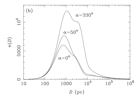
where $R_{\odot}=8000{\mbox{\rm\,\,pc}}$ is the fiducial distance from the Sun to the Galactic centre. The fact that the Sun is actually ‘above’ the Galactic plane with $Z_{\odot}=(24.2\pm 1.7){\mbox{\rm\,\,pc}}$ (Maíz-Apellániz, 2001) is unimportant here as the stellar density varies appreciably only over much greater scales than this. The distribution in $D$, $l$ and $b$ that results from substituting these definitions into Eq. (12) is rather cumbersome, and so not given explicitly here. As argued above, the prior distribution in $l$ and $b$ is unimportant, whereas implied distance distribution has the potential to affect the parameter estimates for a WD, especially given the solid angle degeneracy discussed in Section 1. The distance prior is obtained by multiplying Eq. (12) by the volume element ($\propto D^{2}$) to give

$$\pi(D|l,b)\propto D^{2}\,n_{\mathrm{MS}}\left[R(D,l,b),Z(D,l,b),\Phi(D,l,b)\right],$$ (14)

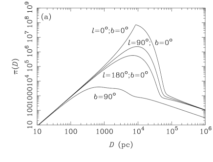
which is shown in in Fig. 2 for several values of $l$ and $b$.

The low-$D$ behaviour is determined by the volume element; beyond $\sim 100{\mbox{\rm\,\,pc}}$ the Galactic direction is more important, with the prior rising steeply towards the Galactic centre, but dropping off sharply when looking out of the plane. In all cases the high-$D$ tail is dominated by the halo component, which is possibly an underestimate for WDs, but which should also fall off faster than this power-law form given in Eq. (12) for $D\ga 10^{5}{\mbox{\rm\,\,pc}}$. A more realistic model would include a sharper fall off in the halo density, but this is irrelevant for the relatively shallow surveys (which can detect WDs only out to $D\simeq 10^{4}{\mbox{\rm\,\,pc}}$) considered here.

One immediate, if somewhat counter-intuitive, implication of the directional dependence of the distance prior is that the parameters inferred for two WDs with identical photometry could be quite different if they are on well separated lines–of–sight. Consider, for example, a very faint WD with measured colours that, if it is assumed to have $\log{\mbox{\em{g}}}\simeq 8$, imply a distance of $D\simeq 10^{4}{\mbox{\rm\,\,pc}}$. Observed towards the Galactic centre this would be completely consistent with prior expectation (cf. the $l=0{\mbox{\rm\,\,deg}}$; $b=0{\mbox{\rm\,\,deg}}$ curve in Fig. 2 a). Observed out of the Galactic plane this would be very surprising, as there are expected to be very few WDs at this distance (which is much greater than the disk scale heights) above or below the Galactic plane, and it would be much more likely that the object is a closer, and correspondingly more massive, WD with $\log{\mbox{\em{g}}}\simeq 9$. Most WDs identified in the current generation of wide-field surveys are closer than this (i.e., local) and so the variation in the Galactic density field is less relevant, but it still has some influence in identifying potential halo WDs.

4.3 Discussion

Whilst the prior given by combining Eqs (10), (11) and (14) is a reasonable approximation to the Galaxy’s WD population, it is incomplete in several ways. The separation of the intrinsic distributions from the positional distribution probably leads to the numbers of thick disk and halo WDs being underestimated (as these stellar populations are older than that of the thin disk). This model is also equivalent to assuming that the different Galactic WD populations have the same age and temperature distributions, which is probably unrealistic, even though there is considerable uncertainty in this area (e.g., Hansen 2001). However these approximations are only important here to the degree that they affect the eventual WD parameter estimates. For photometric data of the quality considered in Section 5 and 6 the most important role of the prior is to encode the fiducial surface gravity value and the relative numbers of thin disk, thick disk and halo WDs, for which Eqs (10) and (14) suffice.

5 Simulations

Figure 3: Marginalised posterior distributions of the model parameters for a simulated WD with $T_{\mathrm{eff}}=10200{\mbox{\rm\,\,K}}$ and $\log{\mbox{\em{g}}}=7.9$ at $D=179{\mbox{\rm\,\,pc}}$, observed in the $g$, $r$, $i$, $z$, $J$, $H$, $K$ bands with photometric noise of $\Delta\hat{m}=0.01$. For both the non-informative prior (grey) and the informative prior (orange) the coloured regions enclose 68 per cent and 95 per cent of the posterior probability in these two parameters. Left: the constraints on the independent model parameters $T_{\mathrm{eff}}$ and $\log{\mbox{\em{g}}}$ are shown, along with the points on the Fontaine–Bergeron model grid (crosses). Right: the degeneracy for black body models (black line) is highlighted by showing constraints on the WD’s distance, $D$, and radius, characterised by $\log{\mbox{\em{g}}}-\log(M/M_{\odot})$. In both panels the true model is indicated by the black spot.

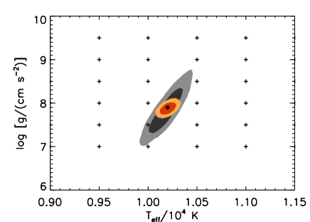
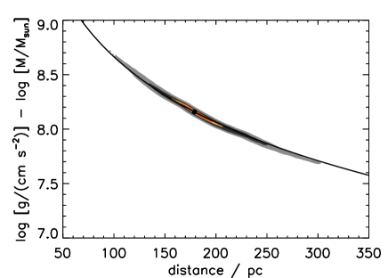
The implication of the parameter inference and model selection methods (described in Sections 2 and 3) for WD surveys can be further understood by applying them to simulated data. A number of representative cases are examined here, although care must be taken in interpreting the Bayesian results obtained using the Galactic WD prior given in Section 4, as the simulated WDs have not been drawn from this distribution.

In each simulation, a surface gravity, $g$, and an effective temperature, $T_{\mathrm{eff}}$, were chosen from within the grid of H atmosphere models provided by Bergeron. This gave absolute AB magnitudes in four SDSS bands ($g$, $r$, $i$ and $z$) and three NIR bands ($J$, $H$ and $K$), which were converted to apparent magnitudes by placing the WD at distance $D$. Finally, photometric noise (of the same level, $\Delta\hat{m}=0.01$, in each band, as appropriate to the SDSS Stripe 82 data) was added to give the simulated data $\hat{\mbox{$g$}}$, $\hat{\mbox{$r$}}$, $\hat{\mbox{$i$}}$, $\hat{\mbox{$z$}}$, $\hat{J}$, $\hat{H}$, and $\hat{K}$. The data were then analysed to give parameter constraints (Section 5.1) and also to test the degree to which H and He WDs could be distinguished (Section 5.2).

5.1 Parameter estimation

WD parameter estimates were obtained from the simulations in several different ways. Both the best-fit model and the best-fit grid value were calculated as described in Section 2.1, and the full posterior distributions of the model parameters were found using the MCMC algorithm outlined in Section 2.2. In the latter case the analysis was performed both with a non-informative prior (uniform in the model parameters) and with the full Galactic WD population prior given in Eq. (9).

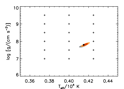
The first case considered is that of a fiducial WD with $\log{\mbox{\em{g}}}=7.9$ and $T_{\mathrm{eff}}=10200{\mbox{\rm\,\,K}}$, results for which are shown in Fig. 3. The most striking feature of this simulation is the strong degeneracy apparent in Fig. 3 (b), which follows the form given in Eq. (1). The temperature is well constrained for both the non-informative and informative priors, although the weak correlation between $T_{\mathrm{eff}}$ and $\log{\mbox{\em{g}}}$ means the constraints are better in the latter case.

This example also illustrates an important point about the identification of outliers, in particular fast-moving halo WDs. If this WD was analysed using the grid-based best-fit method described in Section 2.1, it would be inferred to have ${\log\hat{g}}=7.5$ and $\hat{T}_{\mathrm{eff}}=10000{\mbox{\rm\,\,K}}$, simply because this model grid point is closest to the locus of high likelihood. The resultant distance estimate would be biased, high in this case, by a factor of $\hat{D}/D\simeq 1.2$. The tangential velocity would also be over-estimated, with the possible result that the WD would be identified as a halo object if it had a high proper motion. A more extreme form of this effect explains several of the candidate halo WDs analysed in Section 6.1. It is also an illustration of the general principle that it is no more valid to infer that a WD is dynamically interesting due a large best-fit distance, than it is to infer that the same star is intrinsically unusual by restricting its distance through the application of a prior on its motion. The two possibilities should be balanced by giving the appropriate (not necessarily equal) weight to all the available information.

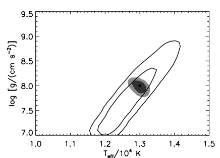
The second example, shown in Fig. 4, is of a $T_{\mathrm{eff}}=10200{\mbox{\rm\,\,K}}$ WD with an unusually high surface gravity of $\log{\mbox{\em{g}}}=8.6$. The results are similar to those for the first example, except for the fact that the true model is well away from the peak of the posterior obtained with the informative prior. This comes about as the prior based on the Galactic distribution of WDs (with $\log{\mbox{\em{g}}}\simeq 8$) is inappropriate to the case of an arbitrarily chosen example. If a real WD was observed to have these colours and the $\log{\mbox{\em{g}}}$ prior given in Eq. (10) is correct, this would be the appropriate inference. In that case the small number of WDs with true colours that match the data would be out-numbered by the fiducial WDs with $\log{\mbox{\em{g}}}\simeq 8$ that were randomly scattered to these observed values.

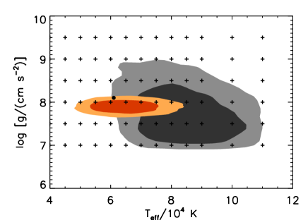
The results for a hot WD with $T_{\mathrm{eff}}=61000{\mbox{\rm\,\,K}}$ and $\log{\mbox{\em{g}}}=8.1$ are shown in Fig. 5. The principal difference here is that the WD’s emission peaks at a wavelength of $\lambda\simeq 0.05{\mbox{\rm\,\,\micron}}$, significantly blueward of the SDSS $g$ band, which has a peak response at $\lambda\simeq 0.5{\mbox{\rm\,\,\micron}}$. As a result it is only the source’s Rayleigh–Jeans tail which is measured, and any temperature of $\ga 6\times 10^{4}{\mbox{\rm\,\,K}}$ is consistent with the data. Both the best-fit analysis and the Bayesian calculation with the non-informative priors give essentially arbitrary parameter estimates, although the latter does at least encode the fact that the uncertainties are large. However when the WD population model from Section 4 is applied, the lower bound on $T_{\mathrm{eff}}$ implied by the data combines with the prior observation that high-$T_{\mathrm{eff}}$ WDs are rare to give a far more precise estimate. This is a particularly good illustration of the equal role that the prior and likelihood have in Bayesian parameter estimation: in isolation they only provide upper and lower bounds, respectively; together they combine the available information to provide the best possible estimate of the WD’s temperature.

Results for the final example, a cool WD with $T_{\mathrm{eff}}=4150{\mbox{\rm\,\,K}}$ and $\log{\mbox{\em{g}}}=7.8$, are shown in Fig. 6. At these temperatures the WD colours have a much greater sensitivity to $g$, and so the data are almost completely informative, with the result that the parameter estimates are insensitive to the nature of the prior, or even to the choice of analysis method. The solid angle degeneracy is still apparent, although the sparsity of the grid (relative to the parameter uncertainties) is such that the best fit from a non-interpolative grid-based search is likely to be outside the formal confidence region in this temperature range.

Figure 4: Same as Fig. 3, but for a simulated WD with $\log{\mbox{\em{g}}}=8.6$ and $T_{\mathrm{eff}}=10200{\mbox{\rm\,\,K}}$ at $D=179{\mbox{\rm\,\,pc}}$.

Figure 5: Same as Fig. 3, but for a simulated WD with $T_{\mathrm{eff}}=61000{\mbox{\rm\,\,K}}$ and $\log{\mbox{\em{g}}}=8.1$ at $D=463{\mbox{\rm\,\,pc}}$.

Figure 6: Same as Fig. 3, but for a simulated WD with $T_{\mathrm{eff}}=4150{\mbox{\rm\,\,K}}$ and $\log{\mbox{\em{g}}}=7.8$ at $D=84{\mbox{\rm\,\,pc}}$.

5.2 Model selection

The model selection techniques described in Section 3.2 can be used in a variety of ways; only one illustrative example is considered here, which is to assess the importance of $u$ band photometry to WD parameter estimation.

As discussed in Section 1, the SDSS Stripe 82 data presented by Ivezić et al. (2007) suggests that per cent level $u$, $g$ and $r$ band photometry should be sufficient to both determine the surface gravity of H atmosphere WDs to reasonable precision, and to distinguish between WDs with H and He atmospheres, at least in the temperature range $10000{\mbox{\rm\,\,K}}\la T_{\mathrm{eff}}\la 18000{\mbox{\rm\,\,K}}$. Both these possibilities were explored quantitatively by simulating observations of a WD with $\log{\mbox{\em{g}}}=8.0$ and $T_{\mathrm{eff}}=13000{\mbox{\rm\,\,K}}$, using the methodology described above, but using all the SDSS bands (i.e., $u$, $g$, $r$, $i$ and $z$).

The results for parameter estimation, obtained with the non-informative priors described in Section 4, are shown in Fig. 7. This confirms that accurate optical and near-UV photometry is sufficient to estimate $\log{\mbox{\em{g}}}$ to within $\sim 0.1$, although a second simulation in only $g$, $r$, $i$ and $z$ also makes it clear that the $u$ band is critical to doing so. The loss of the $u$ band also results in increased uncertainties in $T_{\mathrm{eff}}$ as the remaining bands do not probe the Wien part of the WD’s spectrum as effectively. These points are particularly relevant to the sample of candidate halo WDs analysed by V07 and reanalysed here in Section 6.

Figure 7: Marginalised posterior distributions of the model parameters for a simulated WD with $T_{\mathrm{eff}}=13000{\mbox{\rm\,\,K}}$ and $\log{\mbox{\em{g}}}=8.0$ at $D=200{\mbox{\rm\,\,pc}}$, observed with photometric noise of $\Delta\hat{m}=0.01$ in $u$, $g$, $r$, $i$ and $z$ (shaded contours) and $g$, $r$, $i$ and $z$ only (open contours) The contours enclose 68 per cent and 95 per cent of the posterior probability (obtained using non-informative priors) on the independent model parameters $T_{\mathrm{eff}}$ and $\log{\mbox{\em{g}}}$. The true model is indicated by the black spot.

Given that the separation between the H and He models in Fig. 1 is far greater than that between the various H models with $T_{\mathrm{eff}}\simeq 13000{\mbox{\rm\,\,K}}$, it is clear that photometric data should allow the two classes of models to be distinguished. The evidence, defined in Eq. (5), was calculated for H and He models using the informative priors defined in Eq. (9), both with and without $u$ band data. With $u$ measurements the results are as decisive as expected: $E_{\mathrm{H}}\simeq 0.052$ and $E_{\mathrm{He}}\simeq 0.0$, implying almost no chance that this WD has a He atmosphere, with $P_{\mathrm{He}}\simeq 10^{-5}$. However without the $u$ band data the situation is not quite as clear-cut: $E_{\mathrm{H}}\simeq 7.8$ and $E_{\mathrm{He}}\simeq 1.4$, implying $P_{\mathrm{He}}\simeq 0.02$.

6 Outliers

One of the main utilities of the statistical methods described in Sections 2 and 3 is the assessment and characterisation of putative outliers from the population under consideration. An example of a problem for which this approach is particularly well suited is that of identifying halo WDs. This subject has provoked much debate (e.g., Oppenheimer et al. 2001a; Oppenheimer et al. 2001b; Reid 2005), in part because of the variety of statistical methods used.

One of the largest systematically selected samples of candidate halo objects is that generated by V07, who also identified a number of candidate ultra-cool, and hence potentially old, WDs. These samples were extracted from the SDSS Light–Motion Curve Catalogue (LMCC; Bramich et al. 2008), which provides data for $\sim 4\times 10^{6}$ sources in SDSS Stripe 82 that were observed at $\sim 20$ different epochs spanning $\sim 7{\mbox{\rm\,\,yr}}$. As such, the LMCC has improved astrometry and photometry relative to the main SDSS survey, with uncertainties of $\Delta\hat{\mu}\simeq 5{\mbox{\rm\,\,milliarcsec}}{\mbox{\rm\,\,yr}}^{-1}$ and $\Delta\hat{\mbox{$r$}}\simeq 0.01$ at $\hat{\mbox{$r$}}\simeq 20$. The photometry in the $g$, $i$ and $z$ bands is of similar quality, although there were fewer good $u$ band observations, necessitating the exclusion of the $u$ band from the V07 analysis, a significant loss in the context of WD studies (cf. Section 5.2). V07 were able to produce an exquisite reduced proper motion (RPM) diagram in which the WD population was very clearly separated from the MS stars, and the resultant sample of 1049 WDs is probably contaminated at no more than the $\sim 2$ per cent level (cf. Kilic et al. 2006; Harris et al. 2006).

V07 then cross-matched the WD sample with the UKIRT Infrared Deep Sky Survey (UKIDSS; Lawrence et al. 2007), which yielded $Y$, $J$, $H$ and $K$ band photometry for about half the sources (as the UKIDSS observations in Stripe 82 were only partially complete at the time). The addition of NIR photometry is particularly valuable in the analysis of the coolest WDs due to the observed depleted flux at these wavelengths (Hodgkin et al., 2000), although the $Y$ band data were not used by V07 as the Fontaine–Bergeron model grids do not include this filter.

The next stage in V07’s analysis was to estimate the WDs’ parameters from the stacked $g$, $r$, $i$ and $z$ band SDSS photometry and, where available, the $J$, $H$ and $K$ UKIDSS measurements. This was done by finding the best fit from a discrete set of models defined by combining the Fontaine–Bergeron grid with a uniform sampling (multiples of $5{\mbox{\rm\,\,pc}}$) in distance. This yielded parameter estimates ${\log\hat{g}}$, $\hat{T}_{\mathrm{eff}}$ and $\hat{D}$ which, when combined with the observed proper motion, $\hat{\mu}$, yielded a tangential velocity estimate of ${\hat{V}_{\mathrm{tan}}}=\hat{D}\hat{\mu}$. Uncertainties were characterised by finding the location of the second-best fitting grid point, although these values were not explicitly reported. V07 then identified 34 candidate halo WDs with estimated tangential velocities of ${\hat{V}_{\mathrm{tan}}}\geq 160{\mbox{\rm\,\,km}}{\mbox{\rm\,\,s}}^{-1}$, as well as 24 candidate ultra-cool WDs with best-fit temperatures of $\hat{T}_{\mathrm{eff}}\leq 4000{\mbox{\rm\,\,K}}$. V07 took care to point out some of the systematic effects, including the solid angle degeneracy, that might affect the candidate selection, and one of the motivations for this reanalysis is to quantify some of these biases.

6.1 Candidate halo white dwarfs

Table 1: Estimated H atmosphere model parameters of the 34 V07 candidate halo WDs, obtained using the informative prior defined in Eq. (9).

object	$T_{\mathrm{eff}}$	$\log{\mbox{\em{g}}}$	$M$	$T$	$D$	$V_{\mathrm{tan}}$
	(K)		$(M_{\odot})$	(yr)	(pc)	(km s-1)
SDSS J000244.03$+$010945.8	$(1.11\pm 0.02)\times 10^{4}$	$7.88\pm 0.10$	$0.55\pm 0.05$	$(4.04\pm 0.39)\times 10^{8}$	$453\pm 25$	$110\pm 12$
SDSS J000557.24$+$001833.2	$(9.01\pm 0.08)\times 10^{3}$	$7.89\pm 0.10$	$0.54\pm 0.05$	$(7.06\pm 0.68)\times 10^{8}$	$179\pm 10$	$178\pm 11$
SDSS J001306.23$+$005506.4	$(1.05\pm 0.01)\times 10^{4}$	$7.88\pm 0.10$	$0.54\pm 0.05$	$(4.63\pm 0.43)\times 10^{8}$	$318\pm 18$	$158\pm 11$
SDSS J001518.33$+$010549.2	$(1.24\pm 0.03)\times 10^{4}$	$7.86\pm 0.10$	$0.54\pm 0.05$	$(2.91\pm 0.29)\times 10^{8}$	$483\pm 26$	$158\pm 14$
SDSS J001838.54$+$005943.5	$(1.83\pm 0.06)\times 10^{4}$	$7.87\pm 0.10$	$0.56\pm 0.05$	$(8.24\pm 1.27)\times 10^{7}$	$623\pm 38$	$100\pm 16$
SDSS J002951.64$+$005623.6	$(1.17\pm 0.02)\times 10^{4}$	$7.88\pm 0.10$	$0.55\pm 0.05$	$(3.50\pm 0.35)\times 10^{8}$	$553\pm 31$	$228\pm 20$
SDSS J003054.06$+$001115.6	$(7.93\pm 0.08)\times 10^{3}$	$7.89\pm 0.10$	$0.54\pm 0.05$	$(9.93\pm 1.04)\times 10^{8}$	$353\pm 21$	$160\pm 17$
SDSS J003730.58$-$001657.8	$(8.85\pm 0.10)\times 10^{3}$	$7.89\pm 0.09$	$0.54\pm 0.05$	$(7.46\pm 0.72)\times 10^{8}$	$304\pm 18$	$108\pm 10$
SDSS J003813.53$-$000128.8	$(1.21\pm 0.02)\times 10^{4}$	$7.87\pm 0.10$	$0.55\pm 0.05$	$(3.17\pm 0.31)\times 10^{8}$	$310\pm 17$	$220\pm 13$
SDSS J004214.88$+$001135.7	$(1.23\pm 0.03)\times 10^{4}$	$7.88\pm 0.10$	$0.55\pm 0.05$	$(3.09\pm 0.30)\times 10^{8}$	$496\pm 27$	$115\pm 13$
SDSS J005906.78$+$001725.2	$(1.07\pm 0.01)\times 10^{4}$	$7.88\pm 0.10$	$0.54\pm 0.05$	$(4.48\pm 0.42)\times 10^{8}$	$294\pm 16$	$143\pm 10$
SDSS J010129.81$-$003041.7	$(1.28\pm 0.03)\times 10^{4}$	$7.88\pm 0.10$	$0.55\pm 0.05$	$(2.76\pm 0.28)\times 10^{8}$	$565\pm 31$	$107\pm 15$
SDSS J010207.24$-$003259.7	$(1.08\pm 0.01)\times 10^{4}$	$7.89\pm 0.10$	$0.55\pm 0.05$	$(4.40\pm 0.41)\times 10^{8}$	$191\pm 11$	$334\pm 19$
SDSS J010225.13$-$005458.4	$(1.43\pm 0.03)\times 10^{4}$	$7.88\pm 0.10$	$0.56\pm 0.05$	$(1.97\pm 0.22)\times 10^{8}$	$429\pm 24$	$216\pm 15$
SDSS J014247.10$+$005228.4	$(1.27\pm 0.02)\times 10^{4}$	$7.87\pm 0.10$	$0.55\pm 0.05$	$(2.81\pm 0.28)\times 10^{8}$	$408\pm 22$	$114\pm 10$
SDSS J015227.57$-$002421.1	$(9.21\pm 0.11)\times 10^{3}$	$7.89\pm 0.10$	$0.54\pm 0.05$	$(6.69\pm 0.65)\times 10^{8}$	$351\pm 21$	$118\pm 11$
SDSS J020241.81$-$005743.0	$(7.59\pm 0.07)\times 10^{3}$	$7.89\pm 0.10$	$0.54\pm 0.05$	$(1.10\pm 0.11)\times 10^{9}$	$226\pm 13$	$113\pm 8$
SDSS J020729.85$+$000637.6	$(5.64\pm 0.03)\times 10^{3}$	$7.88\pm 0.10$	$0.53\pm 0.05$	$(2.50\pm 0.31)\times 10^{9}$	$163\pm 9$	$115\pm 8$
SDSS J024529.69$-$004229.8	$(1.42\pm 0.03)\times 10^{4}$	$7.87\pm 0.10$	$0.55\pm 0.05$	$(1.98\pm 0.22)\times 10^{8}$	$568\pm 32$	$137\pm 13$
SDSS J024837.53$-$003123.9	$(8.80\pm 0.07)\times 10^{3}$	$7.89\pm 0.10$	$0.54\pm 0.05$	$(7.54\pm 0.73)\times 10^{8}$	$216\pm 13$	$328\pm 20$
SDSS J025325.83$-$002751.5	$(1.43\pm 0.03)\times 10^{4}$	$7.80\pm 0.10$	$0.52\pm 0.05$	$(1.77\pm 0.20)\times 10^{8}$	$265\pm 15$	$125\pm 8$
SDSS J025531.00$-$005552.8	$(1.13\pm 0.02)\times 10^{4}$	$7.88\pm 0.10$	$0.55\pm 0.05$	$(3.88\pm 0.38)\times 10^{8}$	$448\pm 25$	$149\pm 12$
SDSS J030433.61$-$002733.2	$(6.46\pm 0.05)\times 10^{3}$	$7.89\pm 0.10$	$0.54\pm 0.05$	$(1.65\pm 0.18)\times 10^{9}$	$283\pm 16$	$130\pm 12$
SDSS J211928.44$-$002632.9	$(1.52\pm 0.04)\times 10^{4}$	$7.87\pm 0.10$	$0.55\pm 0.05$	$(1.60\pm 0.20)\times 10^{8}$	$461\pm 27$	$103\pm 12$
SDSS J213641.39$+$010504.9	$(1.16\pm 0.02)\times 10^{4}$	$7.88\pm 0.10$	$0.55\pm 0.05$	$(3.55\pm 0.34)\times 10^{8}$	$454\pm 25$	$97\pm 14$
SDSS J215138.09$+$003222.3	$(7.22\pm 0.06)\times 10^{3}$	$7.89\pm 0.10$	$0.54\pm 0.05$	$(1.26\pm 0.13)\times 10^{9}$	$247\pm 15$	$124\pm 10$
SDSS J223808.18$+$003247.9	$(6.53\pm 0.05)\times 10^{3}$	$7.88\pm 0.10$	$0.53\pm 0.05$	$(1.59\pm 0.18)\times 10^{9}$	$213\pm 12$	$289\pm 18$
SDSS J223815.97$-$011336.9	$(7.61\pm 0.07)\times 10^{3}$	$7.88\pm 0.10$	$0.53\pm 0.05$	$(1.08\pm 0.11)\times 10^{9}$	$328\pm 20$	$110\pm 13$
SDSS J230534.79$-$010225.2	$(1.04\pm 0.01)\times 10^{4}$	$7.89\pm 0.10$	$0.55\pm 0.05$	$(4.88\pm 0.46)\times 10^{8}$	$431\pm 24$	$145\pm 13$
SDSS J231626.98$+$004607.0	$(4.88\pm 0.03)\times 10^{3}$	$7.89\pm 0.10$	$0.52\pm 0.05$	$(4.99\pm 0.94)\times 10^{9}$	$130\pm 7$	$100\pm 6$
SDSS J233227.63$-$010713.8	$(1.18\pm 0.02)\times 10^{4}$	$7.88\pm 0.10$	$0.55\pm 0.05$	$(3.47\pm 0.34)\times 10^{8}$	$379\pm 21$	$97\pm 9$
SDSS J233817.06$-$005720.1	$(9.75\pm 0.12)\times 10^{3}$	$7.88\pm 0.10$	$0.54\pm 0.05$	$(5.75\pm 0.55)\times 10^{8}$	$440\pm 26$	$177\pm 16$
SDSS J234110.13$+$003259.5	$(1.21\pm 0.02)\times 10^{4}$	$7.87\pm 0.10$	$0.54\pm 0.05$	$(3.18\pm 0.32)\times 10^{8}$	$342\pm 19$	$177\pm 12$
SDSS J235138.85$+$002716.9	$(7.08\pm 0.06)\times 10^{3}$	$7.89\pm 0.10$	$0.54\pm 0.05$	$(1.32\pm 0.14)\times 10^{9}$	$321\pm 19$	$146\pm 15$

Table 2: Estimated He atmosphere model parameters of the 34 V07 candidate halo WDs, obtained using the informative prior defined in Eq. (9).

object	$T_{\mathrm{eff}}$	$\log{\mbox{\em{g}}}$	$M$	$T$	$D$	$V_{\mathrm{tan}}$
	(K)		$(M_{\odot})$	(yr)	(pc)	(km s-1)
SDSS J000244.03$+$010945.8	$(1.12\pm 0.02)\times 10^{4}$	$7.89\pm 0.10$	$0.53\pm 0.05$	$(4.29\pm 0.52)\times 10^{8}$	$436\pm 27$	$105\pm 12$
SDSS J000557.24$+$001833.2	$(8.87\pm 0.08)\times 10^{3}$	$7.89\pm 0.10$	$0.53\pm 0.05$	$(8.02\pm 0.94)\times 10^{8}$	$172\pm 10$	$171\pm 11$
SDSS J001306.23$+$005506.4	$(1.07\pm 0.01)\times 10^{4}$	$7.89\pm 0.10$	$0.53\pm 0.05$	$(4.92\pm 0.59)\times 10^{8}$	$306\pm 19$	$152\pm 11$
SDSS J001518.33$+$010549.2	$(1.27\pm 0.02)\times 10^{4}$	$7.89\pm 0.10$	$0.54\pm 0.05$	$(3.09\pm 0.40)\times 10^{8}$	$472\pm 30$	$154\pm 15$
SDSS J001838.54$+$005943.5	$(1.96\pm 0.07)\times 10^{4}$	$7.90\pm 0.10$	$0.55\pm 0.04$	$(7.42\pm 1.31)\times 10^{7}$	$678\pm 44$	$109\pm 18$
SDSS J002951.64$+$005623.6	$(1.19\pm 0.02)\times 10^{4}$	$7.89\pm 0.10$	$0.54\pm 0.05$	$(3.69\pm 0.47)\times 10^{8}$	$535\pm 34$	$221\pm 21$
SDSS J003054.06$+$001115.6	$(7.84\pm 0.08)\times 10^{3}$	$7.90\pm 0.10$	$0.53\pm 0.05$	$(1.11\pm 0.14)\times 10^{9}$	$349\pm 21$	$159\pm 16$
SDSS J003730.58$-$001657.8	$(8.75\pm 0.10)\times 10^{3}$	$7.89\pm 0.10$	$0.53\pm 0.05$	$(8.34\pm 0.99)\times 10^{8}$	$297\pm 18$	$106\pm 9$
SDSS J003813.53$-$000128.8	$(1.25\pm 0.02)\times 10^{4}$	$7.89\pm 0.10$	$0.53\pm 0.05$	$(3.18\pm 0.40)\times 10^{8}$	$308\pm 19$	$219\pm 15$
SDSS J004214.88$+$001135.7	$(1.24\pm 0.02)\times 10^{4}$	$7.89\pm 0.10$	$0.53\pm 0.05$	$(3.25\pm 0.43)\times 10^{8}$	$486\pm 31$	$113\pm 14$
SDSS J005906.78$+$001725.2	$(1.08\pm 0.01)\times 10^{4}$	$7.89\pm 0.10$	$0.53\pm 0.05$	$(4.73\pm 0.57)\times 10^{8}$	$284\pm 18$	$138\pm 10$
SDSS J010129.81$-$003041.7	$(1.29\pm 0.02)\times 10^{4}$	$7.89\pm 0.10$	$0.54\pm 0.05$	$(2.91\pm 0.39)\times 10^{8}$	$559\pm 35$	$106\pm 15$
SDSS J010207.24$-$003259.7	$(1.10\pm 0.01)\times 10^{4}$	$7.89\pm 0.10$	$0.53\pm 0.05$	$(4.54\pm 0.54)\times 10^{8}$	$186\pm 11$	$327\pm 20$
SDSS J010225.13$-$005458.4	$(1.47\pm 0.03)\times 10^{4}$	$7.89\pm 0.10$	$0.54\pm 0.05$	$(1.97\pm 0.29)\times 10^{8}$	$442\pm 29$	$222\pm 17$
SDSS J014247.10$+$005228.4	$(1.29\pm 0.02)\times 10^{4}$	$7.89\pm 0.10$	$0.54\pm 0.05$	$(2.91\pm 0.38)\times 10^{8}$	$405\pm 25$	$113\pm 10$
SDSS J015227.57$-$002421.1	$(9.13\pm 0.11)\times 10^{3}$	$7.89\pm 0.10$	$0.53\pm 0.05$	$(7.46\pm 0.88)\times 10^{8}$	$340\pm 21$	$115\pm 11$
SDSS J020241.81$-$005743.0	$(7.46\pm 0.06)\times 10^{3}$	$7.89\pm 0.10$	$0.52\pm 0.05$	$(1.25\pm 0.15)\times 10^{9}$	$222\pm 13$	$112\pm 8$
SDSS J020729.85$+$000637.6	$(5.67\pm 0.03)\times 10^{3}$	$7.93\pm 0.10$	$0.54\pm 0.05$	$(3.06\pm 0.46)\times 10^{9}$	$164\pm 10$	$116\pm 8$
SDSS J024529.69$-$004229.8	$(1.45\pm 0.03)\times 10^{4}$	$7.90\pm 0.10$	$0.54\pm 0.05$	$(2.08\pm 0.30)\times 10^{8}$	$573\pm 37$	$139\pm 14$
SDSS J024837.53$-$003123.9	$(8.67\pm 0.08)\times 10^{3}$	$7.90\pm 0.09$	$0.53\pm 0.05$	$(8.67\pm 1.01)\times 10^{8}$	$208\pm 12$	$316\pm 19$
SDSS J025325.83$-$002751.5	$(1.49\pm 0.03)\times 10^{4}$	$7.89\pm 0.10$	$0.54\pm 0.05$	$(1.88\pm 0.27)\times 10^{8}$	$263\pm 17$	$125\pm 9$
SDSS J025531.00$-$005552.8	$(1.14\pm 0.02)\times 10^{4}$	$7.89\pm 0.10$	$0.53\pm 0.05$	$(4.09\pm 0.50)\times 10^{8}$	$432\pm 27$	$143\pm 12$
SDSS J030433.61$-$002733.2	$(6.40\pm 0.04)\times 10^{3}$	$7.91\pm 0.10$	$0.53\pm 0.05$	$(1.88\pm 0.24)\times 10^{9}$	$280\pm 17$	$129\pm 12$
SDSS J211928.44$-$002632.9	$(1.56\pm 0.04)\times 10^{4}$	$7.90\pm 0.10$	$0.55\pm 0.05$	$(1.64\pm 0.25)\times 10^{8}$	$474\pm 32$	$106\pm 13$
SDSS J213641.39$+$010504.9	$(1.18\pm 0.02)\times 10^{4}$	$7.89\pm 0.10$	$0.53\pm 0.05$	$(3.75\pm 0.47)\times 10^{8}$	$438\pm 28$	$94\pm 14$
SDSS J215138.09$+$003222.3	$(7.12\pm 0.06)\times 10^{3}$	$7.90\pm 0.10$	$0.53\pm 0.05$	$(1.41\pm 0.17)\times 10^{9}$	$244\pm 15$	$123\pm 10$
SDSS J223808.18$+$003247.9	$(6.43\pm 0.04)\times 10^{3}$	$7.93\pm 0.10$	$0.54\pm 0.05$	$(1.89\pm 0.24)\times 10^{9}$	$206\pm 12$	$279\pm 18$
SDSS J223815.97$-$011336.9	$(7.53\pm 0.07)\times 10^{3}$	$7.89\pm 0.10$	$0.52\pm 0.05$	$(1.21\pm 0.15)\times 10^{9}$	$325\pm 19$	$109\pm 13$
SDSS J230534.79$-$010225.2	$(1.04\pm 0.02)\times 10^{4}$	$7.89\pm 0.10$	$0.53\pm 0.05$	$(5.27\pm 0.63)\times 10^{8}$	$413\pm 25$	$139\pm 13$
SDSS J231626.98$+$004607.0	$(5.13\pm 0.02)\times 10^{3}$	$7.90\pm 0.10$	$0.52\pm 0.05$	$(4.59\pm 0.81)\times 10^{9}$	$148\pm 9$	$114\pm 8$
SDSS J233227.63$-$010713.8	$(1.20\pm 0.02)\times 10^{4}$	$7.89\pm 0.10$	$0.53\pm 0.05$	$(3.58\pm 0.45)\times 10^{8}$	$371\pm 23$	$95\pm 9$
SDSS J233817.06$-$005720.1	$(9.74\pm 0.12)\times 10^{3}$	$7.89\pm 0.10$	$0.53\pm 0.05$	$(6.30\pm 0.74)\times 10^{8}$	$424\pm 26$	$171\pm 16$
SDSS J234110.13$+$003259.5	$(1.23\pm 0.02)\times 10^{4}$	$7.89\pm 0.10$	$0.53\pm 0.05$	$(3.30\pm 0.42)\times 10^{8}$	$334\pm 21$	$173\pm 12$
SDSS J235138.85$+$002716.9	$(7.00\pm 0.06)\times 10^{3}$	$7.89\pm 0.10$	$0.52\pm 0.05$	$(1.46\pm 0.18)\times 10^{9}$	$319\pm 19$	$145\pm 15$

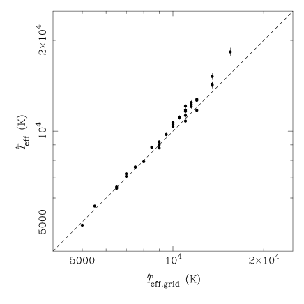
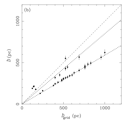
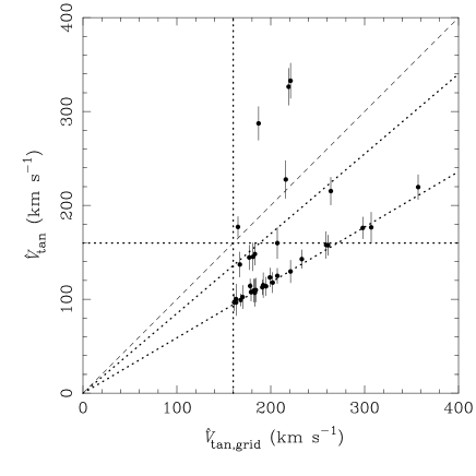
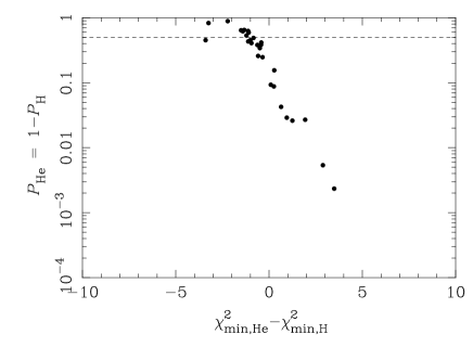
The 34 candidate halo WDs identified by V07 were reanalysed using the Bayesian techniques described in Sections 2 and 3, giving parameter estimates and evidence values for both H and He atmosphere models, and for both the non-informative and informative priors defined in Section 4. The results are presented in Tables 1 and 2. The Bayesian parameter fits are compared to those obtained by V07 in Figs. 8, 9 and 10. The model comparison results, used to distinguish between the H and He models, are presented in Fig. 11.

Fig. 8 shows the expected result that the Bayesian effective temperature estimates match those of V07. The estimates are insensitive to the prior, as the well-measured SDSS (and UKIDSS) colours unambiguously constrain $T_{\mathrm{eff}}$. If the data are sufficiently informative then the details of the parameter estimation method are secondary, and that is the situation here. The clear agreement between the two estimates notwithstanding, the Bayesian values are systematically higher; this is an artefact of the much stronger distance bias discussed below, which has a small effect here because there is a slight anti-correlation between $\hat{T}_{\mathrm{eff}}$ and $\hat{D}$ for WDs with $T_{\mathrm{eff}}\simeq 10^{4}{\mbox{\rm\,\,K}}$.

Figure 8: The estimated effective temperature, $\hat{T}_{\mathrm{eff}}$, of the 34 candidate halo WDs as found by V07, and using the Bayesian methods described here (for the H atmosphere models with the Galactic model priors).

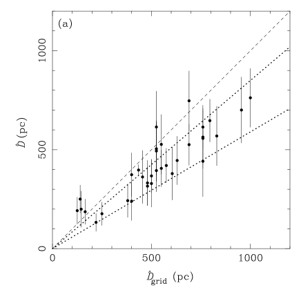
The Bayesian distance estimates for the halo candidates differ considerably from those given by V07, as can be seen from Fig. 9. For both the non-informative and informative priors the Bayesian estimates are lower, for what turn out to be related (but distinct) reasons.

In the case of non-informative priors it is because the V07 parameter search is performed on a discrete grid of models. The grid point with the lowest $\chi^{2}$ is unlikely to be the true best-fit, even if it might be close. In many problems this would merely result in a small error in the parameter estimates on a scale comparable to the grid spacing. However, the strong degeneracy in the WD models exacerbates this problem, as the locus of models with good fits can ‘thread’ the model grid, as shown in Figs. 3, 4 and 6. This explains why the grid-based estimates can differ significantly from the true best fit distance, but not why they are systematically higher. The bias seen in Fig. 9 can be traced back to the fact that the 34 candidate halo WDs were not selected randomly, but by virtue of having large ${\hat{V}_{\mathrm{tan}}}$ and hence high $\hat{D}$. Thus WDs for which the error due to the grid-based fitting randomly leads to an over-estimate of $D$ will preferentially be selected into a sample of objects with high inferred tangential velocities, explaining the observed bias.

The difference between the Bayesian distance estimates obtained using the informative prior and those of V07 are even greater, as shown in Fig. 9 (b). The selection bias described above is still present, but the strongly peaked $\log{\mbox{\em{g}}}$ prior given in Eq. (10) is the dominant factor. With all the models along the degeneracy being comparably good fits to the data, the informative prior results in the posterior being strongly peaked at, in this case, $\log{\mbox{\em{g}}}\simeq 7.9$. This effectively breaks the degeneracy, and the tight limits on $\log{\mbox{\em{g}}}$ from the prior then translate into a comparably tight constraint on $D$. The obvious locus of points with $\hat{D}\simeq 0.6\,\hat{D}_{\mathrm{grid}}$ are those for which the best fit grid point has ${\log\hat{g}}=7.0$ and the Bayesian models have the prior-selected value of $\log{\mbox{\em{g}}}\simeq 7.9$; the distance ratio implied by Eq. (1) is $0.59$. There are also a few points with $\hat{D}\simeq 0.85\,\hat{D}_{\mathrm{grid}}$; these are the WDs for which the best-fit grid point has ${\log\hat{g}}=7.5$. Whilst it is not necessarily unexpected that a warm, and hence young, halo WD would have low mass and $\log{\mbox{\em{g}}}$, such objects are expected to extremely rare. A more probable explanation is that these are members of the much greater thin disk and thick disk populations for which the grid-based fitting procedures happened to yield the the twin abnormalities of high $\hat{D}$ and low ${\log\hat{g}}$. (For a more detailed discussion of this idea see Section 6.1.1.) The tightness of the loci in Fig. 9 is also rather striking, and suggests that the informative $\log{\mbox{\em{g}}}$ prior defined in Eq. (10) is overly prescriptive; the true $\log{\mbox{\em{g}}}$ distribution almost certainly has broader, non-Gaussian wings, and the resultant distance estimates probably should lie between the two extremes presented here.

Figure 9: The estimated distance, $\hat{D}$, to the 34 candidate halo WDs as calculated by V07 and obtained using the Bayesian method described here [for H atmosphere models, with the non-informative priors in (a) and the Galactic model priors in (b)]. The two dotted lines show the loci $\hat{D}=0.6\,\hat{D}_{\mathrm{grid}}$ and $\hat{D}=0.85\,\hat{D}_{\mathrm{grid}}$, expected for WDs with unconstrained surface gravities for which V07 estimate ${\log\hat{g}}=7.0$ and ${\log\hat{g}}=7.5$, respectively.

The estimated tangential velocity, ${\hat{V}_{\mathrm{tan}}}$, is directly related to the distance estimates described above by ${\hat{V}_{\mathrm{tan}}}=\hat{D}\hat{\mu}$, and so it is not surprising that Fig. 10 exhibits some of the same features as Fig. 9. In particular the Bayesian values of ${\hat{V}_{\mathrm{tan}}}$ are correspondingly smaller than those given by V07, and only 10 of these 34 sources would satisfy the $V_{\mathrm{tan}}\geq 160{\mbox{\rm\,\,km}}{\mbox{\rm\,\,s}}^{-1}$ criterion as candidate halo WDs if the Bayesian estimates were used. Just as before, the Gaussian $\log{\mbox{\em{g}}}$ prior is probably overly prescriptive, but the essential conclusion, that the tangential velocities of these objects are lower than estimated by V07, is fairly robust. There are also three WDs, discussed further in Section 6.1.1, for which the Bayesian estimate of $V_{\mathrm{tan}}$ is considerably greater than that quoted by V07. They also have the three highest measured proper motions of the 34 WDs in the sample, which reinforces their identification as halo candidates. Their measured proper motions also give some information about their direction of motion, which could in principle constrain them to have low $D$, most obviously if this implied an unreasonably high orbital speed along the Solar circle. However this is not the case for any of these three sources, and the uncertainty due to the lack of radial velocity information makes it difficult to say more.

The best way to include this dynamical information would be to adopt a velocity prior, in much the same way as the distance prior was developed in Section 4.2. As changing the distance to a WD with fixed physical properties and a fixed spatial velocity, ${V}$, would affect both its measured photometry and proper motion, it is the only way to correctly include the available prior information (i.e., on $g$, $T_{\mathrm{eff}}$, $D$ and ${V}$) and thus utilise all the available data simultaneously (cf. Hogg et al. 2005).

Figure 10: The estimated tangential velocity, ${\hat{V}_{\mathrm{tan}}}$, of the 34 candidate halo WDs as found by V07 and obtained using the Bayesian method described here (for H atmosphere models, with the Galactic model priors). The horizontal and vertical dotted lines show the criterion of $V_{\mathrm{tan}}\geq 160{\mbox{\rm\,\,km}}{\mbox{\rm\,\,s}}^{-1}$ used by V07 to select their sample of halo candidates. The other two dotted lines show the loci ${\hat{V}_{\mathrm{tan}}}=0.6\,{\hat{V}_{\mathrm{tan,grid}}}$ and ${\hat{V}_{\mathrm{tan}}}=0.85\,{\hat{V}_{\mathrm{tan,grid}}}$, expected for WDs with unconstrained surface gravities for which V07 estimate $\log{\mbox{\em{g}}}=7.0$ and $\log{\mbox{\em{g}}}=7.5$, respectively.

All the above results were obtained under the assumption that the V07 halo candidates have H atmospheres, but given that $\sim 10$ per cent of WDs have He atmospheres, several of the 34 halo candidates are probably in this category. This can be assessed objectively by using the model comparison formalism described in Section 3. Comparing $E_{\mathrm{H}}$ and $E_{\mathrm{He}}$ reveals that most of the 34 halo candidates are reasonably consistent with either model, with $|\ln(E_{\mathrm{H}})-\ln(E_{\mathrm{He}})|\la 5$, although some are decisively better fits to the H models. However, care must be taken in interpreting the evidence, as its numerical value itself is of little meaning in isolation, especially due to the strong model prior that H atmosphere WDs are so more common than He WDs. Adopting the model prior $\pi_{\mathrm{H}}=0.9$ (discussed in Section 4) allows the posterior model probability, $P_{\mathrm{H}}$, to be calculated according to Eq. (8). These are shown in Fig. 11 and compared to the commonly used model comparison statistic $\Delta\chi^{2}=\chi^{2}_{{\mathrm{min}},{\mathrm{He}}}-\chi^{2}_{{\mathrm{min}},{\mathrm{H}}}$ (cf. Section 3). As expected, this is correlated with $P_{\mathrm{H}}$, but there is a broad scatter in this relation because $\Delta\chi^{2}$ is sensitive only to a single point in parameter space (i.e., the best fit) whereas $P_{\mathrm{H}}$ is a properly weighted integral over all the possible models. There is also a systematic shift due to the strong model prior; if it was set to the non-informative value of $\pi_{\mathrm{H}}=0.5$, all the points would be higher in Fig. 11 and the more probable hypothesis would be simply that with the higher evidence value, as seen from Eq. (8).

Figure 11: A comparison of the H and He fits to the 34 candidate halo WDs. The difference in $\chi^{2}_{\mathrm{min}}$ is compared to the Bayesian probability that the WD has a H atmosphere, $P_{\mathrm{H}}$, calculated assuming the prior probability that any WD has a H atmosphere is $\pi_{\mathrm{H}}=0.9$. The dashed horizontal line is located at $P_{\mathrm{H}}=P_{\mathrm{He}}=0.5$; the eight WDs above this line probably have He atmospheres, though in no case is this conclusion decisive. Each star in the subset of the probable He stars for which spectroscopic confirmation exists in the Eisenstein et al. (2006) sample has been classified as type DA.

In order to investigate these conclusions further, Table 4 gives some of the quantities used in model selection. The best fit $\log{\mbox{\em{g}}}$ obtained with the uninformative $\log{\mbox{\em{g}}}$ prior is shown as a proxy for the influence of the informative $\log{\mbox{\em{g}}}$ prior – the further this is from $\log{\mbox{\em{g}}}=7.9$, the stronger the effect of the $g$ prior will be in the model selection. The best fit $\chi^{2}$ (for the uninformative prior) is shown as an indicator of the influence of the data. The evidence values are presented to indicate how consistent the data are with each model over the entire model space. If neither the $g$ prior nor the data definitively picks out an atmosphere model, the 10:1 model prior dominates the model selection. Finally, the probability of the WD having a H atmosphere is listed, along with an indication of the driving force behind this conclusion.

Table 3: Estimated model parameters of the 17 V07 candidate halo WDs with spectroscopic fits presented by Eisenstein et al. (2006). Three WDs, SDSS J024837.53$-$003123.9, SDSS J024837.53$-$003123.9 and SDSS J234110.13$+$003259.5, were observed twice.

object	type	${\log\hat{g}}$	$\hat{T}_{\mathrm{eff}}$
			(K)
SDSS J000557.24$+$001833.2	DZ	$7.78\pm 0.58$	$10110\pm 50$
SDSS J001306.23$+$005506.4	DA	$8.13\pm 0.14$	$10890\pm 170$
SDSS J001838.54$+$005943.5	DA	$7.64\pm 0.13$	$21820\pm 760$
SDSS J003730.58$-$001657.8	DA	$7.93\pm 0.38$	$9130\pm 160$
SDSS J003813.53$-$000128.8	DA	$8.03\pm 0.11$	$12140\pm 400$
SDSS J005906.78$+$001725.2	DZ	$8.53\pm 0.38$	$11180\pm 270$
SDSS J010207.24$-$003259.7	DA	$8.24\pm 0.08$	$11050\pm 100$
SDSS J010225.13$-$005458.4	DA	$8.95\pm 0.06$	$18790\pm 830$
SDSS J014247.10$+$005228.4	DA	$8.82\pm 0.11$	$14040\pm 450$
SDSS J024837.53$-$003123.9	DA	$7.81\pm 0.15$	$9080\pm 80$
	DA	$8.11\pm 0.17$	$9500\pm 110$
SDSS J025325.83$-$002751.5	DA	$7.70\pm 0.03$	$19200\pm 200$
SDSS J025531.00$-$005552.8	DA	$7.72\pm 0.20$	$12720\pm 640$
	DA	$7.74\pm 0.15$	$12830\pm 440$
SDSS J211928.44$-$002632.9	DA	$7.87\pm 0.10$	$15660\pm 410$
SDSS J215138.09$+$003222.3	DA	$8.23\pm 0.45$	$7820\pm 210$
SDSS J233227.63$-$010713.8	DA	$7.60\pm 0.20$	$14420\pm 1320$
SDSS J233817.06$-$005720.1	DA	$8.07\pm 0.33$	$10380\pm 280$
SDSS J234110.13$+$003259.5	DA	$7.90\pm 0.08$	$13380\pm 330$
	DA	$7.80\pm 0.09$	$12830\pm 280$

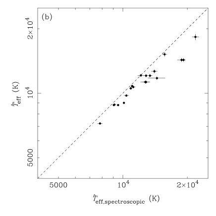
Overall, the implication of these results is that many of the candidate halo stars do not actually have the high tangential velocities that the data seem to imply. This hypothesis could be tested by obtaining follow-up observations, although higher precision photometry (other than $u$ band) would be of little use, as the ambiguities are dominated by the fundamental WD model degeneracies, not the quality of the existing photometry. Distances based on parallaxes would obviously be definitive, but impractical with current observational resources. That leaves spectroscopic follow-up, although in many cases this is not necessary as 17 of the 34 halo candidates already have spectroscopic fits presented by Eisenstein et al. (2006). These spectroscopic fits (only $\log{\mbox{\em{g}}}$ and $T_{\mathrm{eff}}$, but not $D$) are given in Table 3, and compared to the Bayesian estimates of $T_{\mathrm{eff}}$ in Fig. 12.

Table 4: Model selection quantities for the 34 V07 candidate halo WDs, where columns 2 and 3 are the best-fit $\log{\mbox{\em{g}}}$ values estimated using the uninformative $g$ prior. UKIDSS data have been used where available. The final column states whether the model selection result is driven by the data, the informative $g$ prior, or the 10:1 model prior.

object	$\log g_{\mathrm{H}}$	$\log g_{\mathrm{He}}$	$\chi^{2}_{\rm min,{\mathrm{H}}}$	$\chi^{2}_{\rm min,{\mathrm{He}}}$	$E_{\mathrm{H}}$	$E_{\mathrm{He}}$	$P_{\mathrm{H}}$	notes
SDSS J000244.03$+$010945.8	7.57	7.83	16.5	14.1	$1.2\times 10^{-02}$	$1.2\times 10^{-01}$	$0.47$	data and $g$ prior
SDSS J000557.24$+$001833.2	7.86	7.89	2.8	4.1	$5.6\times 10^{-02}$	$2.3\times 10^{-02}$	$0.96$	data and model prior
SDSS J001306.23$+$005506.4	7.55	7.84	14.8	12.6	$3.1\times 10^{-03}$	$4.7\times 10^{-02}$	$0.37$	data and $g$ prior
SDSS J001518.33$+$010549.2	7.38	7.94	13.3	8.9	$1.8\times 10^{-02}$	$1.3$	$0.11$	data and $g$ prior
SDSS J001838.54$+$005943.5	7.57	7.97	11.1	10.3	$7.1\times 10^{-01}$	$4.5$	$0.58$	model prior
SDSS J002951.64$+$005623.6	7.74	7.87	10.5	8.6	$7.1\times 10^{-01}$	$4.4$	$0.59$	model prior
SDSS J003054.06$+$001115.6	7.90	7.95	23.3	30.3	$6.0\times 10^{-04}$	$1.3\times 10^{-05}$	$1.00$	data, neither model good fit
SDSS J003730.58$-$001657.8	7.81	7.88	0.9	3.4	$1.9\times 10^{+01}$	$4.5$	$0.97$	data and model prior
SDSS J003813.53$-$000128.8	7.61	7.77	3.4	3.9	$3.3\times 10^{-01}$	$5.5\times 10^{-01}$	$0.84$	model prior
SDSS J004214.88$+$001135.7	7.68	7.79	12.4	11.4	$2.1\times 10^{-01}$	$9.7\times 10^{-01}$	$0.66$	model prior
SDSS J005906.78$+$001725.2	7.73	7.84	6.0	4.8	$3.9\times 10^{-01}$	$2.1$	$0.62$	model prior
SDSS J010129.81$-$003041.7	7.54	7.86	16.0	15.2	$3.2\times 10^{-02}$	$1.8\times 10^{-01}$	$0.62$	model prior
SDSS J010207.24$-$003259.7	7.93	7.79	0.5	1.1	$1.1$	$9.6\times 10^{-01}$	$0.91$	data, $g$ and model prior
SDSS J010225.13$-$005458.4	7.65	7.96	0.9	0.2	$3.9\times 10^{+01}$	$1.2\times 10^{+02}$	$0.75$	model prior
SDSS J014247.10$+$005228.4	7.46	7.87	2.1	0.4	$6.6$	$5.7\times 10^{+01}$	$0.51$	model prior
SDSS J015227.57$-$002421.1	7.81	7.79	1.5	1.7	$1.8\times 10^{+01}$	$1.6\times 10^{+01}$	$0.91$	model prior
SDSS J020241.81$-$005743.0	7.82	7.89	9.3	11.2	$4.6\times 10^{-02}$	$1.2\times 10^{-02}$	$0.97$	data and model prior
SDSS J020729.85$+$000637.6	7.78	8.61	8.4	23.4	$6.6\times 10^{-03}$	$8.6\times 10^{-08}$	$1.00$	data
SDSS J024529.69$-$004229.8	7.43	7.86	8.7	6.0	$7.2\times 10^{-01}$	$1.2\times 10^{+01}$	$0.35$	data and $g$ prior
SDSS J024837.53$-$003123.9	8.08	8.10	15.3	31.6	$4.2\times 10^{-05}$	$2.6\times 10^{-08}$	$1.00$	data
SDSS J025325.83$-$002751.5	7.13	7.93	97.3	118.3	$4.1\times 10^{-24}$	$6.2\times 10^{-26}$	$1.00$	data, neither model is a good fit
SDSS J025531.00$-$005552.8	7.64	7.91	5.7	3.7	$2.2$	$1.6\times 10^{+01}$	$0.55$	model prior
SDSS J030433.61$-$002733.2	7.74	8.22	15.6	31.0	$7.1\times 10^{-03}$	$1.3\times 10^{-06}$	$1.00$	data and $g$ prior
SDSS J211928.44$-$002632.9	7.41	8.06	7.7	4.7	$7.8\times 10^{-01}$	$1.3\times 10^{+01}$	$0.36$	data and $g$ prior
SDSS J213641.39$+$010504.9	7.54	7.92	13.9	11.0	$4.0\times 10^{-02}$	$5.8\times 10^{-01}$	$0.38$	data and $g$ prior
SDSS J215138.09$+$003222.3	7.99	8.09	7.1	22.6	$2.3\times 10^{-01}$	$8.0\times 10^{-05}$	$1.00$	data, $g$ and model prior
SDSS J223808.18$+$003247.9	7.64	8.43	40.2	75.4	$1.7\times 10^{-09}$	$9.2\times 10^{-18}$	$1.00$	data, neither model is a good fit
SDSS J223815.97$-$011336.9	7.55	7.77	17.4	10.9	$4.2\times 10^{-03}$	$1.8\times 10^{-01}$	$0.17$	data and $g$ prior
SDSS J230534.79$-$010225.2	7.71	7.81	9.0	7.9	$7.6\times 10^{-01}$	$2.4$	$0.74$	model prior
SDSS J231626.98$+$004607.0	7.88	8.34	7.4	0.6	$1.4\times 10^{-02}$	$1.1\times 10^{-01}$	$0.55$	$g$ and model prior
SDSS J233227.63$-$010713.8	7.64	7.84	4.4	2.1	$1.7$	$1.1\times 10^{+01}$	$0.57$	model prior
SDSS J233817.06$-$005720.1	7.94	7.85	17.5	21.4	$7.5\times 10^{-03}$	$1.9\times 10^{-03}$	$0.97$	data
SDSS J234110.13$+$003259.5	7.54	7.86	3.5	1.3	$1.8$	$2.4\times 10^{+01}$	$0.40$	data and $g$ prior
SDSS J235138.85$+$002716.9	7.67	7.94	10.5	16.2	$1.7\times 10^{-01}$	$8.4\times 10^{-03}$	$0.99$	data and model prior

The surface gravity estimates obtained with the non-informative prior reveal that the photometric data for the halo candidates are most consistent with low $g$, as expected given the combination of solid angle degeneracy and high-${\hat{V}_{\mathrm{tan}}}$ selection. There is, however, a suggestion that the true surface gravities are systematically higher than the fiducial value of $\log{\mbox{\em{g}}}\simeq 7.9$, a notion that is supported by the fact that the available spectroscopic $\log{\mbox{\em{g}}}$ fits are similarly discrepant. The simplest explanation for this is that the Gaussian $\log{\mbox{\em{g}}}$ prior given in Eq. (10) is overly prescriptive. Correcting the tails of the prior would not alter the best fit values, but would proportionally increase the tails of $\log{\mbox{\em{g}}}$ posteriors. Given that the solid angle degeneracy ensures that a broad range of $\log{\mbox{\em{g}}}$ values are consistent with the data, the photometric measurements add minimal new information, and so the posterior peaks at the prior value for each WD in turn. Some particular cases of this phenomenon are discussed in Section 6.1.1.

The spectroscopic and photometric temperature estimates shown in Fig. 12 are reasonably consistent with each other, but the Bayesian values are systematically lower than those from the spectroscopic fits. This is not the result of the steep $T_{\mathrm{eff}}$ prior given in Eq. (11), but is another, as yet unidentified, systematic difference between the two approaches. The natural assumption would be that the spectroscopic fits are correct given the far greater available information; however, as can be seen in Table 3, many of these WD have temperatures of $T_{\mathrm{eff}}\la 11,000{\mbox{\rm\,\,K}}$ for which the spectroscopic models are biased (Eisenstein et al., 2006). A final possibility is, once again, a statistical explanation: whereas there is no reason that the spectroscopic data would be at the margins of the noise distribution, it is plausible that the photometric data on the same objects are biased, as it was these data that were used to select the sample.

Figure 12: The estimated effective temperature, $\hat{T}_{\mathrm{eff}}$, of the 17 of the 34 candidate halo WDs identified by V07 for which there are spectroscopic fits in Eisenstein et al. (2006). Here the values estimated from spectra are compared to the Bayesian estimates obtained from the H atmosphere models using the informative Galactic model prior.

6.1.1 Notes on individual objects

Figure 13: Marginalised posterior distributions of the model parameters for the candidate halo WD SDSS J010207.24$-$003259.7. The point with the error bar in the left panel is the Eisenstein et al. (2006) fit to the SDSS spectrum of this WD. For both the non-informative prior (grey) and the informative prior (orange) the coloured regions enclose 68 per cent and 95 per cent of the posterior probability in these two parameters. The open triangle in the right panel is the Harris et al. (2006) fit assuming $\log{\mbox{\em{g}}}=8.0$.

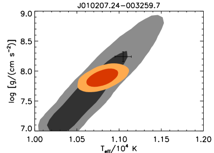
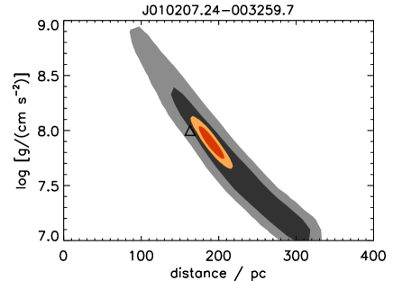
The results for most of the 34 candidate halo WDs are explained by the general arguments given above, but it is useful to investigate a few of sources in greater detail.

Of particular interest are the three objects for which spectroscopic surface gravity estimates given by Eisenstein et al. (2006) are significantly higher than the fiducial value of $\log{\mbox{\em{g}}}\simeq 7.9$: SDSS J005906.78$+$001725.2, with ${\log\hat{g}}=8.53\pm 0.38$; SDSS J010225.13$-$005458.4, with ${\log\hat{g}}=8.95\pm 0.06$; and SDSS J014247.10$+$005228.4, with ${\log\hat{g}}=8.82\pm 0.11$. The first of these was identified as a DZ type WD by Kleinman et al. (2004), and it is perhaps not surprising that the DA and DB atmosphere fits presented here and in V07 do not match the spectroscopic estimate. The latter two objects were identified as DA type WDs by Eisenstein et al. (2006). There are no UKIDSS measurements for these two stars, and the goodness–of–fit to the SDSS photometry shows nothing unusual. The implication is that these objects have intrinsically unusual surface gravity, and that the photometry is insufficient to add any information to the expectations of the $\log{\mbox{\em{g}}}$ prior. It further follows that, because of the direction of the degeneracy between $g$ and $D$, a higher value of $\log{\mbox{\em{g}}}$ would imply a significantly lower distance, and hence, lower $V_{\mathrm{tan}}$.

There are also three WDs seen in Fig. 10 (b) with strikingly high Bayesian estimates for $V_{\mathrm{tan}}$ compared with the V07 estimates: SDSS J010207.24$-$003259.7, with ${\hat{V}_{\mathrm{tan}}}\simeq 334{\mbox{\rm\,\,km}}{\mbox{\rm\,\,s}}^{-1}$, SDSS J024837.53$-$003123.9, with ${\hat{V}_{\mathrm{tan}}}\simeq 328{\mbox{\rm\,\,km}}{\mbox{\rm\,\,s}}^{-1}$, and SDSS J223808.18$+$003247.9, with ${\hat{V}_{\mathrm{tan}}}\simeq 289{\mbox{\rm\,\,km}}{\mbox{\rm\,\,s}}^{-1}$. There are UKIDSS observations for all three stars and, fortuitously, spectroscopic $\log{\mbox{\em{g}}}$ estimates given by Eisenstein et al. (2006) for the first two, the marginalised posterior distributions for which are shown in Figs. 13 and 14, respectively. For SDSS J010207.24$-$003259.7 the spectroscopic estimate of ${\log\hat{g}}=8.24\pm 0.08$ implies that it is probably not a viable halo candidate. The spectroscopic $\log{\mbox{\em{g}}}$ estimates for SDSS J024837.53$-$003123.9 are consistent with the Bayesian estimates, and hence imply this WD may have genuinely unusual dynamics. The fit for the third object, SDSS J223808.18$+$003247.9, which does not have spectroscopic data, is disastrously bad for both H and He models, with or without UKIDSS data.

SDSS J024837.53$-$003123.9 has duplicate observations in the Eisenstein et al. (2006) sample (see the left panel of Fig. 14), and it is interesting to note that the error bars given for $T_{\mathrm{eff}}$ for these repeated observations are marginally inconsistent with each other at face value (as well as being systematically higher than the Bayesian estimate, as mentioned above). The temperature uncertainties from the photometry are comparably precise to those from spectroscopy, although the surface gravity is only constrained by the spectroscopic data.

Figure 14: Same as Fig. 13(a), but for the candidate halo WD SDSS J024837.53$-$003123.9. The two points with errors are the Eisenstein et al. (2006) fits to the two SDSS spectra of this WD.

Although the model constraints on SDSS J030433.61$-$002733.2 are not interesting in themselves it is important to note that the UKIDSS data associated with this object in V07 is results from an incorrect cross-match to a much cooler star $3\aas@@fstack{\prime\prime}5$ away.

6.2 Candidate ultra-cool white dwarfs

Table 5: Estimated H atmosphere model parameters of the 24 V07 candidate ultra-cool WDs, obtained using the informative prior defined in Eq. (9).

object	$T_{\mathrm{eff}}$	$\log{\mbox{\em{g}}}$	$M$	$T$	$D$	$V_{\mathrm{tan}}$
	(K)		$(M_{\odot})$	(yr)	(pc)	(km s-1)
SDSS J001107.57$-$003102.8	$(3.64\pm 0.04)\times 10^{3}$	$7.36\pm 0.06$	$0.27\pm 0.02$	$(4.28\pm 0.37)\times 10^{9}$	$105\pm 3$	$28\pm 3$
SDSS J004843.28$-$003820.0	$(3.72\pm 0.05)\times 10^{3}$	$7.53\pm 0.09$	$0.34\pm 0.04$	$(5.07\pm 0.57)\times 10^{9}$	$146\pm 6$	$37\pm 6$
SDSS J012102.99$-$003833.6	$(3.93\pm 0.04)\times 10^{3}$	$7.75\pm 0.07$	$0.45\pm 0.03$	$(6.24\pm 0.66)\times 10^{9}$	$67\pm 3$	$39\pm 2$
SDSS J013302.17$+$010201.3	$(3.62\pm 0.10)\times 10^{3}$	$7.62\pm 0.10$	$0.38\pm 0.05$	$(6.13\pm 0.75)\times 10^{9}$	$145\pm 7$	$34\pm 6$
SDSS J030144.09$-$004439.5	$(3.62\pm 0.05)\times 10^{3}$	$7.77\pm 0.05$	$0.46\pm 0.03$	$(7.28\pm 0.52)\times 10^{9}$	$50\pm 2$	$132\pm 4$
SDSS J204332.97$+$011436.2	$(3.56\pm 0.07)\times 10^{3}$	$7.62\pm 0.09$	$0.38\pm 0.05$	$(6.35\pm 0.73)\times 10^{9}$	$139\pm 7$	$38\pm 9$
SDSS J205010.17$+$003233.7	$(3.85\pm 0.14)\times 10^{3}$	$7.85\pm 0.10$	$0.50\pm 0.05$	$(7.55\pm 1.14)\times 10^{9}$	$92\pm 7$	$24\pm 6$
SDSS J205132.05$+$000353.6	$(3.46\pm 0.04)\times 10^{3}$	$7.05\pm 0.04$	$0.17\pm 0.01$	$(3.18\pm 0.17)\times 10^{9}$	$69\pm 2$	$331\pm 9$
SDSS J210742.26$-$002354.1	$(3.49\pm 0.08)\times 10^{3}$	$7.77\pm 0.09$	$0.46\pm 0.05$	$(7.86\pm 0.81)\times 10^{9}$	$109\pm 5$	$42\pm 6$
SDSS J212216.01$-$010715.2	$(4.09\pm 0.06)\times 10^{3}$	$7.91\pm 0.10$	$0.53\pm 0.05$	$(7.53\pm 1.23)\times 10^{9}$	$105\pm 7$	$84\pm 7$
SDSS J212930.25$-$003411.5	$(3.93\pm 0.06)\times 10^{3}$	$7.98\pm 0.10$	$0.57\pm 0.06$	$(8.56\pm 0.98)\times 10^{9}$	$76\pm 6$	$154\pm 11$
SDSS J214108.42$+$002629.5	$(3.60\pm 0.10)\times 10^{3}$	$7.60\pm 0.10$	$0.37\pm 0.05$	$(6.03\pm 0.73)\times 10^{9}$	$150\pm 8$	$38\pm 8$
SDSS J220455.03$-$001750.6	$(3.76\pm 0.14)\times 10^{3}$	$7.97\pm 0.10$	$0.57\pm 0.06$	$(8.97\pm 1.06)\times 10^{9}$	$81\pm 7$	$41\pm 4$
SDSS J223105.29$+$004941.9	$(3.72\pm 0.04)\times 10^{3}$	$7.49\pm 0.07$	$0.32\pm 0.03$	$(4.78\pm 0.41)\times 10^{9}$	$113\pm 3$	$61\pm 3$
SDSS J223520.19$-$003623.6	$(3.74\pm 0.10)\times 10^{3}$	$7.91\pm 0.09$	$0.53\pm 0.05$	$(8.41\pm 1.17)\times 10^{9}$	$110\pm 7$	$73\pm 6$
SDSS J223715.32$-$002939.2	$(3.30\pm 0.06)\times 10^{3}$	$7.72\pm 0.08$	$0.43\pm 0.04$	$(8.05\pm 0.60)\times 10^{9}$	$99\pm 4$	$30\pm 3$
SDSS J223954.07$+$001849.2	$(4.22\pm 0.06)\times 10^{3}$	$7.79\pm 0.09$	$0.47\pm 0.05$	$(6.00\pm 0.91)\times 10^{9}$	$79\pm 4$	$41\pm 3$
SDSS J224206.19$+$004822.7	$(3.40\pm 0.03)\times 10^{3}$	$8.29\pm 0.06$	$0.77\pm 0.04$	$(1.07\pm 0.01)\times 10^{10}$	$24\pm 1$	$18\pm 1$
SDSS J224845.93$-$005407.0	$(4.02\pm 0.05)\times 10^{3}$	$7.93\pm 0.10$	$0.54\pm 0.06$	$(7.90\pm 1.22)\times 10^{9}$	$91\pm 6$	$88\pm 7$
SDSS J225244.51$+$000918.6	$(3.73\pm 0.14)\times 10^{3}$	$7.94\pm 0.10$	$0.55\pm 0.06$	$(8.70\pm 1.25)\times 10^{9}$	$96\pm 9$	$39\pm 5$
SDSS J232115.67$+$010223.8	$(4.46\pm 0.03)\times 10^{3}$	$7.94\pm 0.10$	$0.55\pm 0.06$	$(6.79\pm 1.07)\times 10^{9}$	$53\pm 3$	$68\pm 5$
SDSS J233055.19$+$002852.2	$(4.23\pm 0.03)\times 10^{3}$	$7.89\pm 0.08$	$0.52\pm 0.04$	$(7.08\pm 0.96)\times 10^{9}$	$49\pm 2$	$39\pm 2$
SDSS J233818.56$-$004146.2	$(3.70\pm 0.06)\times 10^{3}$	$7.72\pm 0.09$	$0.43\pm 0.04$	$(6.66\pm 0.82)\times 10^{9}$	$122\pm 6$	$82\pm 6$
SDSS J234646.06$-$003527.6	$(3.70\pm 0.06)\times 10^{3}$	$7.55\pm 0.09$	$0.35\pm 0.04$	$(5.24\pm 0.60)\times 10^{9}$	$143\pm 6$	$30\pm 5$

Table 6: Estimated He atmosphere model parameters of the 24 V07 candidate ultra-cool WDs, obtained using the informative prior defined in Eq. (9).

object	$T_{\mathrm{eff}}$	$\log{\mbox{\em{g}}}$	$M$	$T$	$D$	$V_{\mathrm{tan}}$
	(K)		$(M_{\odot})$	(yr)	(pc)	(km s-1)
SDSS J001107.57$-$003102.8	$(4.49\pm 0.04)\times 10^{3}$	$7.99\pm 0.11$	$0.57\pm 0.06$	$(6.68\pm 0.78)\times 10^{9}$	$106\pm 9$	$29\pm 4$
SDSS J004843.28$-$003820.0	$(4.42\pm 0.04)\times 10^{3}$	$7.93\pm 0.10$	$0.53\pm 0.05$	$(6.41\pm 1.00)\times 10^{9}$	$154\pm 11$	$39\pm 7$
SDSS J012102.99$-$003833.6	$(4.65\pm 0.02)\times 10^{3}$	$7.92\pm 0.10$	$0.53\pm 0.05$	$(5.83\pm 1.00)\times 10^{9}$	$83\pm 5$	$48\pm 4$
SDSS J013302.17$+$010201.3	$(4.35\pm 0.05)\times 10^{3}$	$7.91\pm 0.10$	$0.53\pm 0.05$	$(6.42\pm 1.07)\times 10^{9}$	$159\pm 12$	$38\pm 7$
SDSS J030144.09$-$004439.5	$(4.60\pm 0.02)\times 10^{3}$	$7.90\pm 0.10$	$0.52\pm 0.05$	$(5.74\pm 1.05)\times 10^{9}$	$70\pm 4$	$185\pm 12$
SDSS J204332.97$+$011436.2	$(4.33\pm 0.05)\times 10^{3}$	$7.90\pm 0.10$	$0.52\pm 0.05$	$(6.39\pm 1.09)\times 10^{9}$	$155\pm 12$	$43\pm 10$
SDSS J205010.17$+$003233.7	$(4.60\pm 0.06)\times 10^{3}$	$7.90\pm 0.10$	$0.52\pm 0.05$	$(5.75\pm 1.05)\times 10^{9}$	$120\pm 9$	$31\pm 7$
SDSS J205132.05$+$000353.6	$(4.15\pm 0.04)\times 10^{3}$	$7.92\pm 0.10$	$0.53\pm 0.05$	$(6.88\pm 1.10)\times 10^{9}$	$54\pm 4$	$262\pm 21$
SDSS J210742.26$-$002354.1	$(4.52\pm 0.03)\times 10^{3}$	$7.89\pm 0.10$	$0.51\pm 0.05$	$(5.85\pm 1.06)\times 10^{9}$	$154\pm 11$	$60\pm 8$
SDSS J212216.01$-$010715.2	$(4.73\pm 0.03)\times 10^{3}$	$7.89\pm 0.10$	$0.51\pm 0.05$	$(5.44\pm 1.00)\times 10^{9}$	$142\pm 9$	$115\pm 9$
SDSS J212930.25$-$003411.5	$(4.71\pm 0.03)\times 10^{3}$	$7.91\pm 0.10$	$0.53\pm 0.05$	$(5.66\pm 1.01)\times 10^{9}$	$110\pm 7$	$224\pm 15$
SDSS J214108.42$+$002629.5	$(4.32\pm 0.05)\times 10^{3}$	$7.91\pm 0.10$	$0.53\pm 0.05$	$(6.46\pm 1.09)\times 10^{9}$	$162\pm 12$	$41\pm 9$
SDSS J220455.03$-$001750.6	$(4.66\pm 0.03)\times 10^{3}$	$7.89\pm 0.10$	$0.51\pm 0.05$	$(5.54\pm 1.01)\times 10^{9}$	$124\pm 8$	$63\pm 5$
SDSS J223105.29$+$004941.9	$(4.55\pm 0.03)\times 10^{3}$	$7.96\pm 0.10$	$0.55\pm 0.06$	$(6.35\pm 0.89)\times 10^{9}$	$123\pm 9$	$67\pm 6$
SDSS J223520.19$-$003623.6	$(4.64\pm 0.03)\times 10^{3}$	$7.90\pm 0.10$	$0.52\pm 0.05$	$(5.69\pm 1.05)\times 10^{9}$	$160\pm 11$	$106\pm 8$
SDSS J223715.32$-$002939.2	$(4.54\pm 0.03)\times 10^{3}$	$7.86\pm 0.10$	$0.50\pm 0.05$	$(5.61\pm 1.00)\times 10^{9}$	$149\pm 10$	$46\pm 6$
SDSS J223954.07$+$001849.2	$(4.60\pm 0.04)\times 10^{3}$	$7.90\pm 0.09$	$0.52\pm 0.05$	$(5.75\pm 1.02)\times 10^{9}$	$89\pm 6$	$46\pm 3$
SDSS J224206.19$+$004822.7	$(4.84\pm 0.02)\times 10^{3}$	$7.66\pm 0.09$	$0.40\pm 0.05$	$(3.48\pm 0.63)\times 10^{9}$	$65\pm 4$	$50\pm 3$
SDSS J224845.93$-$005407.0	$(4.72\pm 0.03)\times 10^{3}$	$7.93\pm 0.10$	$0.53\pm 0.05$	$(5.77\pm 0.96)\times 10^{9}$	$125\pm 9$	$121\pm 9$
SDSS J225244.51$+$000918.6	$(4.65\pm 0.03)\times 10^{3}$	$7.89\pm 0.10$	$0.52\pm 0.05$	$(5.60\pm 1.04)\times 10^{9}$	$145\pm 10$	$59\pm 7$
SDSS J232115.67$+$010223.8	$(4.87\pm 0.02)\times 10^{3}$	$7.92\pm 0.09$	$0.53\pm 0.05$	$(5.40\pm 0.92)\times 10^{9}$	$65\pm 4$	$84\pm 5$
SDSS J233055.19$+$002852.2	$(4.76\pm 0.02)\times 10^{3}$	$7.91\pm 0.10$	$0.52\pm 0.05$	$(5.54\pm 1.01)\times 10^{9}$	$62\pm 4$	$49\pm 3$
SDSS J233818.56$-$004146.2	$(4.55\pm 0.03)\times 10^{3}$	$7.93\pm 0.10$	$0.54\pm 0.05$	$(6.14\pm 1.01)\times 10^{9}$	$153\pm 11$	$103\pm 9$
SDSS J234646.06$-$003527.6	$(4.42\pm 0.04)\times 10^{3}$	$7.93\pm 0.10$	$0.54\pm 0.05$	$(6.42\pm 0.99)\times 10^{9}$	$154\pm 11$	$32\pm 6$

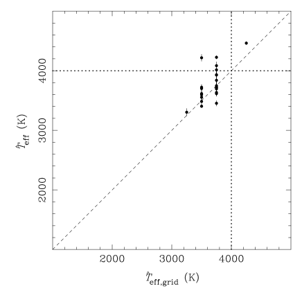
The 24 candidate ultra-cool WDs identified by V07 were analysed using the techniques described in Section 2 and Section 3, giving parameter estimates and evidence values for both H and He atmosphere models. The results obtained using the informative prior defined in Section 4 are presented in Tables 5 and 6. The Bayesian parameter fits are compared to those obtained by V07 in Fig. 15 for the informative prior.

For the ultra-cool WDs, the temperature comparison shown in Fig. 15 is the critical test as it was on the basis of $\hat{T}_{\mathrm{eff,grid}}$ that these 24 objects were selected. The discretisation on the horizontal axis is again due to the grid-based fitting of V07. The slight tendency for the Bayesian fits to have a higher $\hat{T}_{\mathrm{eff}}$ is due to the selection effect that resulted in the more pronounced distance bias discussed in Section 6.1.

Figure 15: The estimated effective temperature, $\hat{T}_{\mathrm{eff}}$, of the 24 candidate ultra-cool WDs as found by V07 and obtained using the Bayesian method described here (for H atmosphere models, with the Galactic model priors). The selection criterion as an ultra-cool WD, $\hat{T}_{\mathrm{eff}}\leq 4000{\mbox{\rm\,\,K}}$, adopted by V07 is shown as the vertical and horizontal dotted lines. One source, SDSS J232115.67$+$010223.8, is listed in this sample despite an estimated effective temperature above this nominal limit.

The various distance estimates for the ultra-cool WDs are also in broad agreement. Comparing the results obtained using the non-informative prior with those provided by V07 reveals only a small scatter due to the best-fit models lying between the model grid points. The Bayesian distance estimates obtained from the informative prior and those given by V07 also exhibit systematic differences, with the former tending towards the average value of $\hat{D}\simeq 100{\mbox{\rm\,\,pc}}$.

Given that the Bayesian distance estimates are in agreement with those of V07, it is not surprising that the same holds for the tangential velocity estimates. The only significant exception to this is SDSS J205132.05$+$000353.6, for which the H fit shown is probably inappropriate, confirming the findings of V07 that this WD has a He atmosphere. This object is discussed further in Section 6.2.1.

Table 7: Model selection quantities for the 24 V07 candidate ultra-cool WDs, where columns 2 and 3 are the best fit $\log{\mbox{\em{g}}}$ values estimated using the uninformative $g$ prior. UKIDSS data have been used where available. The final column states whether the model selection probability of ${\mathrm{H}}$ versus ${\mathrm{He}}$ is driven by the data, the informative $g$ prior, or the 10:1 model prior.

object	$\log g_{\mathrm{H}}$	$\log g_{\mathrm{He}}$	$\chi^{2}_{\rm min,{\mathrm{H}}}$	$\chi^{2}_{\rm min,{\mathrm{He}}}$	$E_{\mathrm{H}}$	$E_{\mathrm{He}}$	$P_{\mathrm{H}}$	notes
SDSS J001107.57$-$003102.8	7.05	8.91	16.3	12.0	$2.0\times 10^{-16}$	$4.4\times 10^{-10}$	$4.2\times 10^{-06}$	data
SDSS J004843.28$-$003820.0	7.05	8.80	44.3	22.7	$3.6\times 10^{-18}$	$2.7\times 10^{-07}$	$1.2\times 10^{-10}$	data, neither model good fit
SDSS J012102.99$-$003833.6	7.59	8.21	29.8	4.7	$4.1\times 10^{-11}$	$2.6\times 10^{-05}$	$1.4\times 10^{-05}$	data
SDSS J013302.17$+$010201.3	7.07	8.62	34.6	21.6	$5.2\times 10^{-13}$	$4.9\times 10^{-05}$	$9.5\times 10^{-08}$	data, neither model good fit
SDSS J030144.09$-$004439.5	7.72	7.90	12.7	16.3	$2.6\times 10^{-06}$	$1.2\times 10^{-06}$	$0.95$	data and model prior
SDSS J204332.97$+$011436.2	7.07	8.46	31.6	15.8	$2.2\times 10^{-12}$	$3.3\times 10^{-03}$	$6.1\times 10^{-09}$	data and $g$ prior
SDSS J205010.17$+$003233.7	7.38	8.20	3.8	7.0	$1.8\times 10^{+02}$	$2.4\times 10^{+01}$	$0.99$	data and model prior
SDSS J205132.05$+$000353.6	7.01	8.85	272.6	22.5	$0.0$	$8.8\times 10^{-09}$	$0.00$	data, neither model good fit
SDSS J210742.26$-$002354.1	7.45	7.75	7.1	0.9	$1.9\times 10^{-02}$	$5.4$	$3.1\times 10^{-02}$	data and $g$ prior
SDSS J212216.01$-$010715.2	8.46	7.91	9.2	1.6	$2.5\times 10^{-03}$	$1.3$	$1.8\times 10^{-02}$	data and $g$ prior
SDSS J212930.25$-$003411.5	8.31	8.45	5.7	0.2	$7.8\times 10^{-04}$	$4.0\times 10^{-02}$	$0.15$	data
SDSS J214108.42$+$002629.5	7.06	8.68	35.5	20.1	$8.8\times 10^{-14}$	$7.9\times 10^{-05}$	$1.0\times 10^{-08}$	data, neither model good fit
SDSS J220455.03$-$001750.6	8.15	7.83	23.5	7.4	$1.3\times 10^{-06}$	$2.5\times 10^{-02}$	$4.7\times 10^{-04}$	data
SDSS J223105.29$+$004941.9	7.07	8.84	10.2	4.0	$2.3\times 10^{-12}$	$1.7\times 10^{-06}$	$1.2\times 10^{-05}$	data
SDSS J223520.19$-$003623.6	7.87	8.15	7.5	1.7	$8.9\times 10^{-02}$	$6.8\times 10^{-01}$	$0.54$	model prior and $g$ prior
SDSS J223715.32$-$002939.2	7.23	7.44	19.6	15.3	$5.2\times 10^{-07}$	$7.0\times 10^{-04}$	$6.7\times 10^{-03}$	data and $g$ prior
SDSS J223954.07$+$001849.2	7.28	8.01	34.8	19.6	$1.3\times 10^{-10}$	$5.3\times 10^{-06}$	$2.1\times 10^{-04}$	data and $g$ prior
SDSS J224206.19$+$004822.7	8.58	7.07	44.8	286.1	$5.0\times 10^{-21}$	$0.0$	$1.00$	data, neither model good fit
SDSS J224845.93$-$005407.0	8.09	8.48	14.7	8.9	$4.4\times 10^{-05}$	$4.4\times 10^{-05}$	$0.90$	model prior and $g$ prior
SDSS J225244.51$+$000918.6	8.07	7.96	8.3	1.9	$2.9\times 10^{-02}$	$1.3$	$0.17$	data and $g$ prior
SDSS J232115.67$+$010223.8	8.46	8.43	19.1	4.8	$6.2\times 10^{-08}$	$9.2\times 10^{-05}$	$6.1\times 10^{-03}$	data
SDSS J233055.19$+$002852.2	7.89	8.08	30.4	6.0	$1.7\times 10^{-10}$	$1.6\times 10^{-05}$	$9.3\times 10^{-05}$	data
SDSS J233818.56$-$004146.2	7.21	8.76	11.2	13.3	$3.0\times 10^{-05}$	$1.5\times 10^{-05}$	$0.95$	model prior and $g$ prior
SDSS J234646.06$-$003527.6	7.06	8.82	30.7	22.8	$1.4\times 10^{-14}$	$9.8\times 10^{-08}$	$1.3\times 10^{-06}$	data, neither model good fit

The model comparison results for the ultra-cool sample are summarised in Table 7. The most striking result is that 18 out of the 24 candidate ultra-cool WDs have a high probability of being He stars, despite the strong model prior that H stars should be $\sim 10$ times more common. The same conclusion is also implied by the optical data alone, although it is perhaps more revealing that several stars are poor fits to both the H and He models. It is also interesting to note that the best-fit temperatures of the He stars are typically higher than for H in this region of parameter space. Thus it is possible that selecting WDs on the basis of having a low $\hat{T}_{\mathrm{eff}}$ from H fits results in also selecting He stars with less extreme temperatures.

6.2.1 Notes on individual objects

Three stars in the sample of candidate ultra-cool WDs have been spectroscopically confirmed as being of type DC. SDSS J224206$+$004822 and SDSS J233055$+$002852 were initially discovered by Kilic et al. (2006) who, from photometric fits with $\log{\mbox{\em{g}}}=8.0$, found $\hat{T}_{\mathrm{eff}}=3400{\mbox{\rm\,\,K}}$ and $\hat{T}_{\mathrm{eff}}=4100{\mbox{\rm\,\,K}}$, respectively. Applying the Bayesian approach described in Section 2.2 and using the informative $\log{\mbox{\em{g}}}$ prior given in Section 4 gives $\hat{T}_{\mathrm{eff}}=3400\pm 30{\mbox{\rm\,\,K}}$ for SDSS J224206$+$004822 (where H is a better fit but neither model fits the data well), and $\hat{T}_{\mathrm{eff}}=4760\pm 20{\mbox{\rm\,\,K}}$ for SDSS J233055$+$002852 (where He is clearly a better fit). SDSS J232115.67$+$010223.8 was reported by Carollo et al. (2006) as being of type DC; the Bayesian results imply that this star most probably has a He atmosphere, with $\hat{T}_{\mathrm{eff}}=4870\pm 20{\mbox{\rm\,\,K}}$.

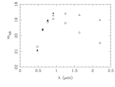
Only one of the 24 ultra-cool WD candidates identified by V07 was found to definitely have a He-dominated atmosphere. Given the strong degeneracies in the photometric WD fitting, it was possible that this conclusion came about only due to the sparse grid of H models ‘straddling’ the good fit locus while one of the He models fortuitously landed on it. Nonetheless, these inferences are supported by the more thorough MCMC exploration of the model space, although the fact that neither atmospheric species results in a good fit (as shown in Fig. 16) leaves the possibility that SDSS J205132$+$000353 is not a WD at all. This possibility has been corroborated by Kilic (private communication), who did not detect an appreciable proper motion from multi-epoch astrometry of this source, implying it is more likely to be a quasar, or other extra-Galactic object. These observations are at odds with proper motion of $\hat{\mu}=(1.02\pm 0.01){\mbox{\rm\,\,arcsec}}{\mbox{\rm\,\,yr}}^{-1}$ quoted by V07; however there are two other stars within a few arcsec of SDSS J205132$+$000353, and so it is possible that the automated matching algorithm of Bramich et al. (2008) was unable to process this complicated case.

SDSS J205132$+$000353 and SDSS J212930.25$-$003411.5 have very high ${\hat{V}_{\mathrm{tan}}}$ values of $262\pm 21{\mbox{\rm\,\,km}}{\mbox{\rm\,\,s}}^{-1}$ and $224\pm 15{\mbox{\rm\,\,km}}{\mbox{\rm\,\,s}}^{-1}$, respectively. The fact that the former is not a good fit to either model atmosphere probably invalidates the estimate of $V_{\mathrm{tan}}$, but the latter remains a good halo candidate.

Figure 16: Photometry in the $g$, $r$, $i$ and $z$bands (solid dots) of the probable He WD SDSS J205132$+$000353, compared to the best-fit H models (open squares) and He models (open triangles) in the $u$, $g$, $r$, $i$, $z$, $J$, $H$ and $K$ bands. The photometric errors are $\sim 0.02$, and smaller than the symbol size.

7 Conclusions

WDs can be identified reliably using just photometric and astrometric information, but the utility of large samples generated in this way is limited if WDs cannot also be characterised without recourse to spectroscopy. The degree to which this is possible has been assessed here by using Bayesian methods to include vital prior information in the parameter estimation process. For most WDs observed with SDSS precision photometry (or per cent-level photometry, but only in bands redder than $u$) only their effective temperature and solid angle can be constrained unambigously. However this very generic degeneracy can be broken by utilising the prior information (from spectroscopic modelling) that most WDs have surface gravities of $7.7\la\log{\mbox{\em{g}}}\la 8.1$.

The power of this approach was demonstrated by applying it to the samples of candidate halo and ultra-cool WDs generated by V07 from multi-epoch SDSS Stripe 82 data. This confirms their identification of ultra-cool stars (as the photometric data constrain the temperature well) but implies that most of the candidate halo stars are members of the more numerous thick disk population with unusual observed colours caused by photometric noise. This is a particular case of a very general result, that it is almost impossible to reliably identify a small number of outliers if there are sufficiently many members of the more dominant population to scatter to the parameter space of interest.

The one situation in which photometric data are likely to give definitive WD parameter estimates without prior information is if per cent-level photometry is available in the $u$, $g$ and $r$ (or similar) bands for H atmosphere WDs with $10000{\mbox{\rm\,\,K}}\la T_{\mathrm{eff}}\la 18000{\mbox{\rm\,\,K}}$. As shown by Ivezić et al. (2007), the loci of observed colours of WDs in SDSS Stripe 82 exhibit an obvious separation between H and He models (see Fig. 1), and the next stage of this work will be to analyse a sample of such sources. This should also have the additional benefit of giving a more accurate surface gravity prior than used here (in which the numbers of WDs with non-fiducial surface gravities are almost certainly under-estimated). Another important extension to this work will be to add a velocity prior from Galactic dynamics: for most WDs this will not be important, but it will be critical to obtaining the most stringent constraints on potential halo objects. An added side-benefit of being able to identify halo objects dynamically will be to place empirical constraints on the temperature and age distribution of halo WDs (cf. Hansen 2001; Pauli et al. 2006). Further, while the effect of the ISM has not been included in this work (in part to follow the assumptions of the V07 analysis), it would be straightforward to include a full ISM model or Galactic extinction template as described in Section 2.

These results have particularly relevance to up-coming large-scale deep optical surveys such as the SkyMapper survey (Keller et al., 2007), the Dark Energy Survey (DES; Flaugher et al. 2006), the Panoramic Survey Telescope And Rapid Response System (Pan–STARRS; Kaiser et al. 2002) and the Large Synoptic Survey Telescope (LSST; Ivezić et al. 2008). In the context of WD studies, a critical distinction between these projects is that only SkyMapper and LSST plan to observe in the $u$ band. With LSST expected to reach $\mbox{$u$}\simeq 26$ over half the sky, it should yield a sample of $\sim 10^{6}$ WDs with sufficiently precise photometric and astrometric measurements to give accurate distances and tangential velocities. Combined with the methods presented here, these data will provide an unprecedented understanding of the Galaxy’s WD population.

References

- Alcock et al. (2000) Alcock C., et al., 2000, ApJ, 542, 281
- Beauchamp et al. (1996) Beauchamp A., Wesemael F., Bergeron P., Liebert J., Saffer R. A., 1996, in Jeffery C. S., Heber U., eds, Hydrogen Deficient Stars Vol. 96 of Astronomical Society of the Pacific Conference Series. p. 295
- Bergeron & Leggett (2002) Bergeron P., Leggett S. K., 2002, ApJ, 580, 1070
- Bergeron et al. (2001) Bergeron P., Leggett S. K., Ruiz M. T., 2001, ApJS, 133, 413
- Bergeron et al. (1997) Bergeron P., Ruiz M. T., Leggett S. K., 1997, ApJS, 108, 339
- Bergeron et al. (1992) Bergeron P., Saffer R. A., Liebert J., 1992, ApJ, 394, 228
- Bergeron et al. (1995) Bergeron P., Wesemael F., Beauchamp A., 1995, PASP, 107, 1047
- Bergeron et al. (1990) Bergeron P., Wesemael F., Fontaine G., Liebert J., 1990, ApJL, 351, L21
- Bramich et al. (2008) Bramich D. M., et al., 2008, MNRAS, 386, 887
- Carollo et al. (2006) Carollo D., Bucciarelli B., Hodgkin S. T., Lattanzi M. G., McLean B., Morbidelli R., Smart R. L., Spagna A., Terranegra L., 2006, A&A, 448, 579
- Chabrier (1999) Chabrier G., 1999, ApJL, 513, L103
- Eisenstein et al. (2006) Eisenstein D. J., et al., 2006, ApJS, 167, 40
- Engelbrecht & Koester (2007) Engelbrecht A., Koester D., 2007, in Napiwotzki R., Burleigh M. R., eds, 15th European Workshop on White Dwarfs Vol. 372 of Astronomical Society of the Pacific Conference Series. p. 289
- Finley et al. (1997) Finley D. S., Koester D., Basri G., 1997, ApJ, 488, 375
- Flaugher et al. (2006) Flaugher B., et al., 2006, in BAAS Vol. 38 of BAAS. p. 928
- Fontaine et al. (2005) Fontaine G., Bergeron P., Brassard P., 2005, in Sion E. M., Vennes S., Shipman H. L., eds, White dwarfs: cosmological and galactic probes Vol. 332 of Astrophysics and Space Science Library, Old ultracool white dwarfs as cosmological probes. pp 3–13
- Fontaine et al. (2001) Fontaine G., Brassard P., Bergeron P., 2001, PASP, 113, 409
- Gates et al. (2004) Gates E., et al., 2004, ApJL, 612, L129
- Gelman, A. and Rubin, D. B. (1992) Gelman, A. and Rubin, D. B. 1992, Statistical Science, 7, 457
- Gilks et al. (1999) Gilks W. R., Richardson S., Spiegelhalter D. J., 1999, Markov Chain Monte Carlo In Practice. Chapman and Hall/CRC, Boca Raton
- Hansen (2001) Hansen B. M. S., 2001, ApJL, 558, L39
- Harris et al. (1999) Harris H. C., Dahn C. C., Vrba F. J., Henden A. A., Liebert J., Schmidt G. D., Reid I. N., 1999, ApJ, 524, 1000
- Harris et al. (2003) Harris H. C., et al., 2003, AJ, 126, 1023
- Harris et al. (2006) Harris H. C., et al., 2006, AJ, 131, 571
- Harris et al. (2008) Harris H. C., et al., 2008, ApJ, 679, 697
- Hastings (1970) Hastings W. K., 1970, Biometrika, 57, 97
- Hodgkin et al. (2000) Hodgkin S. T., Oppenheimer B. R., Hambly N. C., Jameson R. F., Smartt S. J., Steele I. A., 2000, Nature, 403, 57
- Hogg et al. (2005) Hogg D. W., Blanton M. R., Roweis S. T., Johnston K. V., 2005, ApJ, 629, 268
- Holberg & Bergeron (2006) Holberg J. B., Bergeron P., 2006, AJ, 132, 1221
- Holberg et al. (2008) Holberg J. B., Sion E. M., Oswalt T., McCook G. P., Foran S., Subasavage J. P., 2008, AJ, 135, 1225
- Ibata et al. (2000) Ibata R., Irwin M., Bienaymé O., Scholz R., Guibert J., 2000, ApJL, 532, L41
- Ivezić et al. (2007) Ivezić Ž., et al., 2007, AJ, 134, 973
- Ivezić et al. (2008) Ivezić Ž., et al., 2008, ArXiv:0805.2366
- Jaynes (2003) Jaynes E. T., 2003, Probability Theory. Cambridge University Press, Cambridge, UK
- Jordan (2007) Jordan S., 2007, in Napiwotzki R., Burleigh M. R., eds, 15th European Workshop on White Dwarfs Vol. 372 of Astronomical Society of the Pacific Conference Series. p. 139
- Jurić et al. (2008) Jurić M., et al., 2008, ApJ, 673, 864
- Kaiser et al. (2002) Kaiser N., et al., 2002, in Tyson J. A., Wolff S., eds, Society of Photo-Optical Instrumentation Engineers (SPIE) Conference Series Vol. 4836 of Society of Photo-Optical Instrumentation Engineers (SPIE) Conference Series. p. 154
- Keller et al. (2007) Keller S. C., et al., 2007, PASA, 24, 1
- Kilic et al. (2006) Kilic M., et al., 2006, AJ, 131, 582
- Kleinman et al. (2004) Kleinman S. J., et al., 2004, ApJ, 607, 426
- Lawrence et al. (2007) Lawrence A., et al., 2007, Mon. Not. Roy. Astron. Soc., 379, 1599
- Leggett et al. (1998) Leggett S. K., Ruiz M. T., Bergeron P., 1998, ApJ, 497, 294
- Liebert et al. (2005) Liebert J., Bergeron P., Holberg J. B., 2005, ApJS, 156, 47
- Maíz-Apellániz (2001) Maíz-Apellániz J., 2001, AJ, 121, 2737
- McCook & Sion (1999) McCook G. P., Sion E. M., 1999, ApJS, 121, 1
- Mestel (1952) Mestel L., 1952, MNRAS, 112, 583
- Metropolis et al. (1953) Metropolis N., Rosenbluth A. W., Rosenbluth M. N., Teller A. H., Teller E., 1953, The Journal of Chemical Physics, 21, 1087
- Neal (1993) Neal R. M., 1993, Probabilistic Inference Using Markov Chain Monte Carlo Methods, http://www.cs.toronto.edu/radford/ftp/review.pdf
- Oppenheimer et al. (2001b) Oppenheimer B. R., et al., 2001, ApJ, 550, 448
- Oppenheimer et al. (2001a) Oppenheimer B. R., Hambly N. C., Digby A. P., Hodgkin S. T., Saumon D., 2001, Science, 292, 698
- Pauli et al. (2006) Pauli E.-M., Napiwotzki R., Heber U., Altmann M., Odenkirchen M., 2006, A&A, 447, 173
- Perryman et al. (2001) Perryman M. A. C., de Boer K. S., Gilmore G., Høg E., Lattanzi M. G., Lindegren L., Luri X., Mignard F., Pace O., de Zeeuw P. T., 2001, A&A, 369, 339
- Reid (2005) Reid I. N., 2005, ARA&A, 43, 247
- Salim et al. (2004) Salim S., Rich R. M., Hansen B. M., Koopmans L. V. E., Oppenheimer B. R., Blandford R. D., 2004, ApJ, 601, 1075
- Scranton et al. (2005) Scranton R., Connolly A. J., Szalay A. S., Lupton R. H., Johnston D., Budavari T., Brinkman J., Fukugita M., 2005, AJ, submitted
- Sesar et al. (2007) Sesar B., et al., 2007, AJ, 134, 2236
- Smolčić et al. (2004) Smolčić V., et al., 2004, ApJL, 615, L141
- Torres et al. (2005) Torres S., García-Berro E., Isern J., Figueras F., 2005, MNRAS, 360, 1381
- Vidrih et al. (2007) Vidrih S., et al., 2007, MNRAS, 382, 515
- Voss et al. (2007) Voss B., Koester D., Napiwotzki R., Christlieb N., Reimers D., 2007, A&A, 470, 1079
- Wood (1992) Wood M. A., 1992, ApJ, 386, 539
- York et al. (2000) York D. G., et al., 2000, AJ, 120, 1579