Thermodynamics of itinerant magnets in a classical spin fluctuation model

Abstract

Thermodynamics of itinerant magnets is studied using a classical model with one parameter characterizing the degree of itinerancy. Monte Carlo simulations for bcc and fcc lattices are compared with the mean-field approximation and with the Onsager cavity field approximation extended to itinerant systems. The qualitative features of thermodynamics are similar to the known results of the functional integral method. It is found that magnetic short-range order is weak and almost independent on the degree of itinerancy, and the mean-field approximation describes the thermodynamics reasonably well. Ambiguity of the phase space measure for classical models is emphasized. The Onsager cavity field method is extended to itinerant systems, which involves the renormalization of both the Weiss field and the on-site exchange interaction. The predictions of this approximation are in excellent agreement with Monte Carlo results.

I Introduction

The thermodynamics of magnetic materials is often described using the Heisenberg model in which the spins are attached to lattice sites. Real magnets are much more complicated, because the magnetization is due to band electrons whose degree of localization varies between different materials. This so-called itinerancy manifests itself in the fluctuation of the magnitudes of the local moments, which may be defined in a muffin tin sphere or using a projection in an appropriate basis. Thus, the degree of itinerancy may be characterized by the relative importance of longitudinal and transverse (rotational) fluctuations of the local moments. Moriya In the localized (Heisenberg) limit the longitudinal spin fluctuations (LSF) have a large energy scale and are suppressed. This limit is approached in some magnetic insulators. Metals, on the other hand, are often quite far from this limit, because the exchange splitting and the bandwidth are typically of the same order. Experimentally, itinerancy is most clearly revealed in the paramagnetic susceptibility by the deviation of the effective moment found from the Curie-Weiss constant from the true local moment, as well as by the deviations from the Curie-Weiss law.

A large amount of work has been devoted to the thermodynamics of itinerant magnets using phenomenological Ginzburg-Landau models for weak ferromagnets MD ; LT ; Moriya or the Hubbard model and the functional integral methods. MT78 ; Hubbard ; Hasegawa ; Moriya These studies have clarified the role of LSF in thermodynamics and explained the observed behavior of the paramagnetic susceptibility. However, these methods are unsuitable for quantitative studies of realistic materials. Ginzburg-Landau expansions, as is well known, correctly describe only the contribution of long-wave fluctuations and must always be rigged with a wavevector cut-off. Such models are useful in the studies of critical phenomena, but they are irrelevant to the determination of the critical temperature itself, which is determined by short-range fluctuations. LL5 An unsatisfactory signature of Ginzburg-Landau models is the absence of any information on the short-wave components of the exchange interaction in the resulting expressions for the Curie temperature.MD ; LT ; MW In our opinion, the neglect of short-wave fluctuations in these models makes their predictions for magnetic short-range order (MSRO) also unreliable. The functional integral method, on the other hand, suffers from the necessity to make severe and ambiguous approximations.HE73

Magnetic thermodynamics has also been studied using density functional theory (DFT) by treating spin fluctuations within the adiabatic approximation Gyorffy assuming that the relevant fluctuations are well represented by constrained Dederichs noncollinear ground states. The most widespread approach is the disordered local moment (DLM) approximation Oguchi ; Gyorffy which relies on the single-site approximation and is designed to approximate the DFT ground state of a system with random directions of the local moments. The LSF have been neglected in all implementations of this approach so far, restricting its application to magnets which are close to the localized limit. In particular, the DLM method neglecting LSF fails for (strongly itinerant) nickel where it finds vanishing local moment in the paramagnetic phase.Staunton

Other authors studied itinerant thermodynamics by mapping the results of first-principles energies for various spin configurations (including both transverse and longitudinal fluctuations) to a classical Hamiltonian in which variable local moments play the role of dynamical variables, and then exploring the thermodynamics of this Hamiltonian using either the variational principle in reciprocal space Uhl or Monte Carlo (MC) simulations in real space. Rosengaard ; Lezaic ; Ruban These calculations clearly show that LSF, as expected, are very important in nickel. Moreover, they revealed only weak magnetic short-range order (MSRO) above the Curie temperature $T_{c}$ for both Fe and Ni, which is similar to the Heisenberg model. These results are consistent with the fact that in any lattice model with no frustration all correlation corrections to the mean-field approximation (outside of the critical region) should be small in the parameter $1/z$, where $z$ is the number of neighbors within the interaction range. DMFT On the other hand, very strong MSRO above $T_{c}$ was found Antropov in Ni using the ab initio spin dynamics method, which, similar to DLM, is based on the adiabatic approximation and neglects LSF.

Classical models with variable local moments seem to capture the important qualitative features of the thermodynamics of itinerant magnets which are similar to the predictions of the functional integral method. However, these models have been built and studied only for a few particular materials, and a general study of their thermodynamic properties has not been undertaken. Such a study is useful as a step to more refined models with the advantage that numerically exact results for a classical model are easily accessible through Monte Carlo simulations. Therefore, in this paper we explore the thermodynamics of a classical spin fluctuation model as a function of the degree of itinerancy using MC simulations and simple analytic approximations. We emphasize that here we are not concerned with the “mapping” procedure (which can be quite challenging) but rather focus on the other separate part of the program, i.e. on the determination of thermodynamics once the Hamiltonian has been defined. We therefore restrict ourselves to the simplest possible realization of this model which includes only one free parameter characterizing the degree of itinerancy.

II Model

Our model is a lattice version of the phenomenological model of Murata and Doniach MD written with a vector order parameter Moriya :

$$H=\frac{1}{2}\sum_{\mathbf{q}}\chi^{-1}(\mathbf{q})\mathbf{m}_{\mathbf{q}}\mathbf{m}_{-\mathbf{q}}+\frac{B}{4}\sum_{i}m_{i}^{4}$$

$$=\sum_{i}\left[\frac{1}{2}\left(\chi^{-1}_{00}-I\right)m^{2}_{i}+\frac{B}{4}m_{i}^{4}\right]-\frac{1}{2}\sum_{i\neq j}J_{ij}\mathbf{m}_{i}\mathbf{m}_{j}.$$ (1)

Here $\mathbf{m}_{i}$ denotes the magnetic moment at site i whose length is unrestricted, and $I$ the Stoner exchange-correlation parameter. We have separately written the local $\chi^{-1}_{00}=\partial B_{i}/\partial m_{i}$ and nonlocal $J_{ij}=-\chi^{-1}_{ij}$ parts of the unenhanced inverse susceptibility. This model involves a number of simplifying assumptions: (1) It is classical in the sense that $\mathbf{m}_{i}$ are dynamical variables and not operators. (2) Both local and nonlocal parts of the inverse susceptibility are considered to be independent of the magnetic state and isotropic. In general, $\chi^{-1}_{ij}$ is a Cartesian tensor which depends on the magnetic state and reduces to a scalar only in the paramagnetic state. (3) Nonlinear effects are included only through a local fourth-order term, similar to the Murata-Doniach model.

Model (1) is somewhat similar to that used to represent the unified spin fluctuation theoryMT78 classically (see Ref. Moriya, , Ch. 7, and also Ref. Kubler, ), with an important difference: the energy of LSFs is included as a function of local dynamical variables $\mathbf{m}_{i}$, rather than that of one global parameter $\langle m^{2}_{i}\rangle$. This difference is similar to that between the Heisenberg model and the spherical approximation to it.

In the ground state all local moments are parallel and we recover the Stoner model which is ferromagnetic if $IN(E_{F})>1$, where $N(E_{F})=\chi(0)$ is the density of states at the Fermi level in the nonmagnetic state. This Stoner criterion can also be written as $(I+J_{0})>\chi^{-1}_{00}$ where $J_{0}=\sum_{j}J_{ij}$. On the other hand, in the paramagnetic or non-magnetic matrix, local moments exist in the Anderson sense only if $I>\chi^{-1}_{00}$ which is stricter than the Stoner criterion. We will call this the Anderson criterion. (Note that $\chi^{-1}_{00}\neq 1/\chi_{00}$.)

Introducing reduced local moments $\mathbf{x}_{i}=\mathbf{m}_{i}/m_{0}$, where $m_{0}$ is the value of all $m_{i}$ at $T=0$, the Hamiltonian (1) can be conveniently parameterized:

$$H^{\prime}\equiv\frac{H}{J_{0}m^{2}_{0}}=\sum_{i}E(x_{i})-\frac{1}{2}\sum_{i\neq j}\frac{J_{ij}}{J_{0}}\mathbf{x}_{i}\cdot\mathbf{x}_{j}$$ (2)

where $E(x)=[ax^{2}/2+bx^{4}/4]/J_{0}$ with $a=\chi^{-1}_{00}-I$ and $b=Bm_{0}^{2}=J_{0}-a$. For the nearest neighbor model with coordination number $z$ we have $J_{nn}/J_{0}=1/z$, and for the given lattice $H^{\prime}$ contains only one parameter, which we define as $\alpha=\arctan b/a$. Note that $b>0$ is equivalent to the Stoner criterion, and $a<0$ is equivalent to the Anderson criterion. Antropov-pc

To understand the meaning of the parameter $\alpha$, consider the ground state of Hamiltonian $H$ with a single-site excitation, i.e. the state with $\mathbf{m}_{i}=\mathbf{m}_{0}$ for all $i$ except $i=c$. The energy of this state has a minimum at $\mathbf{m}_{c}=\mathbf{m}_{0}$ and its curvature with respect to the longitudinal fluctuation of $\mathbf{m}_{c}$ is $K_{\parallel}=J_{0}+2b$, while the curvature with respect to transverse fluctuations is $K_{\perp}=J_{0}$. Their ratio $K_{\parallel}/K_{\perp}=1+(2b/J_{0})$ characterizes the relative importance of longitudinal and transverse fluctuations. If $b\gg J_{0}$, the fluctuations are mainly transverse, and we have the localized (Heisenberg) limit for which $a\approx-b$ and $\alpha\approx 3\pi/4$. If $b\ll J_{0}$, the transverse and longitudinal spin fluctuations are equally important; this limit corresponds to $\alpha=0$. The Anderson criterion is equivalent to $\alpha>\pi/2$. Thus, the parameter $\alpha$ characterizes the degree of itinerancy and is similar to those appearing in other theories MT78 ; Moriya . Note that we always have $K_{\parallel}/K_{\perp}>1$, even though the macroscopic longitudinal stiffness is proportional to $b$ and tends to zero at $\alpha\to 0$.

Evaluation of the thermodynamic properties involves taking a trace over the quantum states, or a functional integral over the classical degrees of freedom. To our knowledge, in all classical models reported so far and based on ab initio calculations, the uniform measure in the space of $\mathbf{m}_{i}$ was used. Uhl ; Rosengaard ; Lezaic ; Ruban However, our dynamical variables are not canonical, and therefore the phase space measure (PSM) is not known. In the case when LSF are important, the PSM has to be supplied along with the Hamiltonian as an additional phenomenological ingredient. Strictly speaking, it is not possible to disentangle the measure from quantum statistics; for example, in the atomic limit only integer moments with atomic multiplet degeneracies should be present. Ambiguity of PSM is intrinsic to all microscopic classical spin fluctuation models including the classical version of the “unified theory” of Moriya and Takahashi (Ref. Moriya, , Sec. 7) and its extensions, Kubler as well as the functional integral approach combined with the static approximation which destroys the correct quantum operator properties. In the latter case, the Hubbard-Stratonovich transformation can be applied with the interaction term written in different ways, which produce different results after the static approximation is made. Hubbard ; HE73 Two particular choices discussed by Hubbard Hubbard result in different measures in the space of fluctuating fields $\mathbf{v}_{i}$: uniform in one case, and involving the weighting factor $\prod_{i}v_{i}^{-2}$ in another. To explore the influence of PSM on thermodynamics, we will consider these two measures in the space of the local moments $\mathbf{m}_{i}$.

III Thermodynamic properties: Monte Carlo and mean-field results

Monte Carlo simulations for model (2) were performed using the Metropolis algorithm for bcc and fcc lattices with nearest neighbor exchange. At each step the new random direction and magnitude of the moment on one site was tried, and sampling of the moment magnitude was performed according to the chosen PSM. We used supercells with up to $3456$ or $6912$ sites for bcc or fcc lattices ($12\times 12\times 12$ unit cells with periodic boundary conditions). The reduced Curie temperature $t_{c}=T_{c}/(J_{0}m_{0}^{2})$ was found using the fourth-order cumulant method Binder , and the paramagnetic susceptibility was calculated using the fluctuation-dissipation theorem.

In the mean-field approximation (MFA) the magnetization is found from the self-consistency condition $\langle x_{z}\rangle=\partial\ln Z_{1}/\partial(\beta h_{W})$, where

$$Z_{1}=\int_{0}^{\infty}g(x)x\frac{2\sinh(\beta h_{W}x)}{\beta h_{W}}e^{-\beta E(x)}dx$$ (3)

is the single-site partition sum, $h_{W}=\langle x_{z}\rangle$ the reduced Weiss field, and $g(x)$ the weighting factor, which is either 1 or $x^{-2}$ for the two chosen PSM’s. $E(x)$ is defined after Eq. (2), and $\beta=1/t$ is the inverse reduced temperature.

Fig. 1 shows the temperature dependence of magnetization, the average square of the local moment and the paramagnetic susceptibility using the reduced variables according to Eq. (2). Results are shown for two values of $\alpha$: $0.48\pi$ and $0.69\pi$. In both cases the agreement between MC and MFA results is very good for all properties (MFA overestimates $T_{c}$ by 20% or less). The results strongly depend on PSM, especially in the more itinerant case $\alpha=0.48\pi$. In particular, for the uniform PSM a second-order phase transition occurs for both values of $\alpha$, but for the PSM with $g(x)=x^{-2}$ the phase transition is of first order for $\alpha=0.48\pi$, and $T_{c}$ is nearly 2.8 times smaller compared to that for $g(x)=1$.

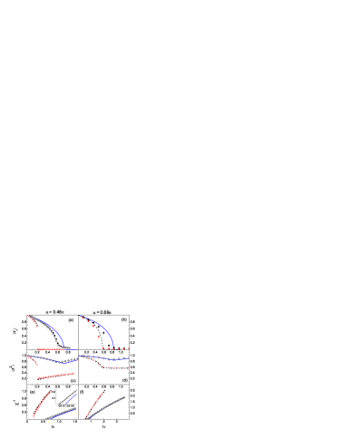
Figure 1: (Color online) (a-b) Reduced magnetization $\langle x_{z}\rangle$, (c-d) mean squared local moment $\langle x^{2}\rangle$, and (e-f) inverse paramagnetic susceptibility $\chi^{-1}$ as a function of the reduced temperature $t=T/(J_{0}m_{0}^{2})$. MFA results are shown by solid (blue online) lines for $g(x)=1$ and by dashed black lines for $g(x)=x^{-2}$. MC results are displayed by black circles for $g(x)=1$ and by red (gray) squares for $g(x)=x^{-2}$ (in both cases the symbols are filled for fcc and empty for bcc lattice). The inset in panel (e) highlights the region close to $t_{c}$ for the bcc lattice with $g(x)=1$ and also shows the results of the generalized Onsager method (black line connecting the MC points).

As seen in Fig. 1, below $T_{c}$ the average $\langle x^{2}\rangle$ declines with temperature due to the decrease of the Weiss field, which causes the maximum of the distribution function to shift to smaller moments. This is in agreement with earlier results Moriya ; Hubbard ; Hasegawa ; Uhl ; Rosengaard ; Ruban . The width of the distribution function increases with temperature, which counteracts the decrease of the local moment. The PSM with $g(x)=x^{-2}$ puts less weight on the states with large moments, and hence $\langle x^{2}\rangle$ drops much faster compared to the uniform PSM. If the Anderson criterion is not satisfied ($\alpha<\pi/2$) then the most probable moment in the paramagnetic state is zero. In this case, $\langle x^{2}\rangle$ increases with temperature above $T_{c}$ as seen in Fig. 1c. On the other hand, if the Anderson criterion is satisfied, the local moment may slightly decrease in a range of temperatures above $T_{c}$, as seen for $g(x)=x^{-2}$ in Fig. 1d.

The magnetic susceptibility above $T_{c}$ is shown in Figs. 1e,f. In MC simulations it is calculated using fluctuation-dissipation theorem, while in MFA we directly consider the response of the system to the external magnetic field. Excellent agreement between MFA and MC is observed except for the small error in $T_{c}$. In MFA one obtains above $T_{c}$

$$\chi_{\mathrm{MFA}}=\frac{\frac{1}{3}\langle x^{2}\rangle}{t-\frac{1}{3}\langle x^{2}\rangle}$$ (4)

This formula looks similar to the Curie-Weiss expression in the Heisenberg model, but here $\langle x^{2}\rangle$ depends on temperature, which leads to a renormalization of the CW constant and deviations from the CW law. The CW constant $C=d\chi^{-1}/dt$ (for a second-order phase transition) is now given by

$$C=\frac{3}{\langle x^{2}(t_{c})\rangle}\left[1-\left.\frac{d\log\langle x^{2}\rangle}{d\log t}\right|_{t_{c}}\right]$$ (5)

Thus, in addition to the usual Heisenberg term the Curie constant has a contribution due to the temperature dependence of $\langle x^{2}\rangle$ (second term in square brackets in (5)). As a result, the effective moment squared $x_{\mathrm{eff}}^{2}=3/C$ deviates from $\langle x^{2}\rangle$. As discussed above, $\langle x^{2}\rangle$ usually increases with temperature above $T_{c}$, which, according to Eq. (5), reduces $C$ and increases $x_{\mathrm{eff}}^{2}$. Moreover, for the uniform PSM $\langle x^{2}\rangle$ increases faster with temperature compared to PSM with $g(x)=x^{-2}$, and hence the CW constant is much smaller in this case (see Fig. 1f and also 1e, where the transition is however of first order).

In Fig. 2 some thermodynamic properties of the system are plotted as a function of the itinerancy parameter $\alpha$. From Eq. (4) it follows that the MFA value of $t_{c}$ for the second-order phase transision is found by solving the equation $3t_{c}=\langle x^{2}(t_{c})\rangle$, where $\langle x^{2}(t)\rangle$ is fully determined by $E(x)$ in Eq. (2). This is an easy way to estimate $T_{c}$ for an itinerant system using first-principles data for $E(x)$, $J_{0}m_{0}^{2}$, and the assumed PSM. However, for PSM with $g(x)=x^{-2}$ the transition is of first order except for a small region close to the local moment limit (in MFA the tricritical point where the order of the phase transition changes is at $\alpha_{tr}=0.632\pi$). Therefore, in general one must consider the minima of the free energy as a function of the magnetization, which can also be easily done in MFA. Note that the order of the phase transition depends on the details of the model and can change if, for example, the dependence of the exchange parameter on the magnetization is taken into account. In particular, the phase transition for the model of Ni is of first order in Ref. Uhl, (as seen from the abrupt drop of $M(T)$ and $M_{s}$ at $T_{c}$ in their Fig. 2) and in Ref. Ruban, (as seen from the abrupt drop of $\overline{m}$ in their Fig. 6), even though the uniform PSM was used in both of these models.

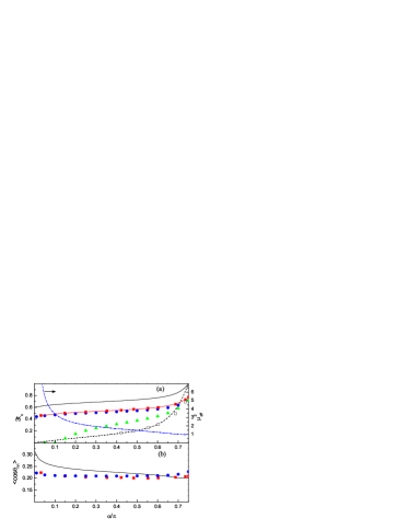
Figure 2: (Color online) (a) Reduced Curie temperature $t_{c}$ and (b) MSRO parameter $\langle\cos\theta_{nn}\rangle$ at $T=1.1T_{c}$ as a function of the itinerancy parameter $\alpha$ for the bcc lattice. Solid black line, red (gray) squares, and blue (dark gray) circles show the results of MFA, MC, and the generalized Onsager method for $g(x)=1$, respectively. Dashed black line and empty black squares depict MFA and MC results for $g(x)=x^{-2}$. Green (light gray) triangles represent the incomplete Onsager reaction field correction with the on-site interaction left unrenormalized. The blue (gray) dash-dotted line in the upper panel shows the effective moment $x^{2}_{\mathrm{eff}}$ found from the Curie constant for $g(x)=1$ in MFA. Very similar results were obtained for the fcc lattice (not shown).

From Fig. 2 we see that when the transition is of second order, MFA overestimates $T_{c}$ by about 20%, which is typical for the Heisenberg model. When the transition is of first order, MFA gives an almost exact $T_{c}$. It is important that even for the second-order transition the overestimation of $T_{c}$ in MFA does not depend on the degree of itinerancy. This is consistent with the fact that the degree of MSRO, which is shown in Fig. 2b for $T=1.1T_{c}$, is quite small and stays essentially constant in the whole range of $\alpha$. Thus, in our model itinerancy does not lead to strong short-range order. This result agrees with Refs. Rosengaard, ; Ruban, where weak short-range order was found for the models of Fe and Ni. Note that if the exchange interaction extends to more than one shell of neighbors and stays mainly ferromagnetic, the MFA validity criterion is satisfied even better, and the MSRO parameter should further decrease. Similar to the Heisenberg model, strong MSRO may only be expected in low-coordinated lattices or in the presence of frustration when for some pairs $J_{ij}/kT_{c}$ is not small.

The square of the effective moment $x^{2}_{\mathrm{eff}}$ is also shown in Fig. 2 for the uniform PSM (dash-dotted line). In the local limit $x_{\mathrm{eff}}$ naturally tends to 1. However, as $\alpha$ is decreased towards zero, the ratio $x^{2}_{\mathrm{eff}}/\langle x^{2}(t_{c})\rangle$ increases and eventually becomes much larger than 1. Similar behavior is found in functional integral theories. Moriya

IV Generalized Onsager correction for itinerant systems

Onsager introduced the concept of a cavity field in the theory of polar liquids, which is designed to go beyond the molecular field approximation (MFA) by including short-range order effects. Onsager The cavity field is the effective internal field which orients polar molecules in the ferroelectric phase. Onsager observed that each molecule polarizes the surrounding liquid and thereby generates a reaction field acting back on the molecule. However, this field is always parallel to the molecule’s dipole moment and hence does not affect its orientation. Therefore, for a liquid with permanent dipoles the reaction field must be subtracted from the mean molecular field, the result being the cavity field. Onsager also noted that the reaction field enhances the dipole moments of real molecules due to their polarizability.

The cavity field method was successfully applied to Ising Brout and Heisenberg Logan magnets which have permanent magnetic moments. Cyrot Cyrot noted that Moriya-Kawabata’s self-consistent renormalization theory for the Hubbard model may be essentially reproduced by using Onsager-like arguments; more recently this method was implemented numerically. Cyrot96 However, the actual physics there is very different; Cyrot’s approach seeks the correlation correction with respect to the Hartree-Fock solution, which is unrelated to short-range order. Onsager’s method was also applied to itinerant nickel, Staunton but, as we will see below, correct generalization to itinerant systems with LSF requires an additional ingredient which was missed in Ref. Staunton, .

We now generalize Onsager’s method to magnets with LSF described by Hamiltonian (1). Consider model (1) above $T_{c}$ in a small external collinear magnetic field $H^{ext}_{i}\mathbf{e}_{z}$. We pick site $0$ and integrate out the degrees of freedom from all the other sites in the partition function to obtain the effective Hamiltonian in the form of a generating functional for the lattice with a cavity DMFT . Expanding this functional around the atomic limit to order $1/z$ we obtain

$$H^{0}_{\mathrm{eff}}=E(m_{0})-\mathbf{m}_{0}\left(\mathbf{H}^{ext}_{0}+\sum_{i}J_{0i}\langle\mathbf{m}_{i}^{c}\rangle\right)$$

$$-\frac{m_{0}^{2}}{2}\sum_{ij}J_{0i}J_{0j}\chi_{ij}^{c}$$ (6)

where the superscript $c$ refers to the lattice with a cavity, i.e. with site $0$ removed, and we used the fluctuation-dissipation theorem to express the pair correlator through the susceptibility.

In order to find the magnetization and susceptibility of the lattice with a cavity we need to solve the “impurity problem.” Using the linked-cluster expansion technique,Wortis the longitudinal susceptibility of the original lattice can be written as follows:

$$\widehat{\chi}=\widehat{\Pi}+\widehat{\Pi}\widehat{W}\widehat{\Pi}$$ (7)

where $\widehat{W}$ is the effective interaction that satisfies the equation $\widehat{W}=\widehat{J}+\widehat{J}\widehat{\Pi}\widehat{W}$, and $\widehat{\Pi}$ is the 1-bond-irreducible “polarization operator” which may be shown to be local to first order in $1/z$. VLP (All quantities in Eq. (7) are matrices in site indices.) Removal of site $0$ may be formally represented by a perturbation $\Delta\widehat{\Pi}=-\Pi_{00}\delta_{0i}\delta_{0j}$ to $\widehat{\Pi}$. (The renormalization of $\Pi_{jj}$ for $j\neq 0$ due to removal of site $0$ is at least of order $1/z^{2}$.) Thus, denoting the effective interaction matrix for the cavity lattice as $\widehat{W}_{c}$, we may write $\widehat{W}_{c}^{-1}-\widehat{W}^{-1}=-\Delta\widehat{\Pi}$. Using (7) and the fact that $\widehat{\Pi}$ is diagonal, we find

$$\chi^{c}_{ij}=\chi_{ij}-\frac{\chi_{i0}\chi_{0j}}{\chi_{00}}.$$ (8)

The average local moments $\mathbf{M}^{c}_{i}=\langle\mathbf{m}^{c}_{i}\rangle$ for the lattice with a cavity are:

$$M_{i}^{c}=\sum_{j}\chi^{c}_{ij}H^{ext}_{j}=M_{i}-\frac{\chi_{i0}}{\chi_{00}}M_{0},$$ (9)

where $M_{i}$ are the average local moments of the complete lattice without the cavity. The value of $\mathbf{H}^{ext}_{0}$ does not affect $M_{i}^{c}$ (as expected), therefore in the right-hand side of (9) we may take $M_{i}$ and $M_{0}$ for the actual field distribution.

From the effective Hamiltonian (6) we can find the magnetization at site $0$:

$$M_{0}=\tilde{\chi}^{0}\tilde{H}_{W}$$ (10)

where

$$\tilde{H}_{W}=H^{ext}_{0}+\sum_{i}J_{0i}\left(M_{i}-\frac{\chi_{i0}}{\chi_{00}}M_{0}\right)$$ (11)

is the renormalized effective field (cavity field), and $\tilde{\chi}^{0}$ is the renormalized bare (atomic-limit) susceptibility. The latter may be written as $\tilde{\chi}^{0}=\langle m^{2}\rangle_{\lambda}/3T$, where the average paramagnetic squared local moment $\langle m^{2}\rangle_{\lambda}$ is calculated using a renormalized on-site exchange $\widetilde{I}=I+\lambda$ with $\lambda=\sum_{ij}J_{0i}J_{0j}\chi_{ij}^{c}$. This renormalization of the bare susceptibility is the essential ingredient needed to extend Onsager’s theory to itinerant magnets. It has no effect in the localized limit where $m^{2}$ is constant.

As usual, we now obtain the Fourier transform of the susceptibility:

$$\chi_{\mathbf{q}}=\frac{\tilde{\chi}^{0}}{1-\tilde{\chi}^{0}(J_{\mathbf{q}}-\lambda)}\;,$$ (12)

where $\lambda=\sum_{\mathbf{q}}J_{\mathbf{q}}\chi_{\mathbf{q}}/\chi_{00}$. We used the same symbol $\lambda$ as above in the definition of $\widetilde{I}$, because these expressions are identical, as can now be shown with the help of Eqs. (12) and (8). Eq. (12) with the definitions of $\lambda$, $\tilde{\chi}^{0}$ and $\widetilde{I}$ form a closed set of equations for the paramagnetic susceptibility. Note that (12) automatically leads to a sum rule $\chi_{00}=\tilde{\chi}^{0}$, which agrees with the fluctuation-dissipation theorem.

At the Curie temperature $\chi_{\mathbf{q}}$ diverges at $\mathbf{q}=0$. Therefore, from (12) we obtain $T_{c}=\frac{1}{3}J_{0}\langle m^{2}(T_{c})\rangle_{\lambda}/G$, where $G=\sum_{\mathbf{q}}(1-J_{\mathbf{q}}/J_{0})^{-1}$ is the diagonal element of the lattice Green’s function. Logan Note that the value of $\lambda$ at $T_{c}$ is equal to $J_{0}(1-G^{-1})$ and independent of the degree of itinerancy $\alpha$.

The reduced Curie temperature $t_{c}$ and MSRO parameter $\langle\cos\theta_{nn}\rangle$ at $T=1.1T_{c}$ calculated in this way are shown in Fig. 2 for the bcc lattice and the PSM with $g(x)=1$. The agreement with MC results is excellent in the whole range of $\alpha$. We repeated these calculations for the fcc lattice and found excellent agreement with MC as well. The accuracy of the predicted $t_{c}$ may be seen from Table 1. Similar performance for bcc and fcc lattices suggests that this approximation is not very sensitive to the connectivity of the lattice. The paramagnetic susceptibility is also shown in Fig. 1e for $\alpha=0.48\pi$, bcc lattice, and uniform PSM. The agreement with MC results is essentially perfect outside of the narrow critical region.

Table 1: Reduced Curie temperature $t_{c}$ for bcc and fcc lattices for PSM with $g(x)=1$: Results of the mean-field approximation (MFA), Horwitz-Callen approximation (HC), generalized Onsager method (GO) and Monte Carlo (MC).

$\alpha/\pi$	bcc				fcc
	MFA	HC	GO	MC	MFA	HC	GO	MC
0.032	0.621	0.449	0.451	0.462(1)	0.621	0.465	0.466	0.480(2)
0.148	0.660	0.484	0.486	0.504(2)	0.660	0.501	0.502	0.520(5)
0.250	0.681	0.503	0.504	0.525(2)	0.681	0.519	0.520	0.540(5)
0.352	0.699	0.518	0.520	0.543(2)	0.699	0.535	0.536	0.562(2)
0.422	0.712	0.529	0.530	0.553(1)	0.712	0.546	0.547	0.570(5)
0.483	0.723	0.539	0.541	0.568(1)	0.723	0.557	0.558	0.584(2)
0.553	0.745	0.555	0.557	0.585(2)	0.745	0.572	0.574	0.600(1)
0.602	0.765	0.570	0.573	0.600(2)	0.765	0.589	0.590	0.617(2)
0.687	0.834	0.619	0.622	0.654(3)	0.834	0.640	0.642	0.672(6)
0.735	0.942	0.683	0.688	0.732(2)	0.942	0.708	0.711	0.753(6)
0.750	1	0.713	0.718	0.770MCheisenberg	1	0.740	0.743	0.788(3)

The first-order terms in the $1/z$ expansion derived above introduce two corrections to MFA. The first one is the subtracted mean reaction field; this correction reduces the magnetization. This is the only correction in Onsager’s method for systems with permanent moments. The second correction described by the last term in Eq. (6) adds back the fluctuating reaction field which is always parallel to the moment on the central site. For the Heisenberg (or Ising) model this second correction has no effect, but in itinerant systems it always increases the local moments and hence the Curie temperature. There is a strong cancelation between these two corrections in itinerant systems, and improvement compared to MFA may be achieved only if both of them are included. Indeed, if the renormalization of the Stoner parameter is not taken into account (i.e. if the last term in Eq. (6) is dropped), we find a spurious strong suppression of $T_{c}$ for itinerant systems, as shown in Fig. 2a.

It is interesting to compare the generalized Onsager method with the Horwitz-Callen (HC) approximation which is based on the “ring subset” of diagrams for the generating functional $\Phi$ in the linked-cluster technique.HC ; Wortis In this method, the second-order self-field $G_{2}$ is found by differentiating $\Phi$ with respect to the renormalized second cumulant $M_{2}$, while $M_{2}$ is represented by an integral containing $G_{2}$ as a parameter. This technique does not assume any particular form for the atomic limit, and therefore it can be used in our case including LSF as well. In the HC method, the on-site correlator may be found as $K_{00}=M_{2}+2M_{2}^{2}G_{2}$, and the sum rule $K_{00}=1$ is not satisfied in the paramagnetic Heisenberg magnet. However, it is easy to check that the value of $K_{00}$ at $T_{c}$ is smaller than 1 by less than a percent in bcc and fcc lattices. In Onsager’s method for the Heisenberg model, the sum rule $K_{00}=1$ is used to fix $M_{2}$ instead of the integral representation as in the HC method. The results for $T_{c}$ are therefore very close. We found that this close similarity remains in the entire range of $\alpha$, as seen from Table 1. The generalized Onsager’s method is, however, technically much simpler.

V Conclusions

We have studied the thermodynamics of a simple classical spin fluctuation model allowing for a variable degree of itinerancy. This model is qualitatively similar to those used before to study the thermodynamics of Fe and Ni using first-principles data. Uhl ; Rosengaard ; Ruban It is worth emphasizing that the main drawback of using classical spin models of this type is the ambiguity of the phase space measure. As we showed above, the thermodynamics is very sensitive to this measure for systems with even intermediate degree of itinerancy. While the energetics of constrained spin configurations may, at least in principle, be accurately mapped using DFT calculations, it is not known (to our knowledge) how and whether the phase space measure can be supplied in a realistic way.

In the present work, we focused on the general features of the model rather than on the determination of its parameters from principles. We found that the thermodynamic properties are similar to the results of the functional integral approach. Moriya ; MT78 ; Hubbard ; Hasegawa Further, we found that the mean-field approximation is qualitatively valid, and short-range order is weak and almost independent on the degree of itinerancy up to the strongly itinerant limit where the paramagnetic susceptibility is dominated by longitudinal fluctuations. This is in agreement with earlier results for the models of Fe and Ni; Rosengaard ; Ruban it is clear that this is a general feature of the classical model with no frustration.

Further, we generalized the Onsager cavity field method to itinerant systems using an expansion around the atomic limit to first order in $1/z$. Both the interatomic exchange constant and the Stoner parameter are renormalized by short-range order. When both these corrections are included, the Curie temperature is in excellent agreement with Monte Carlo results. However, simple subtraction of the Onsager reaction field is a very poor approximation.

- (1) T. Moriya, Spin fluctuations in itinerant electron magnetism (Springer, Berlin, 1985).
- (2) K. K. Murata and S. Doniach, Phys. Rev. Lett. 29, 285 (1972).
- (3) G. G. Lonzarich and L. Taillefer, J. Phys. C 18, 4339 (1985).
- (4) T. Moriya and Y. Takahashi, J. Phys. Soc. Japan 45, 397 (1978).
- (5) J. Hubbard, in: Electron correlation and magnetism in narrow-band systems, ed. by T. Moriya (Springer, Berlin, 1981), p. 29.
- (6) H. Hasegawa, ibid., p. 38.
- (7) L. D. Landau and E. M. Lifshitz, Statistical Physics (Pergamon, Oxford, 1980), sec. 147.
- (8) P. Mohn and E. P. Wohlfarth, J. Phys. F 17, 2421 (1986).
- (9) R. F. Hassing and D. M. Esterling, Phys. Rev. B 7, 432 (1973).
- (10) B. L. Gyorffy, A. J. Pindor, J. Staunton, G. M. Stocks, and H. Winter, J. Phys. F: Met. Phys. 15, 1337 (1985).
- (11) P. H. Dederichs, S. Blügel, R. Zeller, and H. Akai, Phys. Rev. Lett. 53, 2512 (1984).
- (12) T. Oguchi, K. Terakura, and N. Hamada, J. Phys. F 13, 145 (1983).
- (13) J. B. Staunton and B. L. Gyorffy, Phys. Rev. Lett. 69, 371 (1992).
- (14) M. Uhl and J. Kübler, Phys. Rev. Lett. 77, 334 (1996).
- (15) N. M. Rosengaard and B. Johansson, Phys. Rev. B 55, 14975 (1997).
- (16) M. Lezǎić, P. Mavropoulos, J. Enkovaara, G. Bihlmayer, and S. Blügel, Phys. Rev. Lett. 97, 026404 (2006)
- (17) A. V. Ruban, S. Khmelevskyi, P. Mohn, and B. Johansson, Phys. Rev. B 75, 054402 (2007).
- (18) A. Georges, G. Kotliar, W. Krauth, and M. J. Rozenberg, Rev. Mod. Phys. 68, 13 (1996).
- (19) V. P. Antropov, Phys. Rev. B 72, 140406(R) (2005).
- (20) J. Kübler, J. Phys.: Condens. Matter 18, 9795 (2006).
- (21) We are grateful to V. P. Antropov for his suggestion that the Anderson criterion can be used to quantify the degree of itinerancy.
- (22) D. P. Landau, K. Binder, A guide to Monte Carlo simulations in Statistical Physics, (Cambridge University Press, Cambridge, 2000).
- (23) L. Onsager, J. Am. Chem. Soc. 58, 1486 (1936).
- (24) R. Brout and H. Thomas, Physics (Long Island City, N.Y.) 3, 317 (1967).
- (25) D. E. Logan, Y. H. Szczech, and M. A. Tusch, Europhys. Lett. 30, 307 (1995).
- (26) M. Cyrot, in: Electron correlation and magnetism in narrow-band systems, ed. by T. Moriya (Springer, Berlin, 1981); J. Magn. Magn. Mater. 45, 9 (1984).
- (27) M. Cyrot and H. Kaga, Phys. Rev. Lett. 77, 5134 (1996); H. Kaga and M. Cyrot, Phys. Rev. B 58, 12267 (1998).
- (28) M. Wortis, in Phase Transitions and Critical Phenomena, Vol. 3, ed. by C. Domb and M. S. Green (Academic, London, 1974), p. 114.
- (29) V. G. Vaks, A. I. Larkin, and S. A. Pikin, Sov. Phys. – JETP 24, 240 (1967) [Zh. Eksp. Teor. Fiz. 51, 361 (1966)].
- (30) G. Horwitz, H. B. Callen, Phys. Rev. 124, 1757 (1961).
- (31) K. Chen, A. M. Ferrenberg, D. P. Landau, Phys. Rev. B 48, 3249 (1993).