Geometric Scaling of $F_{2}$ and $F_{2}^{c}$ in data and QCD Parametrisations

Abstract

The scaling properties at low $x$ of the proton DIS cross section and its charm component are analyzed with the help of the quality factor method. Scaling properties are tested both in the deep inelastic scattering data and in the structure functions reconstructed from CTEQ, MRST and GRV parametrisations of parton density functions. The results for DIS cross sections are fully compatible between data and parametrisations. Even with larger error bars, the charm component data favors the same geometric scaling properties as the ones of inclusive DIS. This is not the case for all parametrisations of the charm component.

I Introduction

Geometric scaling Stasto:2000er is a remarkable empirical property verified by data on high energy deep inelastic scattering (DIS) $i.e.$ virtual photon-proton cross-sections. One can indeed represent with reasonable accuracy the cross section $\sigma^{\gamma^{*}p}$ in the low Bjorken $x$ regime by the formula

$$\sigma^{\gamma^{*}p}(x,Q)=\sigma^{\gamma^{*}}(\tau)\ ,\quad\textrm{where}\quad\tau=\log\left(\frac{Q^{2}}{Q_{s}^{2}(Y)}\right)$$ (1)

is the scaling variable, $Q$ the virtuality of the photon, and $Y\equiv\log(1/x)$ the total rapidity in the ${\gamma^{*}}$-proton system. That empirical property is often considered as a hint for gluon saturation effects. Indeed, including non-linear effects due to high parton density in the evolution equations for parton distributions towards low $x$ leads to such geometric scaling properties. In that context, $Q_{s}(Y)$ is called the saturation scale, and gives the typical scale for the onset of nonlinear effects. Using the dipole factorization of DIS observables, one predicts geometric scaling to hold also for deeply virtual Compton scattering, exclusive vector meson production and inclusive diffraction, which has been verified empirically Marquet:2006jb . Several types of geometric scaling or of generalizations of geometric scaling have been proposed in the literature, which correponds to various sets of approximations in the theoretical description of parton evolution and gluon saturation.

The quality factor (QF) introduced in usgeom is an interesting tool in order to discuss scaling properties. It allows to compare the validity of different scaling laws on a given data set, without any assumption concerning the shape of the scaling function. It has been used in usgeom ; usscaling in order to study the above-mentioned scaling properties in the data for DIS observables. A standard fit to data tests locally in each bin the value of an observable, whereas the QF only considers point-to-point correlations for the observable. Hence, the QF method could give complementary informations, difficult to catch with a standard fit if the data are not very precise. For that reason, it is interesting to test with the QF method to what extend global fits to parton distribution functions (PDF) leads to the same scaling properties as the data. Many efforts have been made in the last few years by the MRST and CTEQ groups in order to implement heavy quark mass effects in a consistent way in their global fits. That justifies the comparison of data and PDF sets not only for the inclusive DIS cross section $\sigma\sim F_{2}/Q^{2}$ but also for its charm component $\sigma^{c}\sim F_{2}^{c}/Q^{2}$. The data for the bottom component $F_{2}^{b}/Q^{2}$ are not suitable for a scaling analysis, since they contain too few points.

The plan of the paper is as follows. In section II we review recent improvements in the treatment of heavy flavors in PDF’s global fits, and we present the PDF sets used in the present study. In section III we describe the various scaling hypotheses to be tested and their theoretical motivation. In section IV we present the Quality Factor method we shall use in the analysis and the set of data we consider for the fitting procedure. We provide and comment our results for $F_{2}$ in section V and for $F_{2}^{c}$ in section VI. The section VII is devoted to the summary and the discussion of the results.

II PDFs with heavy quark mass effects

Let us briefly discuss the recent progresses concerning the treatment of heavy quark mass effects in PDFs global fits. In the collinear factorization framework, one factorizes observables (e.g. proton structure functions) as a convolution of coefficient functions, describing partonic matrix elements, and PDFs for active flavors. In that formalism, active flavors are massless. Thus it should be relevant only if the quark masses corresponding to active flavors are small compared to the factorization scale $\mu_{F}$, usually chosen to be a hard scale of the problem, such as $Q$ for DIS. The most standard pQCD scheme for heavy flavors is the fixed flavor number scheme (FFNS), where heavy flavors are not considered as active, and are generated only by boson-gluon fusion. It gives reliable results for $Q=\mu_{F}$ of the order of the heavy quark mass $m_{hf}$. However, for $Q^{2}\gg m_{hf}^{2}$ higher order terms in the coefficient functions are enhanced by powers of $\log(Q^{2}/m_{hf}^{2})$, so that perturbation theory breaks down. In order to overcome this difficulty, variable flavor number schemes (VFNS) have been introduced. They consist in a succession of FFNS with one additional active flavor each time $Q$ becomes larger than the mass of a heavy quark flavor. Two successive FFNS are matched with each other at the value $Q^{2}\simeq m_{hf}^{2}$ chosen for the change of scheme, in order to ensure that renormalization is done in a consistent way for all FFNS. In the the first implementations of VFNS, called zero-mass-VFNS (ZM-VFNS), the switching from one FFNS to another at $Q^{2}\simeq m_{hf}^{2}$, which is an unphysical change of factorization scheme, was coinciding with the threshold of production of the heavy flavor in the final state. That is not considered to be correct, and the latter should correspond to a threshold in the total energy $W$ rather than in $Q$. That difficulty and a few others are solved if one goes to the general-mass-VFNS (GM-VFNS), build in Collins . One of the ingredients used in the GM-VFNS is the replacement of $x$ by the rescaled variable

$$\chi=x\left(1+\frac{4m_{hf}^{2}}{Q^{2}}\right)$$ (2)

when a pair of heavy quarks $H\bar{H}$ is produced in the final state, in order to ensure the right kinematical threshold: for $W$ as small as $2m_{hf}$, $\chi$ goes to $1$ and thus the cross section for heavy quark pair production vanishes.

The recent global fits of PDFs of the CTEQ and MRST groups are using such GM-VFNS. However, the details of the implementation differs between the two groups Tung:2006tb ; Thorne:2006qt . In particular, they use different conventions to name the order of the analysis (see e.g. Thorne:2008xf ), such as LO, NLO, etc. In our study, we use the following general purpose GM-VFNS PDFs sets: the NLO CTEQ6.6M Nadolsky:2008zw , the NNLO MRST2006 Martin:2007bv , and the NLO MRST2004 Martin:2004ir . We consider also the NNLO MRST2004 Martin:2004ir , which only uses an approximate implementation of GM-VFNS, and the older GRV98 Gluck:1998xa PDFs set based on a FFNS with 3 flavors.

In all of the abovementioned parametrisations, the charm production in DIS appears only pertubatively and the charm and anticharm PDFs (if any) start from zero at an intial factorization scale below the charm mass. Alternatively, some theoretical models for the nucleon content feature a non-perturbative intrinsic charm component. The CTEQ group studied that possibility, and released the PDFs sets CTEQ6.6C1 to CTEQ6.6C4 Nadolsky:2008zw , which extend CTEQ6.6M by including various types of intrinsic charm component. The CTEQ6.6C1 and CTEQ6.6C2 parametrisations correspond respectively to a moderate and a strong intrinsic charm contribution of the form predicted by the BHPS model Brodsky:1980pb , which is non-negligible only at large x. By contrast, the CTEQ6.6C3 and CTEQ6.6C4 parametrisations correspond respectively to a moderate and a strong intrinsic charm contribution proportional to the light sea quark contribution at the initial scale for the global fit. They are not motivated by theoretical models.

III Scaling Variables from saturation physics

Let us sketch the theoretical motivation for the different forms of scaling (see TABLE I) proposed for deep-inelastic scattering at high energy. The evolution of unintegrated parton densities towards large rapidity $Y$ at fixed $k_{T}^{2}$ is given by the BFKL Lipatov:1976zz equation, provided that these unintegrated parton densities are small. Generic solutions of that linear evolution can be written as a sum of elementary wave solutions, with the help of Mellin transform. Each of these elementary wave solutions have scaling properties, but generically not their superposition. However, the BFKL evolution in $Y$ leads to larger and larger unintegrated gluon density due to soft gluon radiation. At some point, the partons are so packed that additional soft gluons are emitted collectively. Thus, the soft gluons radiation is reduced by destructive interferences and the evolution becomes nonlinear in domain typically given by $k_{T}<Q_{s}(Y)$. The BFKL equation is then generalized e.g. by the BK Balitsky:1995ub or JIMWLK JIMWLK nonlinear equations. For a review about that gluon saturation phenomenon, see Iancu:2003xm . Such a nonlinear evolution equation has the following property. Even in the kinematical domain in which the nonlinear terms are negligible compared to the linear ones, the nonlinearity of the equation constrains the solution, acting as a dynamical boundary condition to the linear BFKL evolution Mueller:2002zm . The interplay between that specific boundary condition and the BFKL kernel selects dynamically Munier:2003vc a specific wave solution (the critical one) of the BFKL equation in a window $k_{T}^{2}\gtrsim Q_{s}(Y)$, which determines the evolution of $Q_{s}(Y)$. In that kinematical range, the solution of the nonlinear evolution loses memory of the initial condition. Hence, one finds that the unintegrated gluon distribution scales with $k_{T}^{2}/Q_{s}(Y)$ above the saturation scale. Due to the $k_{T}$-factorization in the linear regime, that property result in a geometric scaling (1) of the DIS cross-section, and of other observables.

In a fixed coupling $\alpha_{s}$ approximation, that mechanism is well understood, and leads to a saturation scale $\log Q_{s}(Y)\sim\lambda Y$. This corresponds to the geometric scaling variable FC in TABLE I. If one goes to the running coupling case, the mechanism leading to the scaling holds, but is analytically under control only at large enough $Q^{2}$, due to asymptotic freedom. One can deduce only the large $Y$ behavior of the saturation scale, which is $\log Q_{s}(Y)\sim\lambda\sqrt{Y}$. Thus, one gets the predicted scaling property at large $Y$ and $Q^{2}$ (with $\log Q^{2}\propto\sqrt{Y}$). However, the extrapolation of that scaling property towards the finite $Q^{2}$ and $Y$ phenomenologically relevant domain is not unique. We consider in particular two different scaling variables, which both give the theoretical asymptotic behavior. The first one is a genuine geometric scaling variable (as defined in (1)). It is called RCI in TABLE I. The second scaling variable gb compatible with the asymptotic prediction is given in TABLE I and called RCII. Its value for the parameter $\lambda$ should be the square of the one for the RCI scaling. In the recent years, the possible impact on saturation of fluctuations due e.g. to Pomeron loops has been extensively discussed. They lead to a random saturation scale, but event-by-event the geometric scaling property is preserved. In the fixed coupling approximation, the distribution of $\log Q_{s}^{2}(Y)$ is approximately gaussian, with a variance proportionnal to $Y$. Finally, one expect the cross section to scale with the diffusive scaling variable Hatta:2006hs (DS in TABLE I) which is the original geometric scaling variable divided by the dispersion $\sqrt{Y}$.

IV The Quality factor method

In this section, we remind briefly the definition of the Quality Factor ($QF$) which we use to compare quantitatively the different scaling variables (see Table 1). We already used this method to compare the scaling results for the proton structure function $F_{2}$, the deeply virtual Compton scattering (DVCS), the diffractive structure function, and the exclusive vector meson production data measured at HERA usscaling .

Given a set of data points $(Q^{2},x,\sigma=\sigma(Q^{2},x))$ and a parametric scaling variable $\tau=\tau(Q^{2},Y=\log(1/x);\lambda)$ we want to know whether the cross-section can be parametrised as a function of the variable $\tau$ only. Since the function of $\tau$ that describes the data is not known, the $QF$ has to be defined independently of the form of that function. The $QF$ allows to quantitatively describe whether pairs of $\sigma=\sigma(Q^{2},x)$ and $\tau=\tau(Q^{2},Y=\log(1/x);\lambda)$ lie on a single curve for a given parameter $\lambda$.

For a set of points $(u_{i},v_{i})$, where $u_{i}$’s are ordered, we introduce $QF$ as follows usgeom

$$QF(\lambda)=\biggl{[}\sum_{i}\frac{(v_{i}-v_{i-1})^{2}}{(u_{i}-u_{i-1})^{2}+\epsilon^{2}}\biggr{]}^{-1},$$ (3)

where $\epsilon$ is a small constant that prevents the sum from being infinite in case of two points have the same value of $u$. According to this definition, the contribution to the sum in (3) is large when two successive points are close in $u$ and far in $v$. Therefore, a set of points lying close to a unique curve is expected to have larger $QF$ (smaller sum in (3)) compared to a situation where the points are more scattered.

Since the cross-section in data differs by orders of magnitude and $\tau$ is more or less linear in $\log(Q^{2})$ (see Table 1), we decided to take $u_{i}=\tau_{i}(\lambda)$ and $v_{i}=\log(\sigma_{i})$. This ensures that low $Q^{2}$ data points contribute to the $QF$ with a similar weight as higher $Q^{2}$ data points. The set $(u_{i},v_{i})$ has to be ordered in $u$ before entering the $QF$ formula. In order to stay independent of the exact values of $u$ and $v$, all the values are rescaled so that $0\leq u_{i},v_{i}\leq 1$. All the $QF$’s in this Letter are calculated with $\epsilon=0.01$.

In order to test a scaling law $\tau$ and say whether the points $(\sigma_{i},\tau_{i})$ lie on a single line or not, we search for the parameter $\lambda$ that minimises the $1/QF$ variable. The minimum value of $1/QF$ is obtained using the MINUIT package. Given the maximum value of the $QF$ (minimum of $1/QF$), we are able to directly compare different scaling laws.

	scaling	$\tau$ formula	parameters
FC	“Fixed Coupling”	$\log Q^{2}-\lambda Y$	$\lambda$
RCI	“Running Coupling I”	$\log Q^{2}-\lambda\sqrt{Y}$	$\lambda$
RCII	“Running Coupling II”	$\log(Q^{2}/\Lambda^{2})-\lambda\frac{Y}{\log(Q^{2}/\Lambda^{2})}$	$\lambda$
			$\Lambda=$0.2 GeV
DS	“Diffusive Scaling”	$\frac{\log(Q^{2}/\Lambda^{2})-\lambda Y}{\sqrt{Y}}$	$\lambda$
			$\Lambda=$1 GeV

Table 1: Scaling variables used in the fits to deep inelastic scattering data usscaling .

In this Letter, we aim to extend the study performed in Ref. usscaling by considering the different $F_{2}$ parametrisations and the proton charm structure function data $F_{2}^{c}$ measured at HERA and given by different parametrisations.

V Fits to inclusive DIS

We first aim to test the scaling quality using parametrisations of the proton structure function $F_{2}$ using the parametrisations from the CTEQ, MRSTW and GRV groups discussed in section II.

In a previous paper usscaling , we tested the scaling properties of $F_{2}/Q^{2}$ using the data available from the H1 H1 , ZEUS ZEUS , NMC NMC and E665 E665 experiments. We follow the same kinematical cuts for the parametrisations as we used for the experimental data usscaling . We only consider data with $x<10^{-2}$ and $Q^{2}$ in the range $[3;150]$ GeV². The points with $x>10^{-2}$ are removed from the data since valence quark densities dominate here, and the formalism of saturation cannot apply in this kinematical region. Similarly, the upper $Q^{2}$ cut is introduced, while the lower $Q^{2}$ cut ensures that we stay away from the soft QCD domain. In this kinematical domain, 217 data points are used. In order to be able to directly compare scaling properties in the CTEQ, MRST and GRV parametrisations to the experimental data, we choose the same 217 pairs of $x$ and $Q^{2}$ as in data.

The $QF$ method is more likely to prefer the parametrisations over data, since there is no statistical fluctuation in the parametrisations, contrary to data. It becomes clear from the definition that the statistically scattered values of structure functions in the experimental data lead to worse $QF$ than a smooth parametrisation. In this sense, we cannot use the value of the $QF$ to compare the scaling properties between experimental data and parametrisations. However, the $QF$ can be directly compared among different parametrisations and can also test the differences among scaling laws tested on one particular data set.

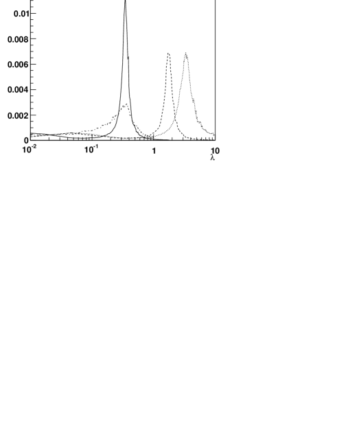
Figure 1: Different scalings for $F_{2}/Q^{2}$ measured data and the CTEQ6.6M parametrisation for $Q^{2}>3$ GeV²: Upper curves: Scaling curve for “Fixed Coupling” (left) and $QF$ against $\lambda$ for different scalings laws in data (right). Lower curves: same studies for the CTEQ6.6M parametrisation. Results are found similar for the different CTEQ, GRV and MRST parametrisations and are similar to data.

Table 2 shows the fit results for all data and the parametrisations. Similarly as in data, the MRST and GRV parametrisations give similar $QF$ for fixed coupling, running coupling I and running couping II. On the contrary, CTEQ favours fixed coupling. All parametrisations disfavour diffusive scaling, and all $\lambda$ values are consistent among different data sets. We can also see that GRV leads to smaller values of $QF$ than MRST and CTEQ, but all parametrisations lead to a good $QF$. Scaling curves and fit results for experimental data and the CTEQ6.6M parametrisation, as an example, are shown in figure 1.

We note that the CTEQ, MRST and GRV parametrisations of the data lead to good scalings, whereas they do not contain any saturation hypothesis. One may wonder if such result comes from the chosen form of the parametrisation at the initial scale $Q_{0}$, or if DGLAP evolution itself leads to a scaling in the HERA kinematical range.

VI Fits to the charm component of DIS

In a second part of the paper, we want to study the scaling properties of the charm component of the structure function $F_{2}^{c}/Q^{2}$, both in data and in parametrisations.

VI.1 Fits to $F_{2}^{c}/Q^{2}$ in data and parametrisations

First we test the scaling properties using experimental data. The requirements on the kinematical domain remain the same as in the previous section. Now the lower $Q^{2}>3$ GeV² cut also allows to remove a part of the charm mass effects. We use the charm $F_{2}^{c}$ measurements from the H1, ZEUS and EMC experiments charm . Only 25 data points lie in the kinematical region we want to analyse.

Since the statistics in the data is low, the fit results are not precise. Nevertheless, they still lead to clear results that are comparable to $F_{2}$ fits. Table III shows the results of the fits to the $F_{2}^{c}$ data for different scaling laws. The results are found similar between $F_{2}$ and $F_{2}^{c}$ (see Fig. 2, top left plot). All $\lambda$ parameters are similar except for Diffusive Scaling. As in the case of the $F_{2}$ scaling analysis usscaling , Fixed Coupling, Running Coupling I and Running Coupling II give similar values of $QF$, and Diffusive Scaling is disfavoured.

It is now interesting to check whether the scaling properties are also observed using the $F_{2}^{c}$ parametrisation of the data, as seen in the previous section for the proton structure functions $F_{2}$. The results are given in Table III and Fig. 2. Fig. 2 displays the values of the $QF$ for Fixed Coupling and different parametrisations. The value of $\lambda$ favoured by the GRV and MRST parametrisations has a tendency to be larger (about 1) than the value favoured in data (about 0.3). It is worth noticing however that the data show a smaller peak in the $QF$ distribution around 1 as well which is disfavoured, and the MRST parametrisation another peak towards 0.3. The CTEQ parametrisation is definitely closer to the results in data leading to a value of $\lambda$ close to 0.5 for the CTEQ6.6M NLO parametrisation, and to 0.4 when one introduces an additional sea-like intrinsic charm contribution (CTEQ6.6C3 and CTEQ6.6C4). The results for the different scalings are given in Table III, and the conclusion remains unchanged.

Let us now summarize what we obtained comparing data and simulation of $F_{2}^{c}$. First of all, the value of $\lambda$ favoured in data is compatible with the one obtained for $F_{2}$, DVCS… Of course the value of $\lambda$ shows a large error bar since the number of data points is only 25, but it is quite striking that the same value as for $F_{2}$ is found. Everything looks as if the charm quark was behaving like any other light quark from the point of view of scaling. New data on $F_{2}^{c}$ which will be published soon by the H1 and ZEUS collaborations are of great interest. The MRST and GRV parametrisations favour different values of $\lambda$ while the CTEQ ones are compatible with data, especially when an instrinsic charm component is added.

The next step of our study relies more in understanding in more detail the differences between the parametrisations, since we recall that they lead to a good description of $F_{2}^{c}$ itself.

VI.2 Comparison between different $F_{2}^{c}$ parametrisations

Taking the same 25 points as in data is not sufficient to investigate differences among the parametrisations. In order to analyse the parametrisations in detail, we choose to use the same $x$ and $Q^{2}$ as for $F_{2}$ which leads to 217 points.

The results for the 217 points are given in Table 4 for the CTEQ parametrisation. For the sake of clarity, we choose to perform the study for Fixed Coupling geometric scaling only — the differences among different scaling laws are not large and do not modify the conclusion of the study. We note that scaling is indeed obtained in the different CTEQ parametrisations, and the value of $\lambda$ which maximises $QF$ is compatible with the value measured in data. The CTEQ6.6C4 parametrisation, which has a strong sea-like intrinsic charm contribution, gives the $\lambda$ value that is closest to $\lambda=0.3$ found in data and leads to a much better $QF$ than the other parametrisations. It is also worth noticing that the values of $\lambda$ are quite stable for different $Q^{2}$ cuts.

A new striking result appear with the MRST and GRV parametrisations when one uses 217 points. The MRST 2006 NNLO and the MRST 2004 NLO and NNLO parametrisations, as well as the GRV98 one, do not show any scaling at all. No value of $\lambda$ that maximises $QF$ is found within an acceptable range. We now study the behaviour of the MRST and GRV parametrisations after different cuts on $Q^{2}$. Increasing the cut to 5 GeV² does not help, therefore we choose to study the effects of higher $Q^{2}$ cuts. Table 5 gives the fit results in three different $Q^{2}$ ranges, namely $[10;150]$, $[15;150]$ and $[25;150]$ GeV². Scaling properties are not observed using the MRST parametrisations even in the $Q^{2}$ range $[10;150]$ GeV². The values of $QF$ are much smaller than the ones obtained with CTEQ (see Table 5). However, geometric scaling appears at higher $Q^{2}$ and the value of $\lambda\sim 0.65$. The situation for the GRV98 parametrisation is found to be similar as for MRST, but leading to a higher value of $\lambda$.

As a conclusion to this second study, it looks like the MRST, GRV and CTEQ parametrisations of $F_{2}^{c}$ show a different behaviour from the scaling point of view. While the CTEQ parametrisation shows a scaling even at lower $Q^{2}$ (which seems observed in data), the MRST parametrisation only shows scaling at higher $Q^{2}$. Further more, the GRV parametrisation leads to a much higher value of $\lambda$ than the one favoured in data. This difference might be due to the different forms of the gluon distribution at the initial scale $Q_{0}^{2}$ chosen by the CTEQ and MRST groups. It will be worth to test this further using new measurements of $F_{2}^{c}$ which should be available soon.

Finally, let us mention that we have checked that substitution in the scaling formulae of $x$ by the rescaled variable $\chi$ (see Formula (2)) used in the GM-VFNS has a negligible effect in the considered kinematical ranges and does not change our results and conclusions.

data set	FC	RC I	RC II	DS
data	$\lambda$=0.33	$\lambda$=1.84	$\lambda$=3.44	$\lambda$=0.36
	$QF$=1.63	$QF$=1.62	$QF$=1.69	$QF$=1.44
GRV98	$\lambda$=0.33	$\lambda$=1.87	$\lambda$=3.35	$\lambda$=0.37
	$QF$=5.5	$QF$=5.2	$QF$=4.8	$QF$=3.7
MRST 2004 NLO	$\lambda$=0.34	$\lambda$=1.72	$\lambda$=3.31	$\lambda$=0.31
	$QF$=11.3	$QF$=9.6	$QF$=7.2	$QF$=4.4
MRST 2004 NNLO	$\lambda$=0.34	$\lambda$=1.72	$\lambda$=3.30	$\lambda$=0.36
	$QF$=11.2	$QF$=11.3	$QF$=7.6	$QF$=4.3
CTEQ 6.6 M	$\lambda$=0.35	$\lambda$=1.84	$\lambda$=3.40	$\lambda$=0.38
	$QF$=12.4	$QF$=6.6	$QF$=6.4	$QF$=2.7
CTEQ 6.6 C1	$\lambda$=0.35	$\lambda$=1.84	$\lambda$=3.40	$\lambda$=0.38
	$QF$=12.3	$QF$=6.5	$QF$=6.4	$QF$=2.7
CTEQ 6.6 C2	$\lambda$=0.35	$\lambda$=1.84	$\lambda$=3.40	$\lambda$=0.37
	$QF$=12.1	$QF$=6.4	$QF$=6.3	$QF$=2.7
CTEQ 6.6 C3	$\lambda$=0.33	$\lambda$=1.84	$\lambda$=3.33	$\lambda$=0.31
	$QF$=11.7	$QF$=6.2	$QF$=7.2	$QF$=2.9
CTEQ 6.6 C4	$\lambda$=0.33	$\lambda$=1.66	$\lambda$=3.11	$\lambda$=0.38
	$QF$=13.1	$QF$=9.0	$QF$=6.9	$QF$=2.4

Table 2: Values of QF and $\lambda$ parameters for $F_{2}$ data and the different $F_{2}$ parametrisations from CTEQ, GRV and MRST and for fixed coupling, running coupling I, running coupling II and diffusive scalings. We note that all scalings lead to a good QF except for diffusive scaling and that the values of the $\lambda$ parameters are found similar in data and in the parametrisations

data set	FC	RC I	RC II	DS
data	$\lambda$=0.34	$\lambda$=1.72	$\lambda$=3.18	$\lambda$=0.22
	$QF$=1.21	$QF$=1.20	$QF$=1.17	$QF$=1.16
GRV98	$\lambda$=1.05	$\lambda$=5.67	$\lambda>$10	$\lambda$=0.17
	$QF$=28.4	$QF$=25.2		$QF$=9.9
MRST 2004 NLO	$\lambda$=0.96	$\lambda$=5.24	$\lambda>$10	$\lambda$=0.16
	$QF$=10.0	$QF$=7.8		$QF$=11.3
MRST 2006 NNLO	$\lambda$=0.98	$\lambda$=5.35	$\lambda>$10	$\lambda$=0.16
	$QF$=8.3	$QF$=6.7		$QF$=9.9
CTEQ 6.6 M	$\lambda$=0.49	$\lambda$=2.58	$\lambda$=7.73	$\lambda$=0.56
	$QF$=28.3	$QF$=33.3	$QF$=29.1	$QF$=36.9
CTEQ 6.6 C3	$\lambda$=0.48	$\lambda$=2.42	$\lambda$=6.03	$\lambda$=0.51
	$QF$=46.1	$QF$=48.7	$QF$=35.2	$QF$=46.5
CTEQ 6.6 C4	$\lambda$=0.42	$\lambda$=2.00	$\lambda$=4.50	$\lambda$=0.31
	$QF$=51.7	$QF$=54.9	$QF$=40.1	$QF$=48.2

Table 3: Values of QF and the $\lambda$ parameters using $F_{2}^{c}$ data measured at HERA and the different $F_{2}^{c}$ parametrisations for fixed coupling, running coupling I, running coupling II and diffusive scalings. We note that the values of $\lambda$ are similar than the ones found with the proton structure function $F_{2}$ and that diffusive scaling is disfavoured.

	CTEQ 6.6 M	CTEQ 6.6 C1	CTEQ 6.6 C2	CTEQ 6.6 C3	CTEQ 6.6 C4
$Q^{2}>3$	$\lambda$=0.70	$\lambda$=0.70	$\lambda$=0.68	$\lambda$=0.56	$\lambda$=0.44
	$QF$=0.8	$QF$=0.8	$QF$=0.8	$QF$=3.5	$QF$=14.6
$Q^{2}>5$	$\lambda$=0.61	$\lambda$=0.61	$\lambda$=0.61	$\lambda$=0.52	$\lambda$=0.42
	$QF$=5.0	$QF$=5.0	$QF$=5.0	$QF$=12.5	$QF$=19.6
$Q^{2}>10$	$\lambda$=0.56	$\lambda$=0.56	$\lambda$=0.56	$\lambda$=0.50	$\lambda$=0.43
	$QF$=19.2	$QF$=19.3	$QF$=19.4	$QF$=22.2	$QF$=21.2

Table 4: Values of QF and of the $\lambda$ parameter for $F_{2}^{c}$ data and the different CTEQ parametrisations for different $Q^{2}$ lower cuts for fixed coupling scaling. We note that the scaling is observed in the CTEQ parametrisations and the value of $\lambda$ is stable for different $Q^{2}$ cuts.

	MRST 2004 NLO	MRST 2004 NNLO	MRST 2006 NNLO	GRV98
$Q^{2}>10$	$\lambda$=0.80	$\lambda$=0.80	$\lambda$=0.80	$\lambda$=0.94
	$QF$=2.7	$QF$=3.0	$QF$=2.5	$QF$=4.4
$Q^{2}>15$	$\lambda$=0.68	$\lambda$=0.70	$\lambda$=0.71	$\lambda$=0.90
	$QF$=7.9	$QF$=7.9	$QF$=6.7	$QF$=8.7
$Q^{2}>25$	$\lambda$=0.66	$\lambda$=0.64	$\lambda$=0.67	$\lambda$=0.87
	$QF$=18.5	$QF$=18.7	$QF$=18.7	$QF$=21.2

Table 5: Values of QF and of the $\lambda$ parameter for $F_{2}^{c}$ and the different MRST and GRV parametrisations for different $Q^{2}$ lower cuts for fixed coupling scaling. Scaling is not observed for a $Q^{2}$ cut lower than 10 GeV² in the parametrisations. We note that the quality of scaling at low $Q^{2}$ is poor. For a higher $Q^{2}$ cut, scaling is observed but the value of the $\lambda$ parameter is different from the one in data for the GRV parametrisation.

Figure 2: Quality factor as a function of $\lambda$ for Fixed Coupling using different data sets. Quality factor peaks at the same value in $F_{2}$ and $F_{2}^{c}$ data. Quality factor in the $F_{2}^{c}$ parametrisations peaks at higher values of $\lambda$ than in $F_{2}^{c}$ data.

VII Conclusions

We have investigated with the Quality Factor method the scaling properties of $F_{2}/Q^{2}$ and of its charm component $F_{2}^{c}/Q^{2}$, both in the data and in a selection of PDFs parametrisations. The parametrisations lead to the same scaling properties of $F_{2}/Q^{2}$ as in data for all types of scaling variables suggested by gluon saturation theory. Thanks to the precision of the $F_{2}$ data, the global fits can indeed catch precisely the evolution of $F_{2}$. The $F_{2}^{c}$ HERA data contain few points and still show large error bars. The $QF$ method shows that the $F_{2}^{c}$ data favors precisely the same value of the parameter $\lambda$ for each type of scaling as the one found by the $QF$ fit on $F_{2}/Q^{2}$ and on DVCS data usscaling . The CTEQ parametrisation gives the closest scaling properties for $F_{2}^{c}/Q^{2}$ to the data, and the MRST and GRV parametrisations lead to favoured values of $\lambda$ higher than in data.

To study further the differences between the parametrisations, we used 217 points, at the same $x$ and $Q^{2}$ values as for $F_{2}$. The parametrisations of the MRST and GRV groups have no scaling behavior at all if one includes points with $Q^{2}$ in the range $[3;10]$ GeV². Only the CTEQ (and especially the CTEQ6.6C4 parametrisation, which includes a strong sea-like intrinsic charm component) has a scaling behavior with a value of $\lambda$ close to data. Moreover, it is the only parametrisation which leads to a very good scaling of $F_{2}^{c}/Q^{2}$ for $Q^{2}$ down to $3$ GeV². The fact that the $F_{2}/Q^{2}$ and $F_{2}^{c}/Q^{2}$ data shows the same scaling properties seems to indicate that the behavior of the charm quark distribution in the proton is closer to light sea quarks in data than in most parametrisations.

Of course, our study rely to a large extent on the $QF$ analysis of the $F_{2}^{c}$ data which are not very precise. Hence, new $F_{2}^{c}$ data with improved statistics would be welcome, in order to check accurately if the scaling properties of $F_{2}/Q^{2}$ and $F_{2}^{c}/Q^{2}$ are indeed the same. However, as the coincidence for the optimal value of $\lambda$ for $F_{2}^{c}/Q^{2}$, $F_{2}/Q^{2}$ and DVCS is very striking, let us consider that there could be a deep reason for that, and discuss possible explanations.

Since the behavior of the GRV98, which is based on a FFNS, and of recent MRST parametrisations based on GM-VFNS is similar, we conclude that the type of scheme for heavy flavors does not change much our discussion. Similarly, the order (NLO or NNLO) of the global fit seems not to be essential for the scaling properties. Thus, the similarity of the scaling properties of $F_{2}/Q^{2}$ and $F_{2}^{c}/Q^{2}$ in the data seems to result from a theoretical ingredient at low $Q^{2}$ or low $x$, which is missing in all of the usual global fits.

The parametrisation which gives the best scaling properties and is the closest to data is CTEQ6.6C4. It could be tempting to say that our study gives hints for a strong sea-like intrinsic charm component in the proton. However, this is not the only possible explanation. For example, low $x$ resummations and/or saturation effects would lead to a larger and more stable gluon distribution at low $x$ and low $Q^{2}$ in a global fit. This would enhance the charm contribution produced by boson gluon fusion in that kinematical range without the need of intrinsic charm. Moreover, in that scenario, the light and heavy sea quark distributions would be both driven by the gluon distribution rather than by their initial conditions, and thus would naturally behave in a similar way.