Analog of Astrophysical Magnetorotational Instability in a Couette-Taylor Flow of Polymer Fluids

Abstract

We report experimental observation of an instability in a Couette-Taylor flow of a polymer fluid in a thin gap between two coaxially rotating cylinders in a regime where their angular velocity decreases with the radius while the specific angular momentum increases with the radius. In the considered regime, neither the inertial Rayleigh instability nor the purely elastic instability are possible. We propose that the observed “elasto-rotational” instability is an analog of the magnetorotational instability which plays a fundamental role in astrophysical Keplerian accretion disks.

Introduction.—Accretion is a fundamental process in astrophysics by which protostellar objects and stars are formed. Due to gravity, the interstellar gas collapses into thin disks differentially rotating around accreting bodies. In order for the gas to further fall onto the central object, angular momentum has to be transported out of the system. Since the molecular viscosity in disks is very small, the laminar Keplerian disk cannot loose its angular momentum on astrophysically reasonable timescales. The need for much larger, possibly turbulent angular momentum transport was identified in Lynden-Bell (1969); Shakura & Syunyaev (1973), although it remained unclear what could make a hydrodynamically stable Keplerian flow turbulent. In the 1990’s it was realized that a weak magnetic field existing in accretion disks leads to a quickly growing instability rendering the disks turbulent. This is the magneto-rotational instability (MRI) originally derived by Velikhov (1959) and Chandrasekhar (1960) and rediscovered in astrophysical context by Balbus & Hawley (1991).

During the last decade, considerable progress has been made in understanding the effects of such instability on differentially rotating flows. A sizable amount of analytic work was devoted to linear analysis of instability thresholds (e.g., Goodman & Ji, 2002; Hughes & Tobias, 2001; Hollerbach & Rüdiger, 2005). Extensive numerical simulations of the nonlinear stage of the magnetorotational instability have also been performed, e.g., (Hawley, Gammie & Balbus, 1995; Balbus & Hawley, 1998; Miller & Stone, 2000; Hawley, 2000, 2001), however, it still remains a challenge to address the ranges of scales relevant for real astrophysical systems. Laboratory investigations of the magneto-rotational instability in liquid-metal experiments have been proposed (e.g., Rüdiger, Schultz & Shalybkov, 2003; Kageyama, et al., 2004; Willis & Barenghi, 2002; Noguchi, et al., 2002; Velikhov et al, 2006) and conducted (Sisan et al., 2004; Lathrop, 2005). However, large resistivity of liquid metals complicates unambiguous laboratory study of the magnetorotational instability. Recently, however, the instability was observed in a Couette-Taylor liquid metal experiment where the helical rather than “standard” axial magnetic field was applied by external coils (Stefani et al., 2006). The relevance of this setting for Keplerian accretion disks is discussed in (Liu et al., 2006).

In the present paper we report a laboratory observation of an analog of astrophysical magnetorotational instability in an experiment using visco-elastic solutions of high molecular weight polymers. In a certain range of parameters, the dynamic equations describing visco-elastic polymer fluids are identical to the magnetohydrodynamic equations describing conducting fluids or plasmas. This opens a way to investigate the fundamental astrophysical instability in a simple laboratory setting.

To explain the physics of the instability, consider two fluid elements rotating at different orbits and connected by an elastic string (a magnetic field in accretion disks, a polymer in our experiment). The inner element rotates faster, therefore it is pulled back by the string. As a result, it loses its angular momentum and falls closer to the center. The outer fluid element is pulled forward, gains angular momentum, and goes to a larger orbit. The fluid elements thus move apart stretching the string even more, leading to the instability.

Our interest to the problem was motivated by analytic work of Ogilvie & Proctor (2003) elucidating the analogy between instabilities in Couette-Taylor flows of magnetic and polymer fluids. [When our experiment was in progress, we become aware of the new paper by Ogilvie & Potter (2008) where this analogy is developed in more detail.] The experiment provides an intriguing possibility to investigate the regime of “elasto-rotational” instability and resulting “elasto-rotational” turbulence in non-Newtonian polymer fluids; such regimes have not been experimentally studied before.

Magnetohydrodynamics and polymer fluid dynamics.— The dynamics of a conducting fluid is described by the set of magnetohydrodynamic (MHD) equations:

$$\partial_{t}{\bf v}+({\bf v}\cdot\nabla){\bf v}=-\nabla p+({\bf B}\cdot\nabla){\bf B}+\eta\Delta{\bf v}+{\bf F},$$ (1)

$$\partial_{t}{\bf B}+({\bf v}\cdot\nabla){\bf B}-({\bf B}\cdot\nabla){\bf v}=\eta_{M}\Delta{\bf B},$$ (2)

where ${\bf v}({\bf x},t)$ is the velocity field, ${\bf B}({\bf x},t)$ is the magnetic field normalized by $\sqrt{4\pi\rho}$, $p$ is pressure which includes the magnetic part, $\eta$ is fluid viscosity, and $\eta_{M}$ resistivity. We assume that the fluid is incompressible and the density is constant, say $\rho=1$. The external force ${\bf F}({\bf x},t)$ represents mechanisms driving the flow. We also assume cylindrical geometry with the coordinates $r$, $\theta$, and $z$, where the steady state is described by the azimuthal velocity field $v_{\theta}(r)$. For the gravitational force, $F_{r}\propto-1/r^{2}$, the velocity field has the Keplerian profile $v_{\theta}(r)\propto r^{-1/2}$.

As follows from Eq. (1), the back reaction of the magnetic field on the flow is described by the Maxwell electromagnetic stress tensor $T_{M}^{ij}=B^{i}B^{j}$. The evolution equation for this tensor is derived from Eq. (2), where we neglect small resistivity $\eta_{M}$:

$$\partial_{t}T_{M}^{ij}+({\bf v}\cdot\nabla)T_{M}^{ij}-T_{M}^{lj}\nabla_{l}v^{i}-T_{M}^{il}\nabla_{l}v^{j}=0.$$ (3)

The tensor $T_{M}^{ij}=B^{i}B^{j}$ obeying this equation is said to be “frozen” into the flow. In the case of polymer fluids, the polymer stress tensor $T^{ij}_{P}$ frozen into the flow should obey the same equation.

In contrast with a magnetic fluid, there is no exact equation describing the dynamics of polymer solutions. However, in the case when a solution is dilute, one can formulate the constitutive equations based on general principles of fluid dynamics (Oldroyd, 1950; Bird, Armstrong & Hassager, 1987). The stress tensor can be represented as a linear sum of the viscous stress of the solvent $T^{ij}=\eta(\nabla_{i}v^{j}+\nabla_{j}v^{i})$ and the stress $T^{ij}_{P}$ contributed by the polymer. The polymer contribution should generally obey the equation:

$$T^{ij}_{P}+\tau D_{t}T^{ij}_{P}=\eta_{P}(\nabla_{i}v^{j}+\nabla_{j}v^{i}).$$ (4)

Here $\tau$ is the relaxation time of the fluid element, which is related to polymer elasticity, and $D_{t}$ denotes the convective derivative, as in Eq. (3),

$$D_{t}T_{P}^{ij}\equiv\partial_{t}T_{P}^{ij}+({\bf v}\cdot\nabla)T_{P}^{ij}-T_{P}^{lj}\nabla_{l}v^{i}-T_{P}^{il}\nabla_{l}v^{j}.$$ (5)

If the relaxation time $\tau$ is very large compared to a characteristic time of the flow, the second term in the left hand side of Eq. (4) dominates, and the stress is advected by the fluid. In the other limit, $\tau\to 0$, the polymer is not frozen into the fluid – it rapidly relaxes to its non-stretched equilibrium configuration and contributes to fluid viscosity, $T^{ij}_{P}=\eta_{P}(\nabla_{i}v^{j}+\nabla_{j}v^{i})$. The dynamics of the velocity field in Eq. (5) is given by the standard Navier-Stokes equation of motion:

$$\partial_{t}{\bf v}+({\bf v}\cdot\nabla){\bf v}=-\nabla p+\nabla\cdot{\bf T}_{P}+\eta\Delta{\bf v}+{\bf F}.$$ (6)

The system (4), (5) and (6) presents the so-called B model of Oldroyd (1950), a constitutive system for dilute polymer solutions.

The Ogilvie-Proctor model.—The analogy of MHD and polymer fluid instabilities in the Couette-Taylor regime was elucidated by Ogilvie & Proctor (2003). Following their work, we change the variable: ${T}^{ij}_{P}\to{\tilde{T}}^{ij}_{P}=T^{ij}_{P}+\frac{\eta_{P}}{\tau}\delta^{ij},$ where $\delta^{ij}$ is the Kronecker delta. The momentum equations (1), (6) for magnetic and polymer fluids now have identical forms:

$$\partial_{t}{\bf v}+({\bf v}\cdot\nabla){\bf v}=-\nabla p_{M}+\nabla\cdot{\bf T}_{M}+\eta\Delta{\bf v}+{\bf F},$$ (7)

$$\partial_{t}{\bf v}+({\bf v}\cdot\nabla){\bf v}=-\nabla p_{P}+\nabla\cdot{\tilde{\bf T}}_{P}+\eta\Delta{\bf v}+{\bf F},$$ (8)

where the pressure terms ensure incompressibility of the flows. The dynamic equations for the stress tensors are:

$$\partial_{t}T_{M}^{ij}+({\bf v}\cdot\nabla)T_{M}^{ij}-T_{M}^{lj}\nabla_{l}v^{i}-T_{M}^{il}\nabla_{l}v^{j}=$$

$$=\eta_{M}[B^{i}\nabla^{2}B^{j}+(\nabla^{2}B^{i})B^{j}],$$ (9)

$$\partial_{t}{\tilde{T}}_{P}^{ij}+({\bf v}\cdot\nabla){\tilde{T}}_{P}^{ij}-{\tilde{T}}_{P}^{lj}\nabla_{l}v^{i}-{\tilde{T}}_{P}^{il}\nabla_{l}v^{j}=$$

$$=-\frac{1}{\tau}[{\tilde{T}}^{ij}_{P}-\frac{\eta_{P}}{\tau}\delta^{ij}].$$ (10)

These equations are identical except for the dissipation terms – the magnetic field diffuses while the polymer stress relaxes. However, if the magnetic Reynolds number ${\rm Rm}\sim\Omega d^{2}/\eta_{M}$ and the Weissenberg number ${\rm Wi}=\tau|\partial\Omega/\partial(\ln r)|\sim\tau\Omega$ are large ($\Omega$ being the angular velocity and $d$ the gap between cylinders), one can neglect the dissipation terms.

Denote $R_{1}$ and $R_{2}$ as the inner and outer radii, respectively. When the gap is narrow, $d/R\ll 1$, the basic velocity flow can be represented as $v^{\theta}(r)=v^{\theta}(R_{1})+(r-R_{1})\Omega$. The corresponding stationary solution of Eq. (10) in coordinates $(r,\theta,z)$ then has the form (Ogilvie & Proctor, 2003):

$${\tilde{\bf T}}_{P}=\frac{\eta_{P}}{\tau}\left[\begin{array}[]{ccc}1&-{\rm Wi}&0\\ -{\rm Wi}&2{\rm Wi}^{2}+1&0\\ 0&0&1\end{array}\right].$$ (14)

There is no exact correspondence of the tensor (14) to the magnetic tensor ${\bf T}_{M}$, since (14) cannot be represented as a product of two vector fields. However, one can introduce a set of three auxiliary fields, ${\bf B}_{1}$, ${\bf B}_{2}$ and ${\bf B}_{3}$ such that

$${\tilde{T}}_{P}^{ij}=B_{1}^{i}B_{1}^{j}+B_{2}^{i}B_{2}^{j}+B_{3}^{i}B_{3}^{j}.$$ (15)

In this representation, ${\bf B}_{1}$ and ${\bf B}_{2}$ have radial and azimuthal components, while ${\bf B}_{3}$ is purely axial (Ogilvie & Proctor, 2003),

$${\bf B}_{1,2}=\left(\frac{\eta_{P}}{2\tau}\right)^{1/2}\left[\begin{array}[]{c}-1\\ {\rm Wi}\pm({\rm Wi}^{2}+1)^{1/2}\\ 0\end{array}\right],$$ (19)

$$\quad\quad{\bf B}_{3}=\left(\frac{\eta_{P}}{\tau}\right)^{1/2}\left[\begin{array}[]{c}0\\ 0\\ 1\end{array}\right].$$ (23)

A general analysis of the instability requires expansion of the nonlinear equations (8) and (10) in small deviations from the basic flow. Depending on what deviations are considered, different “magnetic fields” play dominant roles. If one assumes that the perturbations are axisymmetric ($k_{\theta}=0$), and their wavevectors obey $k_{z}\gg k_{r}$, then the azimuthal and radial fields ${\bf B}_{1,2}$ are not relevant for the instability, and the dominant role is played by the axial field ${\bf B}_{3}$, in direct analogy with the corresponding magnetorotational instability.

Experiment.—In our experiment, a polymer fluid fills the gap between two coaxial cylinders rotating in the same direction with different angular velocities. The gap is narrow, and the cylinders are driven by the same motor with two different gears to approximate the Keplerian velocity profile $\Omega(r)\propto r^{-3/2}$. (In fact, any profile where the outer cylinder rotates slower than the inner one, but the specific angular momentum of the outer cylinder is larger than that of the inner one is suitable for the considered instability.)

The outer diameter of the inner cylinder is $14$”, the inner diameter of the outer cylinder is $15.5$”, and the height of the cylinders is $2$’. The outer cylinder is transparent and the flow is visualized by adding a small amount of highly reflecting Kalliroscope particles. The angular velocity of rotation can reach $40\,{\rm rad/s}$, which, for the Keplerian velocity profile translates into a shearing rate $\dot{\gamma}\equiv\partial v_{\theta}/\partial r-v_{\theta}/r\approx 60\,{\rm s}^{-1}$.

For the polymer fluid we choose an aqueous solution of high molecular weight Polyethylene Oxide ($M_{W}\approx 7,000,000$) obtained from DOW Chemical. The experiments were conducted at ambient temperature of $20\,{\rm C}$, although the temperature was not precisely controlled. First, we checked that in the studied range of angular velocities, the hydrodynamic flow without polymer additives was stable. We then performed a series of experiments with different concentrations of PolyOx. In each experiment we gradually increased the rotation velocity to obtain the instability threshold.

No instability was observed for concentrations less than about $0.2\%$ by weight, rather, at very high rotation rates turbulence set up at the ends of the cylinders where the Keplerian profile is broken, and propagated over the whole cylinder. At higher concentrations, however, the instability did appear. At the polymer concentration of $0.25\,\%$, the most unstable mode was a spiral $v(k)\propto\exp(ik_{z}z+im\theta)$ with azimuthal wave number $m=\pm 1$ and the axial wavelength $\lambda_{z}\approx 20\,{\rm mm}$. Due to symmetry, the spirals winding up and down are equally probable. In different runs, the flow therefore spontaneously broke into regions of $m=1$ and $m=-1$, as e.g. in Fig (1), left panel. The threshold for this instability was about $\dot{\gamma}_{c}(0.25)\approx 5.6\,{\rm s}^{-1}$. As the concentration was increased further, the most unstable mode became axisymmetric with the wavelength $\lambda_{z}\approx 30\,{\rm mm}$. The threshold for this instability was $\dot{\gamma}_{c}(0.5)\approx 7.3\,{\rm s}^{-1}$. The result for $0.5\,\%$ solution is shown in Fig (1), right panel. In both cases the instability was detectable by eye and the pattern was captured with a generic digital camera.

     

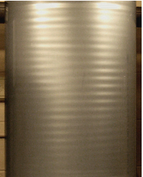
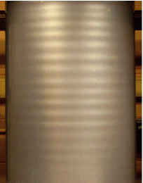
Figure 1: Elasto-rotational instability in visco-elastic Couette-Taylor flow. Left: Most unstable mode is $m=\pm 1$. Right: Most unstable mode is axisymmetric.

To argue that the observed instability is analogous to the magnetorotational instability, we performed another series of experiments. This time the gears at the cylinders were chosen to set up either quasi-Keplerian $\Omega(r)\propto r^{-1.3}$ or “anti-Keplerian” $\Omega(r)\propto r^{1.3}$ profiles. This is done to exclude the so-called elastic instability that can exist even for small Reynolds numbers (${\rm Re}=\Omega d^{2}/\eta_{P}$) as long as the Weissenberg number exceeds a certain threshold (Larson, Shaqfeh & Muller, 1990). The elastic instability takes energy from the elastic energy of the flow, and should not essentially depend on the sign of $\partial\Omega/\partial r$, while for the MRI the sign of $\partial\Omega/\partial r$ is crucial.

In the “anti-Keplerian” case, the only instability that could exist is purely elastic instability. For both considered concentrations of PolyOx, we observed the instability in the quasi-Keplerian case (analogous to the instability in the Keplerian case), however, we did not observed any instability in the anti-Keplerian case, even when we increased the shearing rates to three times as high as in the Keplerian counterpart. This indicates that in our Keplerian case the observed instability is driven by inertia and takes its energy from the kinetic energy of the flow. We therefore propose that the observed “elasto-rotational” instability is analogous to the magnetorotational instability.

Discussion.— Certain support for our observations is provided by the Ogilvie-Proctor consideration outlined in previous sections. We should be cautioned, however, that this model is to some extent phenomenological. It is known that the polymers fluid viscosity $\eta_{p}$ and relaxation time $\tau$ are not constants, but they strongly decrease as the shearing rate increases beyond $\dot{\gamma}\tau\simeq 1$ (the effect of shear-thinning). Besides, a model with single relaxation time is often not adequate, and one needs to introduce a series of relaxation times describing the relation between the shear rate and stress tensor. More essential, however, is the fact that in our case the polymer solution cannot be considered dilute for the used polymer concentrations. The application of the theory is therefore limited.

We however found that the theory is in reasonable agreement with the experiment if one substitutes the experimentally measured value for unknown viscosity $\eta_{p}$. Indeed, consider the case of the axisymmetric instability observed at polymer concentration $0.5\%$. We measured the shear viscosity of the flow $\eta_{p}$ at the obtained critical shearing rate $\dot{\gamma}_{c}$ by measuring the viscosity in a Bohlin rheometer using a system of two coaxial cylinders – a scaled down copy of the experimental set-up. The inner cylinder was stationary, and the outer cylinder rotated steadily so that the shear rate in the gap matched the shear rate in the experiment. The measured viscosity was $\eta_{p}(0.5)\approx 187{\rm mPa\cdot s}$. As for the relaxation time, it can be found for very low shearing rates using oscillation measurements, giving the value of order $\tau_{0}(0.5)\sim 1.4\,{\rm s}$. The relaxation time is however strongly shear-thinned at the experimental shear rate, so its precise value is difficult to evaluate.

We now substitute the experimental values of the critical shearing rate $\dot{\gamma}_{c}$, viscosity $\eta_{p}$, and the wave vector $k_{z}$, into the linearized Oldroid-B equations. Such linearized equations are derived in the limit of small but nonvanishing $d/R$ in (Larson, Shaqfeh & Muller, 1990); they are bulky and not presented here. We solved these equations numerically. The solution confirms that the axisymmetric instability with the observed parameters indeed exists if the fluid relaxation time is $\tau\sim 0.6{\rm s}$. This is a reasonable number if shear-thinning is taken into account. With this relaxation time we estimate that the instability occurs at ${\rm Wi}=\dot{\gamma}\tau\sim 4.4$ and ${\rm Re}=\dot{\gamma}d^{2}/\eta_{P}\sim 14$. Moreover, when we numerically switched to the anti-Keplerian profile by inverting the sign of the shearing rate $\dot{\gamma}$, the instability disappeared, which agrees with the experiment.

We note a useful fact that in the axisymmetric case ($m=0$), the instability threshold involves only $B_{3}=\sqrt{\eta_{p}/\tau}$. In the kinetic theory of dilute polymer solutions the ratio $\eta_{p}/\tau$ is constant and proportional only to polymer concentration (e.g., Doi & Edwards, 1986). Therefore the “imposed magnetic field” ${\bf B}_{3}$ is stable even when both polymer viscosity and relaxation time are shear-thinned by the flow. In the non-axisymmetric case ($m\neq 0$), the instability also depends on the azimuthal fields ${\bf B}_{1,2}$. In principle, it may be possible to design an experiment where such azimuthal field dominates, in even closer analogy with real accretion disks.

In conclusion, based on our results we propose that the analog of magnetorotational instability can be experimentally studied in visco-elastic flows of polymer fluids. For a more quantitative analysis and for direct comparison with the theory, different polymer solutions whose viscosities are not strongly shear-thinned should be used, the so-called Boger fluids (Boger, 1978). This work is in progress.