Trapped fermion mixtures with unequal masses: a Bogoliubov-de Gennes approach

Abstract

We use the Bogoliubov-de Gennes formalism to analyze the ground state phases of harmonically trapped two-species fermion mixtures with unequal masses. In the weakly attracting limit and around unitarity, we find that the superfluid order parameter is spatially modulated around the trap center, and that its global maximum occurs at a finite distance away from the trap center where the mixture is locally unpolarized. As the attraction strength increases towards the molecular limit, the spatial modulations gradually disappear while the Bardeen-Cooper-Schrieffer (BCS) type nonmodulated superfluid region expands until the entire mixture becomes locally unpolarized.

The many-body physics of fermion mixtures with mismatched Fermi surfaces has been a longstanding problem for many researchers ranging from the condensed and nuclear matter to the high energy and astrophysics communitites casalbuoni . While there are various theoretical proposals for the ground state of such systems including the Fulde-Ferrell-Larkin-Ovchinnikov (FFLO), Sarma and breached pair superfluid phases, strong experimental evidence for their observation is still lacking. Following the recent experiments on two-component ⁶Li mixtures with unequal populations mit ; rice , a new wave of theoretical interest in this problem has been sparked in the atomic and molecular physics communities. In these experiments the phase diagram of trapped (finite) systems has been studied as a function of population difference, temperature and two-body scattering length, showing superfluid and normal phases and a phase separation between them mit-pd .

Motivated by these experiments, phase diagrams of harmonically trapped mixtures with unequal populations have been extensively analyzed in both three- and one-dimensional systems. At the mean-field level in three dimensions, while fully quantum mechanical Bogoliubov-de Gennes (BdG) calculations provide some evidence for the FFLO type spatially modulated superfluid phase, such a phase is completely absent in calculations based on the semi-classical local density approximation (LDA) mizushima ; torma . Therefore, it is still an open question whether these spatial modulations are related to the FFLO superfluidity or are simply finite size effects. However, in exactly tractable one dimensional systems, FFLO structure of the superfluid phase have been identified in trapped as well as infinite systems 1Dorso ; 1Dhui ; feigun ; 1Dtezuka ; 1Dbatrouni . These works arguably suggest that the ground state of polarized mixtures is also an FFLO type superfluid in three dimensions along with the earlier BdG results mizushima ; torma .

Two-species fermion mixtures with unequal masses offer a very natural way of creating superfluidity with mismatched Fermi surfaces, and there have been increasing theoretical liu ; caldas ; iskin-mixture ; pao-mixture ; lin-mixture ; parish-mixture ; green ; orso-mixture ; baranov ; blume and experimental taglieber ; ville interest in studying such systems. For instance, ⁶Li-⁴⁰K mixtures have recently been trapped and interspecies Feshbach resonances have been identified taglieber ; ville , opening a new frontier in ultracold atom research to study exotic many-body phenomena. In this manuscript, we go beyond the LDA method pao-mixture ; lin-mixture , and use the BdG formalism to analyze the ground state phases of harmonically trapped ⁶Li-⁴⁰K mixtures. Our main results are as follows. In the weakly attracting limit and around unitarity, we find that the superfluid order parameter is spatially modulated around the trap center, and that its global maximum occurs at a finite distance away from the trap center where the mixture is locally unpolarized. As the attraction strength increases towards the molecular limit, the spatial modulations gradually disappear while the Bardeen-Cooper-Schrieffer (BCS) type nonmodulated superfluid region expands until the entire mixture becomes locally unpolarized as shown in Fig. 1.

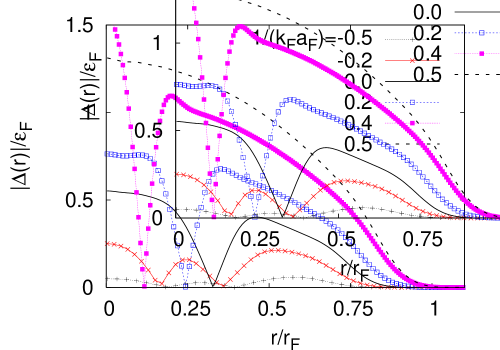
Figure 1: (Color online) The local superfluid order parameter $|\Delta(r)|$ versus distance $r$ is shown for a population balanced mixture of ⁶Li and ⁴⁰K atoms. The BCS type superfluidity first occurs at a finite distance away from the trap center where the mixture is locally unpolarized. As the attraction strength increases towards the molecular limit, it gradually expands until the entire mixture becomes locally unpolarized.

We obtain these results by using the following Hamiltonian (in units of $\hbar=k_{B}=1$)

$$H=\int d\mathbf{r}\left[\sum_{\sigma}\psi_{\sigma}^{\dagger}(\mathbf{r}){\cal K}_{\sigma}(\mathbf{r})\psi_{\sigma}(\mathbf{r})-g\Psi^{\dagger}(\mathbf{r})\Psi(\mathbf{r})\right],$$ (1)

to describe two-component fermion mixtures with zero-ranged attractive $(g>0)$ interactions, where $\psi_{\sigma}^{\dagger}(\mathbf{r})$ and $\psi_{\sigma}(\mathbf{r})$ field operators create and annihilate a pseudo-spin $\sigma$ fermion at position $\mathbf{r}$. Here, we have introduced the operators ${\cal K}_{\sigma}(\mathbf{r})=-\nabla^{2}/(2M_{\sigma})-\mu_{\sigma}(r)$ and $\Psi(\mathbf{r})=\psi_{\downarrow}(\mathbf{r})\psi_{\uparrow}(\mathbf{r}),$ where $M_{\sigma}$ is the mass, $\mu_{\sigma}(r)=\mu_{\sigma}-V_{\sigma}(r)$ is the local chemical potential, $\mu_{\sigma}$ is the global chemical potential and $V_{\sigma}(r)=M_{\sigma}\omega_{\sigma}^{2}r^{2}/2$ is the trapping potential of the $\sigma$ fermions. In the mean-field approximation for the superfluid phase, this Hamiltonian reduces to $H_{MF}=\int d\mathbf{r}[\sum_{\sigma}\psi_{\sigma}^{\dagger}(\mathbf{r}){\cal K}_{\sigma}(\mathbf{r})\psi_{\sigma}(\mathbf{r})-\Delta(\mathbf{r})\psi_{\uparrow}^{\dagger}(\mathbf{r})\psi_{\downarrow}^{\dagger}(\mathbf{r})-\Delta^{*}(\mathbf{r})\psi_{\downarrow}(\mathbf{r})\psi_{\uparrow}(\mathbf{r})+|\Delta(\mathbf{r})|^{2}/g],$ where the self-consistency field $\Delta(\mathbf{r})=g\langle\psi_{\uparrow}(\mathbf{r})\psi_{\downarrow}(\mathbf{r})\rangle$ is the local superfluid order parameter and $\langle...\rangle$ is a thermal average.

$H_{MF}$ can be diagonalized via the Bogoliubov-Valatin transformation $\psi_{\sigma}(\mathbf{r})=\sum_{\eta}[u_{\eta,\sigma}(\mathbf{r})\gamma_{\eta,\sigma}-s_{\sigma}v_{\eta,\sigma}^{*}(\mathbf{r})\gamma_{\eta,-\sigma}^{\dagger}],$ where $u_{\eta,\sigma}(\mathbf{r})$ and $v_{\eta,\sigma}(\mathbf{r})$ are the wavefunctions and $\gamma_{\eta,\sigma}^{\dagger}$ and $\gamma_{\eta,\sigma}$ are the operators corresponding to the creation and annihilation of a pseudo-spin $\sigma$ quasiparticle, and $s_{\uparrow}=+1$ and $s_{\downarrow}=-1$. This leads to the BdG equations

$$\left[\begin{array}[]{cc}{\cal K}_{\uparrow}(\mathbf{r})&\Delta(\mathbf{r})\\ \Delta^{*}(\mathbf{r})&-{\cal K}_{\downarrow}^{*}(\mathbf{r})\end{array}\right]\mathbf{\varphi_{\eta,\sigma}}(\mathbf{r})=s_{\sigma}\epsilon_{\eta,\sigma}\mathbf{\varphi_{\eta,\sigma}}(\mathbf{r}),$$ (2)

where $\epsilon_{\eta,\sigma}>0$ are the eigenvalues and $\mathbf{\varphi_{\eta,\sigma}}(\mathbf{r})$ are the eigenfunctions given by $\mathbf{\varphi_{\eta,\uparrow}}^{\dagger}(\mathbf{r})=[u_{\eta,\uparrow}^{*}(\mathbf{r}),v_{\eta,\downarrow}^{*}(\mathbf{r})]$ and $\mathbf{\varphi_{\eta,\downarrow}}^{\dagger}(\mathbf{r})=[v_{\eta,\uparrow}(\mathbf{r}),-u_{\eta,\downarrow}(\mathbf{r})].$ Since the BdG equations are invariant under the transformation $v_{\eta,\uparrow}(\mathbf{r})\to u_{\eta,\uparrow}^{*}(\mathbf{r})$, $u_{\eta,\downarrow}(\mathbf{r})\to-v_{\eta,\downarrow}^{*}(\mathbf{r})$ and $\epsilon_{\eta,\downarrow}\to-\epsilon_{\eta,\uparrow}$, it is sufficient to solve only for $u_{\eta}(\mathbf{r})\equiv u_{\eta,\uparrow}(\mathbf{r})$, $v_{\eta}(\mathbf{r})\equiv v_{\eta,\downarrow}(\mathbf{r})$ and $\epsilon_{\eta}\equiv\epsilon_{\eta,\uparrow}$ as long as we keep all of the solutions with positive and negative eigenvalues.

We assume $\Delta(\mathbf{r})=-g\sum_{\eta}u_{\eta}(\mathbf{r})v_{\eta}^{*}(\mathbf{r})f(\epsilon_{\eta})$ is real which is sufficient to describe both nonmodulated and spatially modulated superfluid phases. Here, $f(x)=1/[\exp(x/T)+1]$ is the Fermi function and $T$ is the temperature. This equation has an ultraviolet divergence due to zero-ranged interactions, and it can be regularized by relating $g$ to the two-body scattering length $a_{F}$ of the $\uparrow$ and $\downarrow$ fermions regularization . This leads to $1/g=-M_{r}/(4\pi a_{F})+M_{r}k_{c}(r)/(2\pi^{2})-[M_{r}k_{F}(r)/(4\pi^{2})]\log\{[k_{c}(r)+k_{F}(r)]/[k_{c}(r)-k_{F}(r)]\},$ where $M_{r}=2M_{\uparrow}M_{\downarrow}/(M_{\uparrow}+M_{\downarrow})$ is twice the reduced mass of the $\uparrow$ and $\downarrow$ fermions, $k_{F}^{2}(r)/(2M_{r})=[\mu_{\uparrow}(r)+\mu_{\downarrow}(r)]/2$ and $k_{c}^{2}(r)/(2M_{r})=\epsilon_{c}+[\mu_{\uparrow}(r)+\mu_{\downarrow}(r)]/2.$ Here, $\epsilon_{c}$ is the energy cutoff to be specified below, and our results depend weakly on the particular value of $\epsilon_{c}$ provided that it is chosen sufficiently high. Furthermore, the order parameter equation has to be solved self-consistently with the number equations $N_{\sigma}=\int d\mathbf{r}n_{\sigma}(\mathbf{r})$ where $n_{\sigma}(\mathbf{r})=\langle\psi_{\sigma}^{\dagger}(\mathbf{r})\psi_{\sigma}(\mathbf{r})\rangle$ is the local density of $\sigma$ fermions. This leads to $n_{\uparrow}(\mathbf{r})=\sum_{\eta}|u_{\eta}(\mathbf{r})|^{2}f(\epsilon_{\eta})$ and $n_{\downarrow}(\mathbf{r})=\sum_{\eta}|v_{\eta}(\mathbf{r})|^{2}f(-\epsilon_{\eta}).$

It is very natural to expand $u_{\eta}(\mathbf{r})$ and $v_{\eta}(\mathbf{r})$ in the complete basis of the harmonic trapping potential eigenfunctions, which are given by the Schrödinger’s equation ${\cal K}_{\sigma}(\mathbf{r})\phi_{n,\ell,m}^{\sigma}(\mathbf{r})=\xi_{n,\ell}^{\sigma}\phi_{n,\ell,m}^{\sigma}(\mathbf{r}),$ where $\xi_{n,\ell}^{\sigma}=\omega_{\sigma}(2n+\ell+3/2)-\mu_{\sigma}$ is the eigenvalue and $\phi_{n,\ell,m}^{\sigma}(\mathbf{r})=R_{n,\ell}^{\sigma}(r)Y_{\ell,m}(\theta_{\mathbf{r}},\varphi_{\mathbf{r}})$ is the eigenfunction. Here, $n$ is the radial quantum number, and $\ell$ and $m$ are the orbital angular momentum and its projection, respectively. The angular part $Y_{\ell,m}(\theta_{\mathbf{r}},\varphi_{\mathbf{r}})$ is a spherical harmonic and the radial part is $R_{n,\ell}^{\sigma}(r)=\sqrt{2}(M_{\sigma}\omega_{\sigma})^{3/4}[n!/(n+\ell+1/2)!]^{1/2}e^{-\bar{r}_{\sigma}^{2}/2}\bar{r}_{\sigma}^{\ell}L_{n}^{\ell+1/2}(\bar{r}_{\sigma}^{2}),$ where $\bar{r}_{\sigma}=\sqrt{M_{\sigma}\omega_{\sigma}}r$ is dimensionless and $L_{i}^{j}(x)$ is an associated Laguerre polynomial. Since $\ell$ and $m$ are good quantum numbers ($\eta\equiv\{\ell,m,\gamma\}$), this expansion leads to $u_{\ell,m,\gamma}(\mathbf{r})=\sum_{n}c_{\ell,\gamma,n}\phi_{n,\ell,m}^{\uparrow}(\mathbf{r})$ and $v_{\ell,m,\gamma}(\mathbf{r})=\sum_{n}d_{\ell,\gamma,n}\phi_{n,\ell,m}^{\downarrow}(\mathbf{r}).$

The spherical symmetry of the Hamiltonian simplifies the numerical calculations considerably such that the BdG equations reduce to a $2(n_{\ell}+1)\times 2(n_{\ell}+1)$ matrix eigenvalue problem for a given $\ell$ state

$$\sum_{n,n^{\prime}}\left(\begin{array}[]{cc}K_{\uparrow,\ell}^{n,n^{\prime}}&\Delta_{\ell}^{n,n^{\prime}}\\ \Delta_{\ell}^{n^{\prime},n}&-K_{\downarrow,\ell}^{n^{\prime},n}\end{array}\right)\left(\begin{array}[]{c}c_{\ell,\gamma,n^{\prime}}\\ d_{\ell,\gamma,n^{\prime}}\end{array}\right)=\epsilon_{\ell,\gamma}\sum_{n}\left(\begin{array}[]{c}c_{\ell,\gamma,n}\\ d_{\ell,\gamma,n}\end{array}\right),$$ (9)

where $n_{\ell}=(n_{c}-\ell)/2$ is the maximal radial quantum number and $n_{c}$ is the radial quantum number cutoff to be specified below. Here, the diagonal matrix element is $K_{\sigma,\ell}^{n,n^{\prime}}=\xi_{n,\ell}^{\sigma}\delta_{n,n^{\prime}}$ and the off-diagonal matrix element is $\Delta_{\ell}^{n,n^{\prime}}=\int r^{2}dr\Delta(r)R_{n,\ell}^{\uparrow}(r)R_{n^{\prime},\ell}^{\downarrow}(r),$ where $\delta_{i,j}$ is the Kronecker delta. Furthermore, this procedure reduces the order parameter equation to

$$\Delta(r)=-g\sum_{\ell,\gamma,n,n^{\prime}}\frac{2\ell+1}{4\pi}\widetilde{R}_{\ell,\gamma,n}^{\uparrow}(r)\widetilde{R}_{\ell,\gamma,n^{\prime}}^{\downarrow}(r)f(\epsilon_{\ell,\gamma}),$$ (10)

and the local density equations to

$$n_{\uparrow}(r) = \sum_{\ell,\gamma,n,n^{\prime}}\frac{2\ell+1}{4\pi}\widetilde{R}_{\ell,\gamma,n}^{\uparrow}(r)\widetilde{R}_{\ell,\gamma,n^{\prime}}^{\uparrow}(r)f(\epsilon_{\ell,\gamma}),$$ (11)

$$n_{\downarrow}(r) = \sum_{\ell,\gamma,n,n^{\prime}}\frac{2\ell+1}{4\pi}\widetilde{R}_{\ell,\gamma,n}^{\downarrow}(r)\widetilde{R}_{\ell,\gamma,n^{\prime}}^{\downarrow}(r)f(-\epsilon_{\ell,\gamma}),$$ (12)

where we introduced $\widetilde{R}_{\ell,\gamma,n}^{\uparrow}(r)=c_{\ell,\gamma,n}R_{n,\ell}^{\uparrow}(r)$ and $\widetilde{R}_{\ell,\gamma,n}^{\downarrow}(r)=d_{\ell,\gamma,n}R_{n,\ell}^{\downarrow}(r).$ Notice that the $(2\ell+1)$ factors in Eqs. (10), (11) and (12) are due to the degeneracy of each $\ell$ state. Furthermore, the total number equations become $N_{\uparrow}=\sum_{\ell,\gamma,n}(2\ell+1)c_{\ell,\gamma,n}^{2}f(\epsilon_{\ell,\gamma})$ and $N_{\downarrow}=\sum_{\ell,\gamma,n}(2\ell+1)d_{\ell,\gamma,n}^{2}f(-\epsilon_{\ell,\gamma}).$ These equations generalize the BdG formalism developed in Ref. ohashi to the case with unequal masses, unequal chemical potentials and/or unequal trapping potentials. Having discussed the BdG formalism, next we analyze the ground state ($T=0$) phases.

First, we analyze the noninteracting ($g=0$ or $a_{F}\to 0^{-}$) case. In this case, the discrete energy spectrum can be written as $\xi_{n,\ell}^{\sigma}=\omega_{\sigma}(n_{p}+3/2)$ where $n_{p}=2n+\ell$ is the principal quantum number. Therefore, for a given $n_{p}$, the orbital angular momentum $\ell$ ranges from $0,2,...,n_{p}$ when $n_{p}$ is even, and it ranges from $1,3,...,n_{p}$ when $n_{p}$ is odd. Since the single pseudo-spin degeneracy $D_{n_{p}}=\sum_{\ell}^{n_{p}}(2\ell+1)$ of each $n_{p}$ level is $D_{n_{p}}=(n_{p}+1)(n_{p}+2)/2,$ we can introduce the Fermi level $n_{F,\sigma}$ that corresponds to the maximal value of the occupied $n_{p}$ states at $T=0$. The condition $N_{\sigma}=\sum_{n_{p}=0}^{n_{F,\sigma}}D_{n_{p}}$ leads to $N_{\sigma}=(n_{F,\sigma}+1)(n_{F,\sigma}+2)(n_{F,\sigma}+3)/6,$ and the energy eigenvalue $\epsilon_{F,\sigma}=\omega_{\sigma}(n_{F,\sigma}+3/2)$ that corresponds to the $n_{p}=n_{F,\sigma}$ state is the Fermi energy of the $\sigma$ fermions. For sufficiently large $n_{F,\sigma}$, we notice that $\epsilon_{F,\sigma}$ and $N_{\sigma}$ have a simple relation $\epsilon_{F,\sigma}\approx\omega_{\sigma}(6N_{\sigma})^{1/3}$.

At $T=0$, we can approximately calculate the position $r_{*}$ where the local polarization density $p(r)=|n_{\uparrow}(r)-n_{\downarrow}(r)|$ becomes zero $p(r_{*})=0$. Using LDA, we find $n_{\sigma}(r)=k_{F,\sigma}^{3}(r)/(6\pi^{2}),$ where $k_{F,\sigma}(r)=M_{\sigma}\omega_{\sigma}(r_{F,\sigma}^{2}-r^{2})^{1/2}$ is the local Fermi momentum and $r_{F,\sigma}=(48N_{\sigma})^{1/6}/\sqrt{M_{\sigma}\omega_{\sigma}}$ is the Thomas-Fermi radius of the $\sigma$ fermions. This leads to $r_{*}=r_{F,\downarrow}[M_{\uparrow}\omega_{\uparrow}/(M_{\uparrow}\omega_{\uparrow}+M_{\downarrow}\omega_{\downarrow})]^{1/2},$ which is an important length scale because the formation of BCS type Cooper pairs is most favored in the momentum space regions when the Fermi surfaces of $\uparrow$ and $\downarrow$ fermions have minimal mismatch, i.e. $k_{F,\uparrow}(r_{*})=k_{F,\downarrow}(r_{*})$. Therefore, when $g\to 0^{+}$, the noninteracting mixture first becomes locally unstable against the BCS type superfluidity at $r_{*}$, as can be seen in our numerical calculations which is discussed next.

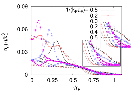
Figure 2: (Color online) The local density $n_{\sigma}(r)$ of ⁶Li (with points) and ⁴⁰K (with lines and points) atoms versus distance $r$ is shown for a population balanced mixture. The inset shows the close-up densities near the trap edge.

For this purpose, we solve the BdG equations 9, (10),  (11) and (12) self-consistently as a function of the dimensionless parameter $1/(k_{F}a_{F})$ where $k_{F}$ is specified below. In particular, we consider an equal population mixture of ⁶Li and ⁴⁰K atoms with $N_{\uparrow}=N_{\downarrow}$ and $M_{\uparrow}=0.15M_{\downarrow}$, and assume that both ⁶Li and ⁴⁰K atoms are trapped with equal trapping potentials $V_{\uparrow}(r)=V_{\downarrow}(r)$ such that $M_{\uparrow}\omega_{\uparrow}^{2}=M_{\downarrow}\omega_{\downarrow}^{2}$. We introduce a ‘reduced’ trapping frequency $\omega_{r}$ via $M_{r}\omega_{r}^{2}=M_{\sigma}\omega_{\sigma}^{2}$, and define an energy scale $\epsilon_{F}$ and two length scales $(k_{F},r_{F})$ via $\epsilon_{F}=\omega_{r}(n_{F}+3/2)=k_{F}^{2}/(2M_{r})=M_{r}\omega_{r}^{2}r_{F}^{2}/2.$ Notice that $n_{F}=n_{F,\uparrow}=n_{F,\downarrow}$ when $N_{\uparrow}=N_{\downarrow}$. Similarly, we define $n_{c}$ via $\epsilon_{c}=\omega_{r}(n_{c}+3/2)$. In our numerical calculations, we choose $n_{F}=15$ and $n_{c}=65$, which correspond to a total of $N=1632$ fermions and $\epsilon_{c}\approx 4\epsilon_{F}$, respectively. Here, it is important to emphasize that we do not expect any qualitative change in our results with higher values of $n_{F}$ and/or $n_{c}$, except for minor quantitative variations.

In Figs. 1, 2 and 3, we show the evolution of $\Delta(r)$, $n_{\sigma}(r)$ and $p(r)$ as a function of $1/(k_{F}a_{F})$. For a weakly attracting mixture, while ⁴⁰K atoms are in excess around the trap center and ⁶Li atoms are in excess close to the trap edge, they have similar densities only around $r=r_{*}\approx 0.85r_{F,\downarrow}\approx 0.61r_{F}$. Therefore, when $1/(k_{F}a_{F})\lesssim-0.5$, we find that $\Delta(r)$ is spatially modulated around $r=0$, and that its global maximum occurs at $r=r_{*}$ where the mixture is locally unpolarized. The modulation period ${\cal T}\approx 0.6r_{F}$ of $\Delta(r)$ is approximately given by ${\cal T}\sim 2\pi/|k_{F,\uparrow}-k_{F,\downarrow}|\approx 0.5r_{F}$, where $k_{F,\sigma}=\sqrt{2M_{\sigma}\mu_{\sigma}}$. As $g$ increases towards unitarity $1/(k_{F}a_{F})=0$, we find that the amplitude of the modulations dramatically increases around $r=0$. This is because both $n_{\uparrow}(r)$ and $n_{\downarrow}(r)$ are highest at $r=0$, which effectively leads to stronger local interactions there since $1/[k_{F}(r)a_{F}]$ increases with increasing density when $a_{F}<0$. Therefore, the maximum of $\Delta(r)$ eventually occurs at $r=0$ when the effective local interactions become sufficiently strong.

These spatial modulations of $\Delta(r)$ have dramatic effects on the local density of fermions causing pronounced modulations in $n_{\sigma}(r)$ and $p(r)$ close to $r=0$ as shown in Figs. 2 and 3. Since these modulations are significantly large, we hope that they can be observed in the future experiments. Further increasing $g$ towards the molecular limit $1/(k_{F}a_{F})\gtrsim 0.5$, we find that the spatial modulations gradually disappear and the BCS type nonmodulated superfluid region expands until the entire mixture becomes locally unpolarized. This is expected because the Fermi surfaces disappear in this limit, and therefore formation of the molecules does not require matching of the Fermi surfaces.

We remark in passing that the BdG equations do not necessarily have a unique solution, and depending on the initial values of $\mu_{\sigma}$ and $\Delta(r)$ that are used in the iterative approach, they often yield multiple solutions for a given set of parameters. In this manuscript, we show only the physical solutions which have lowest energy. Compared to the physical solutions, the unphysical ones have considerable qualitative variations around $r=0$, i.e. both $\Delta(r)$ and $n_{\sigma}(r)$ have more modulations. However, both the physical and the unphysical solutions have very similar qualitative structure around $r=r_{*}$, where the BCS type nonmodulated superfluidity occurs.

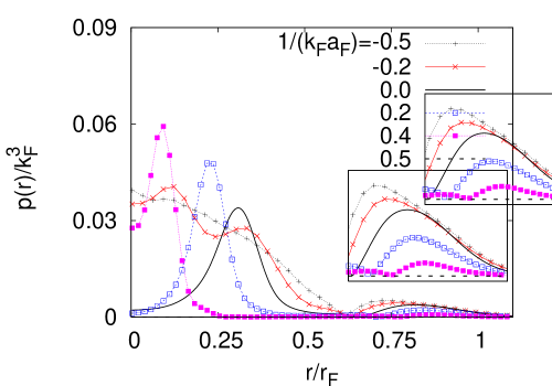
Figure 3: (Color online) The local polarization density $p(r)=|n_{\uparrow}(r)-n_{\downarrow}(r)|$ versus distance $r$ is shown for a population balanced mixture of ⁶Li and ⁴⁰K atoms. While ⁶Li atoms are in excess near the trap edge, ⁴⁰K atoms are in excess close to the center.

We emphasize that our results are based on the fully quantum mechanical BdG formalism, and that they are significantly different from the earlier results that are based on the semi-classical LDA method pao-mixture ; lin-mixture . For instance, these LDA calculations suggest a sharp phase separation in the weakly attracting limit and around unitarity such that the BCS type superfluid phase is sandwiched between locally polarized normal fermions. Therefore, both $\Delta(r)$ and $n_{\sigma}(r)$ have unphysical discontinuities at the normal-BCS superfluid-normal interfaces which indicates breakdown of the LDA. This is because the LDA method excludes the possibility of a spatially modulated superfluid phase, which is one of the possible candidates for the ground state. A similar discrepancy between the BdG and the LDA method was previously discussed in the context of one-species fermion mixtures with unequal populations mizushima ; torma . Thus, we conclude quite generally that the LDA method is insufficient to describe trapped fermion mixtures with mismatched Fermi surfaces, and that it should be used with caution.

Furthermore, our results for population balanced two-species fermion mixtures are qualitatively different from the recent works on one-species fermion mixtures with unequal populations mizushima ; torma . In the latter case, the BCS type superfluid phase occurs around $r=0$, and $\Delta(r)$ is spatially modulated towards the trap edge where the mixture is locally polarized. Since both $n_{\uparrow}(r)$ and $n_{\downarrow}(r)$ are very low near the trap edge and the modulations have very small amplitudes, it may not be possible to observe them at experimentally attainable temperatures. However, in our case, spatial modulations with large amplitudes occur around $r=0$ where both $n_{\uparrow}(r)$ and $n_{\downarrow}(r)$ are very high. These make two-species fermion mixtures very good candidates for the observation of spatially modulated superfluid phases in atomic systems.

For instance, spatial modulations of $\Delta(r)$ can be observed by using the recently developed technique of spatially resolved radio-frequency spectroscopy shin-rf . This technique can be used to locate the nodes of $\Delta(r)$, since the local quasiparticle excitation spectrum becomes gapless at the position of the nodes. In addition, spatial modulations of $n_{\sigma}(r)$ can be observed by using phase-contrast imaging of ⁶Li and ⁴⁰K populations. In fact, both of these techniques have recently been used with great success to characterize the superfluid and the normal phases of one-species fermion mixtures with unequal populations shin-rf .

In conclusion, we analyzed the ground state phases of harmonically trapped ⁶Li-⁴⁰K mixtures with equal populations. In the weakly interacting limit and around unitarity, we found that the superfluid order parameter is spatially modulated around the trap center. Furthermore, we showed that the BCS type superfluidity first occurs at a finite distance away from the trap center where the mixture is locally unpolarized, and then it gradually expands as the attraction strength increases towards the molecular limit until the entire mixture becomes locally unpolarized. Since the spatial modulations with large amplitudes survive at unitarity, two-species fermion mixtures offer a unique opportunity for their observation.

References

(1) R. Casalbuoni and G. Nardulli, Rev. Mod. Phys. 76, 263 (2004).
(2) M. W. Zwierlein et al., Science 311, 492 (2006).
(3) G. B. Partridge et al., Science 311, 503 (2006).
(4) Y. Shin et al., Nature 451, 689 (2008).
(5) T. Mizushima et al., J. Phys. Soc. Jpn. 76, 104006 (2007).
(6) L. M. Jensen, J. Kinnunen, and P. Törmä, Phys. Rev. A 76, 033620 (2007).
(7) G. Orso, Phys. Rev. Lett. 98, 070402 (2007).
(8) Hui Hu, Xia-Ji Liu, and Peter D. Drummond, Phys. Rev. Lett. 98, 070403 (2007).
(9) A. E. Feiguin and F. Heidrich-Meisner, Phys. Rev. B 76, 220508(R) (2007).
(10) M. Tezuka and M. Ueda, Phys. Rev. Lett. 100, 110403 (2008).
(11) G. G. Batrouni et al., Phys. Rev. Lett. 100, 116405 (2008).
(12) W.V. Liu and F. Wilczek, Phys. Rev. Lett. 90, 047002 (2003).
(13) P. F. Bedaque, H. Caldas, and G. Rupak, Phys. Rev. Lett. 91, 247002 (2003).
(14) M. Iskin and C. A. R. Sá de Melo, Phys. Rev. Lett. 97, 100404 (2006);
Phys. Rev. A 76, 013601 (2007); Phys. Rev. A 77, 013625 (2008).
(15) C.-H. Pao, Shin-Tza Wu, and S.-K. Yip, Phys. Rev. B 74, 224504 (2006);
Phys. Rev. A 76, 053621 (2007).
(16) G.-D. Lin, W. Yi, and L.-M. Duan, Phys. Rev. A 74, 031604(R) (2006).
(17) M. M. Parish et al., Phys. Rev. Lett. 98, 160402 (2007).
(18) J. von Stecher, C. H. Greene, and D. Blume, Phys. Rev. A 76, 053613 (2007).
(19) G. Orso, L. P. Pitaevskii, and S. Stringari, Phys. Rev. A 77, 033611 (2008).
(20) M.A. Baranov, C. Lobo, and G. V. Shlyapnikov, Phys. Rev. A 78, 033620 (2008).
(21) D. Blume, Phys. Rev. A 78, 013613 (2008).
(22) M. Taglieber et al., Phys. Rev. Lett. 100, 010401 (2008).
(23) E. Wille et al., Phys. Rev. Lett. 100, 053201 (2008).
(24) A. Bulgac and Y. Yu, Phys. Rev. Lett. 88, 042504 (2002).
(25) Y. Ohashi and A. Griffin, Phys. Rev. A 72, 013601 (2005).
(26) Y. Shin et al., Phys. Rev. Lett. 99, 090403 (2007).