Abstract

Three-wave interactions ($\mbox{M}\leftrightarrow\mbox{P}+\mbox{Q}$) of plasma waves propagating parallel to the mean magnetic field at frequencies below the electron cyclotron frequency are considered. We consider Alfvén–ion-cyclotron waves (L), fast-magnetosonic–whistler waves (R), and ion-sound waves (I). Especially the weakly turbulent low-beta plasmas like the solar corona are studied, using the cold-plasma dispersion relation for the transverse waves (L, R) and the fluid-description of the warm plasma for the longitudinal waves (I). We analyse the resonance conditions for the wave frequencies $\omega$ and wavenumbers $k$ (i.e., $\omega_{\rm M}=\omega_{\rm P}+\omega_{\rm Q}$ and $k_{\rm M}=k_{\rm P}\pm k_{\rm Q}$, and the interaction rates $u^{\rm MPQ}$ of the waves for all possible combinations of the three wave modes, and list those reactions that are not forbidden. One of the waves has to be longitudinal and two transverse. This demonstrates an attractive feature of the theory: the conservation of angular momentum is implicitly built in. In a low-beta plasma, non-zero reaction rates are obtained for (i) $\mbox{L}^{+}\leftrightarrow\mbox{I}^{+}+\mbox{L}^{-}$ and $\mbox{R}^{+}\leftrightarrow\mbox{I}^{+}+\mbox{R}^{-}$ in a wide frequency range extending from the MHD frequency range to the resonances of the waves; (ii) for $\mbox{L}^{+}\leftrightarrow\mbox{L}^{+}+\mbox{I}^{+}$ in more narrow frequency range, where at least one of the L waves is in the dispersive frequency range; and (iii) $\mbox{I}^{+}\leftrightarrow\mbox{L}^{+}+\mbox{R}^{\pm}$ close to the resonance of the L mode. The reaction types (ii) and (iii) have, to our knowledge, not been discussed before in low-beta plasmas. In high-beta plasmas, reactions $\mbox{I}^{+}\leftrightarrow\mbox{R}^{+}+\mbox{L}^{-}$ and $\mbox{I}^{+}\leftrightarrow\mbox{L}^{+}+\mbox{R}^{-}$ are the main reactions, extending down to the MHD frequencies and discussed earlier for the non-dispersive case, but new reactions involving dispersive waves are found in high-beta plasmas as well: $\mbox{I}^{+}\leftrightarrow\mbox{L}^{+}+\mbox{R}^{+}$ and $\mbox{R}^{+}\leftrightarrow\mbox{I}^{+}+\mbox{R}^{\pm}$ are now possible in limited frequency ranges involving at least one dispersive transverse wave. We discuss the implications of the discovered new reactions to turbulent cascading in space plasmas.
Keywords: plasma waves – turbulence – wave-wave interactions

1 Introduction

Three-wave interactions constitute the lowest-order non-linear coupling between wave-modes in plasmas. These interactions are of form, where either two modes coalesce into one or one mode decays into two, i.e., $\mbox{M}\leftrightarrow\mbox{P}+\mbox{Q}$, with momentum and energy being conserved at microscopic level, i.e., $\omega_{{\rm M}}=\omega_{{\rm P}}+\omega_{{\rm Q}}$ and $\mathchoice{\mbox{\boldmath$\displaystyle k$}}{\mbox{\boldmath$\textstyle k$}}{\mbox{\boldmath$\scriptstyle k$}}{\mbox{\boldmath$\scriptscriptstyle k$}}_{{\rm M}}=\mathchoice{\mbox{\boldmath$\displaystyle k$}}{\mbox{\boldmath$\textstyle k$}}{\mbox{\boldmath$\scriptstyle k$}}{\mbox{\boldmath$\scriptscriptstyle k$}}_{{\rm P}}+\mathchoice{\mbox{\boldmath$\displaystyle k$}}{\mbox{\boldmath$\textstyle k$}}{\mbox{\boldmath$\scriptstyle k$}}{\mbox{\boldmath$\scriptscriptstyle k$}}_{{\rm Q}}$. Thus, three-wave interactions provide the leading-order description of the evolution of weak turbulence, where it is assumed that the amplitudes of the interacting wave packets are small enough for a perturbation theory approach to apply. Turbulence evolution, on the other hand, is one of the key issues in plasma astrophysics and space physics. It is intimately related to fundamental questions like plasma heating and particle acceleration and transport in collisionless plasmas. To get started with weak turbulence theory, the reader is referred to [1].

In this paper we will investigate three-wave interactions of plasma waves propagating parallel to the mean magnetic field in a magnetised, low-beta plasma. The pioneering work by Chin and Wentzel [2] considered three-wave interactions between low-frequency plasma waves under the random-phase approximation, assuming that the waves fulfill the MHD dispersion relations, i.e., $\omega=v_{{\rm A}}k_{\parallel}$ for the transverse waves and $\omega=v_{{\rm S}}k_{\parallel}$ for the longitudinal waves. Their study revealed that for a low-beta plasma, three-wave interactions where an Alfvén wave decays into a parallel-propagating sound wave and an anti-parallel-propagating Alfvén wave, i.e., $\mbox{A}^{+}\leftrightarrow\mbox{S}^{+}+\mbox{A}^{-}$, dominate the evolution of weak turbulence. In these interactions, the number of Alfvén wave quanta is conserved, and since the sound waves are generally easily damped, the interactions proceed typically in the direction of wave decay. Thus, their study predicted an inverse cascade of energy from high to low frequencies with a simultaneous heating of the plasma by the dissipation of the sound waves emitted by the three-wave interaction. Their model has been applied by numerous authors to study different astrophysical scenarios from the heating of the solar corona [3] to the confinement and transport of cosmic rays (CR) in the galaxy [4] and more recently to CR acceleration in astrophysical shocks [5]. The work of Chin and Wentzel, however, was developed under the MHD approximation. In this work, we will consider an extension to the work by adopting dispersion relations more suitable for a collisionless plasma [1, 6]. Specifically, we will consider interactions between left- and right-hand circularly polarised transverse waves and longitudinal ion sound waves at frequencies well below the electron gyro-frequency. We will apply the results of the analysis to conditions in the solar corona, pointing out several new evolution scenarios of parallel propagating plasma waves, which have relevance to, e.g., coronal heating and particle acceleration at the Sun. This treatment is considered a kinetic treatment for two major reasons: First of all we are not using the limited MHD dispersion relations which would not hold for frequencies well above the ion gyrofrequency. Secondly we are not bound to thermal distribution functions of the background plasma, which means we do not depend on collisions to produce thermal distributions. As will be shown later in this paper for Maxwellian distributions, however, the actual interactions only depend on the parameter $\beta$ and the ratio $\Omega_{\textrm{i}}/\omega_{\textrm{pi}}$.

The structure of the paper is as follows: in §2 we will summarise the theory of three-wave interactions for collisionless plasmas, in §3 we will analyse in detail the three-wave interactions between plasma waves propagating parallel to the magnetic field, in §4 we will discuss the results and present the conclusions from the analysis.

2 Three-wave interactions in a collisionless plasma

The framework used here to describe the interaction of waves in collisionless plasmas employs a quasi-particle description of waves derived previously by [2] and described in detail by [1] and references therein. These theories are, as already mentioned above, usually derived for a fluid plasma (for [2]) or an unmagnetised plasma (as in [1]).

Our calculations in the kinetic limit for magnetised plasmas follow [7] using the interaction tensor from [8]. The physical picture is the following: The interaction of waves is transmitted by the electric field of these waves. From this interaction an infinite series of interaction terms is given, where the linear (first order) term describes the propagation and the first nonlinear (quadratic) term is the simplest form of interaction.

Given three reservoirs of wave quanta denoted by $N^{\mathrm{M}}$, $N^{\mathrm{P}}$, and $N^{\mathrm{Q}}$ the evolution equation for the occupation number of the wave quanta is given by

$$\frac{\partial N^{\mathrm{M}}(\mathchoice{\mbox{\boldmath$\displaystyle k$}}{\mbox{\boldmath$\textstyle k$}}{\mbox{\boldmath$\scriptstyle k$}}{\mbox{\boldmath$\scriptscriptstyle k$}})}{\partial t} = \int\frac{\mathrm{d}^{3}k^{\prime}}{(2\pi)^{3}}\int\frac{\mathrm{d}^{3}k^{\prime\prime}}{(2\pi)^{3}}u^{\mathrm{MPQ}}(\mathchoice{\mbox{\boldmath$\displaystyle k$}}{\mbox{\boldmath$\textstyle k$}}{\mbox{\boldmath$\scriptstyle k$}}{\mbox{\boldmath$\scriptscriptstyle k$}},\mathchoice{\mbox{\boldmath$\displaystyle k$}}{\mbox{\boldmath$\textstyle k$}}{\mbox{\boldmath$\scriptstyle k$}}{\mbox{\boldmath$\scriptscriptstyle k$}}^{\prime},\mathchoice{\mbox{\boldmath$\displaystyle k$}}{\mbox{\boldmath$\textstyle k$}}{\mbox{\boldmath$\scriptstyle k$}}{\mbox{\boldmath$\scriptscriptstyle k$}}^{\prime\prime})$$ (1)

$$\times\left\{N^{\mathrm{P}}(\mathchoice{\mbox{\boldmath$\displaystyle k$}}{\mbox{\boldmath$\textstyle k$}}{\mbox{\boldmath$\scriptstyle k$}}{\mbox{\boldmath$\scriptscriptstyle k$}}^{\prime})N^{\mathrm{Q}}(\mathchoice{\mbox{\boldmath$\displaystyle k$}}{\mbox{\boldmath$\textstyle k$}}{\mbox{\boldmath$\scriptstyle k$}}{\mbox{\boldmath$\scriptscriptstyle k$}}^{\prime\prime})-N^{\mathrm{M}}(\mathchoice{\mbox{\boldmath$\displaystyle k$}}{\mbox{\boldmath$\textstyle k$}}{\mbox{\boldmath$\scriptstyle k$}}{\mbox{\boldmath$\scriptscriptstyle k$}})[N^{\mathrm{P}}(\mathchoice{\mbox{\boldmath$\displaystyle k$}}{\mbox{\boldmath$\textstyle k$}}{\mbox{\boldmath$\scriptstyle k$}}{\mbox{\boldmath$\scriptscriptstyle k$}}^{\prime})+N^{\mathrm{Q}}(\mathchoice{\mbox{\boldmath$\displaystyle k$}}{\mbox{\boldmath$\textstyle k$}}{\mbox{\boldmath$\scriptstyle k$}}{\mbox{\boldmath$\scriptscriptstyle k$}}^{\prime\prime})]\right\}$$

$$\frac{\partial N^{\mathrm{P}}(\mathchoice{\mbox{\boldmath$\displaystyle k$}}{\mbox{\boldmath$\textstyle k$}}{\mbox{\boldmath$\scriptstyle k$}}{\mbox{\boldmath$\scriptscriptstyle k$}}^{\prime})}{\partial t} = -\int\frac{\mathrm{d}^{3}k}{(2\pi)^{3}}\int\frac{\mathrm{d}^{3}k^{\prime\prime}}{(2\pi)^{3}}u^{\mathrm{MPQ}}(\mathchoice{\mbox{\boldmath$\displaystyle k$}}{\mbox{\boldmath$\textstyle k$}}{\mbox{\boldmath$\scriptstyle k$}}{\mbox{\boldmath$\scriptscriptstyle k$}},\mathchoice{\mbox{\boldmath$\displaystyle k$}}{\mbox{\boldmath$\textstyle k$}}{\mbox{\boldmath$\scriptstyle k$}}{\mbox{\boldmath$\scriptscriptstyle k$}}^{\prime},\mathchoice{\mbox{\boldmath$\displaystyle k$}}{\mbox{\boldmath$\textstyle k$}}{\mbox{\boldmath$\scriptstyle k$}}{\mbox{\boldmath$\scriptscriptstyle k$}}^{\prime\prime})$$ (2)

$$\times\left\{N^{\mathrm{P}}(\mathchoice{\mbox{\boldmath$\displaystyle k$}}{\mbox{\boldmath$\textstyle k$}}{\mbox{\boldmath$\scriptstyle k$}}{\mbox{\boldmath$\scriptscriptstyle k$}}^{\prime})N^{\mathrm{Q}}(\mathchoice{\mbox{\boldmath$\displaystyle k$}}{\mbox{\boldmath$\textstyle k$}}{\mbox{\boldmath$\scriptstyle k$}}{\mbox{\boldmath$\scriptscriptstyle k$}}^{\prime\prime})-N^{\mathrm{M}}(\mathchoice{\mbox{\boldmath$\displaystyle k$}}{\mbox{\boldmath$\textstyle k$}}{\mbox{\boldmath$\scriptstyle k$}}{\mbox{\boldmath$\scriptscriptstyle k$}})[N^{\mathrm{P}}(\mathchoice{\mbox{\boldmath$\displaystyle k$}}{\mbox{\boldmath$\textstyle k$}}{\mbox{\boldmath$\scriptstyle k$}}{\mbox{\boldmath$\scriptscriptstyle k$}}^{\prime})+N^{\mathrm{Q}}(\mathchoice{\mbox{\boldmath$\displaystyle k$}}{\mbox{\boldmath$\textstyle k$}}{\mbox{\boldmath$\scriptstyle k$}}{\mbox{\boldmath$\scriptscriptstyle k$}}^{\prime\prime})]\right\}$$

$$\frac{\partial N^{\mathrm{Q}}(\mathchoice{\mbox{\boldmath$\displaystyle k$}}{\mbox{\boldmath$\textstyle k$}}{\mbox{\boldmath$\scriptstyle k$}}{\mbox{\boldmath$\scriptscriptstyle k$}}^{\prime\prime})}{\partial t} = -\int\frac{\mathrm{d}^{3}k}{(2\pi)^{3}}\int\frac{\mathrm{d}^{3}k^{\prime}}{(2\pi)^{3}}u^{\mathrm{MPQ}}(\mathchoice{\mbox{\boldmath$\displaystyle k$}}{\mbox{\boldmath$\textstyle k$}}{\mbox{\boldmath$\scriptstyle k$}}{\mbox{\boldmath$\scriptscriptstyle k$}},\mathchoice{\mbox{\boldmath$\displaystyle k$}}{\mbox{\boldmath$\textstyle k$}}{\mbox{\boldmath$\scriptstyle k$}}{\mbox{\boldmath$\scriptscriptstyle k$}}^{\prime},\mathchoice{\mbox{\boldmath$\displaystyle k$}}{\mbox{\boldmath$\textstyle k$}}{\mbox{\boldmath$\scriptstyle k$}}{\mbox{\boldmath$\scriptscriptstyle k$}}^{\prime\prime})$$ (3)

$$\times\left\{N^{\mathrm{P}}(\mathchoice{\mbox{\boldmath$\displaystyle k$}}{\mbox{\boldmath$\textstyle k$}}{\mbox{\boldmath$\scriptstyle k$}}{\mbox{\boldmath$\scriptscriptstyle k$}}^{\prime})N^{\mathrm{Q}}(\mathchoice{\mbox{\boldmath$\displaystyle k$}}{\mbox{\boldmath$\textstyle k$}}{\mbox{\boldmath$\scriptstyle k$}}{\mbox{\boldmath$\scriptscriptstyle k$}}^{\prime\prime})-N^{\mathrm{M}}(\mathchoice{\mbox{\boldmath$\displaystyle k$}}{\mbox{\boldmath$\textstyle k$}}{\mbox{\boldmath$\scriptstyle k$}}{\mbox{\boldmath$\scriptscriptstyle k$}})[N^{\mathrm{P}}(\mathchoice{\mbox{\boldmath$\displaystyle k$}}{\mbox{\boldmath$\textstyle k$}}{\mbox{\boldmath$\scriptstyle k$}}{\mbox{\boldmath$\scriptscriptstyle k$}}^{\prime})+N^{\mathrm{Q}}(\mathchoice{\mbox{\boldmath$\displaystyle k$}}{\mbox{\boldmath$\textstyle k$}}{\mbox{\boldmath$\scriptstyle k$}}{\mbox{\boldmath$\scriptscriptstyle k$}}^{\prime\prime})]\right\}.$$

Here, the primed [double-primed] quantities refer to the mode P[Q] and the unprimed quantities to mode M. The interaction rate is defined as

$$u^{\mathrm{MPQ}}(\mathchoice{\mbox{\boldmath$\displaystyle k$}}{\mbox{\boldmath$\textstyle k$}}{\mbox{\boldmath$\scriptstyle k$}}{\mbox{\boldmath$\scriptscriptstyle k$}},\mathchoice{\mbox{\boldmath$\displaystyle k$}}{\mbox{\boldmath$\textstyle k$}}{\mbox{\boldmath$\scriptstyle k$}}{\mbox{\boldmath$\scriptscriptstyle k$}}^{\prime},\mathchoice{\mbox{\boldmath$\displaystyle k$}}{\mbox{\boldmath$\textstyle k$}}{\mbox{\boldmath$\scriptstyle k$}}{\mbox{\boldmath$\scriptscriptstyle k$}}^{\prime\prime}) = \frac{8(2\pi)^{7}\hbar c^{4}}{\omega^{\mathrm{M}}\omega^{\mathrm{P}}\omega^{\mathrm{Q}}}\frac{W_{E}^{\mathrm{M}}}{W_{\mathrm{T}}^{\mathrm{M}}}\frac{W_{E}^{\mathrm{P}}}{W_{\mathrm{T}}^{\mathrm{P}}}\frac{W_{E}^{\mathrm{Q}}}{W_{\mathrm{T}}^{\mathrm{Q}}}\times$$ (4)

$$|\kappa^{\mathrm{MPQ}}(\mathchoice{\mbox{\boldmath$\displaystyle k$}}{\mbox{\boldmath$\textstyle k$}}{\mbox{\boldmath$\scriptstyle k$}}{\mbox{\boldmath$\scriptscriptstyle k$}},\mathchoice{\mbox{\boldmath$\displaystyle k$}}{\mbox{\boldmath$\textstyle k$}}{\mbox{\boldmath$\scriptstyle k$}}{\mbox{\boldmath$\scriptscriptstyle k$}}^{\prime},\mathchoice{\mbox{\boldmath$\displaystyle k$}}{\mbox{\boldmath$\textstyle k$}}{\mbox{\boldmath$\scriptstyle k$}}{\mbox{\boldmath$\scriptscriptstyle k$}}^{\prime\prime})|^{2}\delta^{3}(\mathchoice{\mbox{\boldmath$\displaystyle k$}}{\mbox{\boldmath$\textstyle k$}}{\mbox{\boldmath$\scriptstyle k$}}{\mbox{\boldmath$\scriptscriptstyle k$}}-\mathchoice{\mbox{\boldmath$\displaystyle k$}}{\mbox{\boldmath$\textstyle k$}}{\mbox{\boldmath$\scriptstyle k$}}{\mbox{\boldmath$\scriptscriptstyle k$}}^{\prime}-\mathchoice{\mbox{\boldmath$\displaystyle k$}}{\mbox{\boldmath$\textstyle k$}}{\mbox{\boldmath$\scriptstyle k$}}{\mbox{\boldmath$\scriptscriptstyle k$}}^{\prime\prime})\delta(\omega-\omega^{\prime}-\omega^{\prime\prime})$$

The interaction can be derived when using the vector potential of the electric field (in temporal gauge). From the vector potential of all involved waves the response tensor can be calculated, which is basically given by the quantity $u^{\mathrm{MPQ}}$. In weak turbulence theory the response tensor is calculated only to the second order in the vector potentials. The fact that the electric fields are interacting is resembled by the factor $W_{E}/W_{\mathrm{T}}$, which simply describes the ratio of electric to total energy. The physical details of the response tensor are now hidden in $\kappa^{\mathrm{MPQ}}$:

$$\kappa^{\mathrm{MPQ}}(\mathchoice{\mbox{\boldmath$\displaystyle k$}}{\mbox{\boldmath$\textstyle k$}}{\mbox{\boldmath$\scriptstyle k$}}{\mbox{\boldmath$\scriptscriptstyle k$}},\mathchoice{\mbox{\boldmath$\displaystyle k$}}{\mbox{\boldmath$\textstyle k$}}{\mbox{\boldmath$\scriptstyle k$}}{\mbox{\boldmath$\scriptscriptstyle k$}}^{\prime},\mathchoice{\mbox{\boldmath$\displaystyle k$}}{\mbox{\boldmath$\textstyle k$}}{\mbox{\boldmath$\scriptstyle k$}}{\mbox{\boldmath$\scriptscriptstyle k$}}^{\prime\prime}) = (e_{i}^{\mathrm{M}})^{*}e_{j}^{\mathrm{P}}e_{l}^{\mathrm{Q}}\kappa_{ijl}(\mathchoice{\mbox{\boldmath$\displaystyle k$}}{\mbox{\boldmath$\textstyle k$}}{\mbox{\boldmath$\scriptstyle k$}}{\mbox{\boldmath$\scriptscriptstyle k$}},\omega;\mathchoice{\mbox{\boldmath$\displaystyle k$}}{\mbox{\boldmath$\textstyle k$}}{\mbox{\boldmath$\scriptstyle k$}}{\mbox{\boldmath$\scriptscriptstyle k$}}^{\prime},\omega^{\prime};\mathchoice{\mbox{\boldmath$\displaystyle k$}}{\mbox{\boldmath$\textstyle k$}}{\mbox{\boldmath$\scriptstyle k$}}{\mbox{\boldmath$\scriptscriptstyle k$}}^{\prime\prime},\omega^{\prime\prime})$$ (5)

$$\kappa_{ijl}(\mathchoice{\mbox{\boldmath$\displaystyle k$}}{\mbox{\boldmath$\textstyle k$}}{\mbox{\boldmath$\scriptstyle k$}}{\mbox{\boldmath$\scriptscriptstyle k$}},\mathchoice{\mbox{\boldmath$\displaystyle k$}}{\mbox{\boldmath$\textstyle k$}}{\mbox{\boldmath$\scriptstyle k$}}{\mbox{\boldmath$\scriptscriptstyle k$}}^{\prime},\mathchoice{\mbox{\boldmath$\displaystyle k$}}{\mbox{\boldmath$\textstyle k$}}{\mbox{\boldmath$\scriptstyle k$}}{\mbox{\boldmath$\scriptscriptstyle k$}}^{\prime\prime}) = \frac{1}{2}\left[\tilde{\kappa}_{ijl}(\mathchoice{\mbox{\boldmath$\displaystyle k$}}{\mbox{\boldmath$\textstyle k$}}{\mbox{\boldmath$\scriptstyle k$}}{\mbox{\boldmath$\scriptscriptstyle k$}},\mathchoice{\mbox{\boldmath$\displaystyle k$}}{\mbox{\boldmath$\textstyle k$}}{\mbox{\boldmath$\scriptstyle k$}}{\mbox{\boldmath$\scriptscriptstyle k$}}^{\prime},\mathchoice{\mbox{\boldmath$\displaystyle k$}}{\mbox{\boldmath$\textstyle k$}}{\mbox{\boldmath$\scriptstyle k$}}{\mbox{\boldmath$\scriptscriptstyle k$}}^{\prime\prime})+\tilde{\kappa}_{ilj}(\mathchoice{\mbox{\boldmath$\displaystyle k$}}{\mbox{\boldmath$\textstyle k$}}{\mbox{\boldmath$\scriptstyle k$}}{\mbox{\boldmath$\scriptscriptstyle k$}},\mathchoice{\mbox{\boldmath$\displaystyle k$}}{\mbox{\boldmath$\textstyle k$}}{\mbox{\boldmath$\scriptstyle k$}}{\mbox{\boldmath$\scriptscriptstyle k$}}^{\prime\prime},\mathchoice{\mbox{\boldmath$\displaystyle k$}}{\mbox{\boldmath$\textstyle k$}}{\mbox{\boldmath$\scriptstyle k$}}{\mbox{\boldmath$\scriptscriptstyle k$}}^{\prime})\right]$$ (6)

The quantity $\kappa^{\mathrm{MPQ}}$ is, thus, a scalar formed by contracting the three polarisation vectors of the interacting waves with the quadratic response tensor of the plasma. For our further calculations we will make use of the quantities $\tilde{\mathchoice{\mbox{\boldmath$\displaystyle\kappa$}}{\mbox{\boldmath$\textstyle\kappa$}}{\mbox{\boldmath$\scriptstyle\kappa$}}{\mbox{\boldmath$\scriptscriptstyle\kappa$}}}$ and $\textstyle e$, only. The form of the $\tilde{\mathchoice{\mbox{\boldmath$\displaystyle\kappa$}}{\mbox{\boldmath$\textstyle\kappa$}}{\mbox{\boldmath$\scriptstyle\kappa$}}{\mbox{\boldmath$\scriptscriptstyle\kappa$}}}$ tensor is given by [8]

$$\tilde{\kappa}_{ijl} = \sum_{\mu,\rho,\nu,\nu^{\prime},\nu^{\prime\prime}}\delta_{\mu+\nu^{\prime},\rho+\nu+\nu^{\prime}}\frac{q^{3}n}{c^{2}}2\pi\int_{-\infty}^{+\infty}\mathrm{d}p_{\parallel}\int_{0}^{+\infty}p_{\perp}\,\mathrm{d}p_{\perp}\mathrm{e}^{\mathrm{i}\epsilon(\rho\psi^{\prime}-\mu\psi)}\times$$

$$\times\mathrm{e}^{\mathrm{i}\epsilon(\nu-\nu^{\prime}+\nu^{\prime\prime})\psi^{\prime\prime}}J_{\nu^{\prime\prime}}(z^{\prime\prime})\frac{V_{i}(\mu,\mathchoice{\mbox{\boldmath$\displaystyle k$}}{\mbox{\boldmath$\textstyle k$}}{\mbox{\boldmath$\scriptstyle k$}}{\mbox{\boldmath$\scriptscriptstyle k$}},\mathchoice{\mbox{\boldmath$\displaystyle v$}}{\mbox{\boldmath$\textstyle v$}}{\mbox{\boldmath$\scriptstyle v$}}{\mbox{\boldmath$\scriptscriptstyle v$}})}{\omega-\mu\Omega-k_{\parallel}v_{\parallel}}\times$$

$$\times\left[\alpha_{j}^{*}(\omega^{\prime},\mathchoice{\mbox{\boldmath$\displaystyle k$}}{\mbox{\boldmath$\textstyle k$}}{\mbox{\boldmath$\scriptstyle k$}}{\mbox{\boldmath$\scriptscriptstyle k$}}^{\prime},\rho)\frac{\partial}{\partial p_{\perp}}-\frac{\mathrm{i}\epsilon(\nu-\nu^{\prime})}{p_{\perp}}\beta_{j}^{*}(\omega^{\prime},\mathchoice{\mbox{\boldmath$\displaystyle k$}}{\mbox{\boldmath$\textstyle k$}}{\mbox{\boldmath$\scriptstyle k$}}{\mbox{\boldmath$\scriptscriptstyle k$}}^{\prime},\rho)+\gamma_{j}^{*}(\omega^{\prime},\mathchoice{\mbox{\boldmath$\displaystyle k$}}{\mbox{\boldmath$\textstyle k$}}{\mbox{\boldmath$\scriptstyle k$}}{\mbox{\boldmath$\scriptscriptstyle k$}}^{\prime},\rho)\frac{\partial}{\partial p_{\parallel}}\right]\times$$

$$\times\left\{\frac{J_{\nu^{\prime}}(z^{\prime\prime})}{\omega^{\prime\prime}-\nu\Omega-k_{\parallel}^{\prime\prime}v_{\parallel}}\left[\alpha_{l}^{*}(\omega^{\prime\prime},\mathchoice{\mbox{\boldmath$\displaystyle k$}}{\mbox{\boldmath$\textstyle k$}}{\mbox{\boldmath$\scriptstyle k$}}{\mbox{\boldmath$\scriptscriptstyle k$}}^{\prime\prime},\nu)\frac{\partial}{\partial p_{\perp}}+\gamma_{l}^{*}(\omega^{\prime\prime},\mathchoice{\mbox{\boldmath$\displaystyle k$}}{\mbox{\boldmath$\textstyle k$}}{\mbox{\boldmath$\scriptstyle k$}}{\mbox{\boldmath$\scriptscriptstyle k$}}^{\prime\prime},\nu)\frac{\partial}{\partial p_{\parallel}}\right]f(p_{\perp},p_{\parallel})\right\}$$

Here, $f$ is the distribution function in momentum space, $n$ is the particle density of the background medium, and $q$ is the particle charge. We will limit ourselves to the case of gyrotropic non-relativistic $f$, since relativistic or non-gyrotropic distribution functions will increase the complexity of the problem drastically. In the derivation of the equations for the interaction rates no further assumptions are made. The general form of the interaction tensor does not depend on the specific form of the distribution function. It is, however, necessary to choose a specific form of the distribution function to determine the possible interactions (which we do in this paper) and to compute the actual interaction rates from the derived general equations (which we leave for the future). We use the dispersion relation of ion sound waves (and partially also those of L- and R-waves) derived from a Maxwellian distribution function. Using another form of the distribution could, in principle, change the possible interactions if the resulting dispersion relations are qualitatively different from those obtained from the Maxwellian one (e.g., if the assumed monotonic behavior of $\omega(k)$ would be violated).

The summation of $\mu,\rho,\nu,\nu^{\prime},\nu^{\prime\prime}$ is going from $-\infty$ to $\infty$. $\psi$ is the phase angle of the wave vector around the magnetic field, the velocity $\textstyle V$ is defined as

$$\mathchoice{\mbox{\boldmath$\displaystyle V$}}{\mbox{\boldmath$\textstyle V$}}{\mbox{\boldmath$\scriptstyle V$}}{\mbox{\boldmath$\scriptscriptstyle V$}}(s,\mathchoice{\mbox{\boldmath$\displaystyle k$}}{\mbox{\boldmath$\textstyle k$}}{\mbox{\boldmath$\scriptstyle k$}}{\mbox{\boldmath$\scriptscriptstyle k$}},\mathchoice{\mbox{\boldmath$\displaystyle v$}}{\mbox{\boldmath$\textstyle v$}}{\mbox{\boldmath$\scriptstyle v$}}{\mbox{\boldmath$\scriptscriptstyle v$}})=\begin{pmatrix}\frac{v_{\perp}}{2}[\mathrm{e}^{\mathrm{i}\epsilon\psi}J_{s-1}(z)+\mathrm{e}^{-\mathrm{i}\epsilon\psi}J_{s+1}(z)]\\ -\frac{\mathrm{i}\epsilon v_{\perp}}{2}[\mathrm{e}^{\mathrm{i}\epsilon\psi}J_{s-1}(z)-\mathrm{e}^{-\mathrm{i}\epsilon\psi}J_{s+1}(z)]\\ v_{\parallel}J_{s}(z)\end{pmatrix}$$ (8)

and the remaining coefficients as

$$\alpha_{i}(\omega,\mathchoice{\mbox{\boldmath$\displaystyle k$}}{\mbox{\boldmath$\textstyle k$}}{\mbox{\boldmath$\scriptstyle k$}}{\mbox{\boldmath$\scriptscriptstyle k$}},s) = \frac{\omega-k_{\parallel}v_{\parallel}}{v_{\perp}}V_{i}(s,\mathchoice{\mbox{\boldmath$\displaystyle k$}}{\mbox{\boldmath$\textstyle k$}}{\mbox{\boldmath$\scriptstyle k$}}{\mbox{\boldmath$\scriptscriptstyle k$}},\mathchoice{\mbox{\boldmath$\displaystyle v$}}{\mbox{\boldmath$\textstyle v$}}{\mbox{\boldmath$\scriptstyle v$}}{\mbox{\boldmath$\scriptscriptstyle v$}})-\delta_{i3}(\omega-s\Omega-k_{\parallel}v_{\parallel})\frac{v_{\parallel}}{v_{\perp}}J_{s}(z)$$ (9)

$$\gamma_{i}(\omega,\mathchoice{\mbox{\boldmath$\displaystyle k$}}{\mbox{\boldmath$\textstyle k$}}{\mbox{\boldmath$\scriptstyle k$}}{\mbox{\boldmath$\scriptscriptstyle k$}},s) = k_{\parallel}V_{i}(s,\mathchoice{\mbox{\boldmath$\displaystyle k$}}{\mbox{\boldmath$\textstyle k$}}{\mbox{\boldmath$\scriptstyle k$}}{\mbox{\boldmath$\scriptscriptstyle k$}},\mathchoice{\mbox{\boldmath$\displaystyle v$}}{\mbox{\boldmath$\textstyle v$}}{\mbox{\boldmath$\scriptstyle v$}}{\mbox{\boldmath$\scriptscriptstyle v$}})+\delta_{i3}(\omega-s\Omega-k_{\parallel}v_{\parallel})J_{s}(z)$$ (10)

$$\beta_{1}(\omega,\mathchoice{\mbox{\boldmath$\displaystyle k$}}{\mbox{\boldmath$\textstyle k$}}{\mbox{\boldmath$\scriptstyle k$}}{\mbox{\boldmath$\scriptscriptstyle k$}},s) = -\frac{\omega-k_{\parallel}v_{\parallel}}{v_{\perp}}V_{2}(s,\mathchoice{\mbox{\boldmath$\displaystyle k$}}{\mbox{\boldmath$\textstyle k$}}{\mbox{\boldmath$\scriptstyle k$}}{\mbox{\boldmath$\scriptscriptstyle k$}},\mathchoice{\mbox{\boldmath$\displaystyle v$}}{\mbox{\boldmath$\textstyle v$}}{\mbox{\boldmath$\scriptstyle v$}}{\mbox{\boldmath$\scriptscriptstyle v$}})+k_{\perp}v_{\perp}\sin\psi\;J_{s}(z)$$ (11)

$$\beta_{2}(\omega,\mathchoice{\mbox{\boldmath$\displaystyle k$}}{\mbox{\boldmath$\textstyle k$}}{\mbox{\boldmath$\scriptstyle k$}}{\mbox{\boldmath$\scriptscriptstyle k$}},s) = \frac{\omega-k_{\parallel}v_{\parallel}}{v_{\perp}}V_{1}(s,\mathchoice{\mbox{\boldmath$\displaystyle k$}}{\mbox{\boldmath$\textstyle k$}}{\mbox{\boldmath$\scriptstyle k$}}{\mbox{\boldmath$\scriptscriptstyle k$}},\mathchoice{\mbox{\boldmath$\displaystyle v$}}{\mbox{\boldmath$\textstyle v$}}{\mbox{\boldmath$\scriptstyle v$}}{\mbox{\boldmath$\scriptscriptstyle v$}})-k_{\perp}v_{\perp}\cos\psi\;J_{s}(z)$$ (12)

$$\beta_{3}(\omega,\mathchoice{\mbox{\boldmath$\displaystyle k$}}{\mbox{\boldmath$\textstyle k$}}{\mbox{\boldmath$\scriptstyle k$}}{\mbox{\boldmath$\scriptscriptstyle k$}},s) = \frac{v_{\perp}k_{\perp}}{v_{\perp}}[\sin\psi\;V_{1}(s,\mathchoice{\mbox{\boldmath$\displaystyle k$}}{\mbox{\boldmath$\textstyle k$}}{\mbox{\boldmath$\scriptstyle k$}}{\mbox{\boldmath$\scriptscriptstyle k$}},\mathchoice{\mbox{\boldmath$\displaystyle v$}}{\mbox{\boldmath$\textstyle v$}}{\mbox{\boldmath$\scriptstyle v$}}{\mbox{\boldmath$\scriptscriptstyle v$}})-\cos\psi\;V_{2}(s,\mathchoice{\mbox{\boldmath$\displaystyle k$}}{\mbox{\boldmath$\textstyle k$}}{\mbox{\boldmath$\scriptstyle k$}}{\mbox{\boldmath$\scriptscriptstyle k$}},\mathchoice{\mbox{\boldmath$\displaystyle v$}}{\mbox{\boldmath$\textstyle v$}}{\mbox{\boldmath$\scriptstyle v$}}{\mbox{\boldmath$\scriptscriptstyle v$}})]$$ (13)

$$\epsilon = \frac{q}{|q|}$$ (14)

$$z = \frac{k_{\perp}v_{\perp}}{\Omega}.$$ (15)

When we restrict the discussion to parallel propagating waves, i.e., $k_{\perp}=0$, we obtain $J_{s}(z)\to\delta_{s0}$ and all terms involving the phase angles of the waves vanish. Thus, we get

$$\tilde{\kappa}_{ijl} = \sum_{\mu,\rho,\nu=-1}^{1}\delta_{\mu,\rho+\nu}\frac{q^{3}n}{c^{2}}\,2\pi\int_{-\infty}^{+\infty}\mathrm{d}p_{\parallel}\int_{0}^{\infty}p_{\perp}\,\mathrm{d}p_{\perp}\frac{\tilde{V}_{i}(\mu,k_{\parallel},\mathchoice{\mbox{\boldmath$\displaystyle v$}}{\mbox{\boldmath$\textstyle v$}}{\mbox{\boldmath$\scriptstyle v$}}{\mbox{\boldmath$\scriptscriptstyle v$}})}{\omega-\mu\Omega-k_{\parallel}v_{\parallel}}\times$$

$$\times\left[\tilde{\alpha}_{j}^{*}(\omega^{\prime},k_{\parallel}^{\prime},\rho)\frac{\partial}{\partial p_{\perp}}-\frac{\mathrm{i}\epsilon\nu}{p_{\perp}}\tilde{\beta}_{j}^{*}(\omega^{\prime},k_{\parallel}^{\prime},\rho)+\tilde{\gamma}_{j}^{*}(\omega^{\prime},k_{\parallel}^{\prime},\rho)\frac{\partial}{\partial p_{\parallel}}\right]\times$$

$$\times\left\{\frac{1}{\omega^{\prime\prime}-\nu\Omega-k_{\parallel}^{\prime\prime}}\left[\tilde{\alpha}_{l}^{*}(\omega^{\prime\prime},k_{\parallel}^{\prime\prime},\nu)\frac{\partial}{\partial p_{\perp}}+\tilde{\gamma}_{l}^{*}(\omega^{\prime\prime},k_{\parallel}^{\prime\prime},\nu)\frac{\partial}{\partial p_{\parallel}}\right]f(p_{\parallel},p_{\perp})\right\}$$

where

$$\tilde{\mathchoice{\mbox{\boldmath$\displaystyle V$}}{\mbox{\boldmath$\textstyle V$}}{\mbox{\boldmath$\scriptstyle V$}}{\mbox{\boldmath$\scriptscriptstyle V$}}}(s,k_{\parallel},\mathchoice{\mbox{\boldmath$\displaystyle v$}}{\mbox{\boldmath$\textstyle v$}}{\mbox{\boldmath$\scriptstyle v$}}{\mbox{\boldmath$\scriptscriptstyle v$}}) = \begin{pmatrix}\frac{v_{\perp}}{2}(\delta_{s,1}+\delta_{s,-1})\\ -\mathrm{i}\epsilon\frac{v_{\perp}}{2}(\delta_{s,1}-\delta_{s,-1})\\ v_{\parallel}\delta_{s,0}\end{pmatrix}$$ (17)

$$\tilde{\mathchoice{\mbox{\boldmath$\displaystyle\alpha$}}{\mbox{\boldmath$\textstyle\alpha$}}{\mbox{\boldmath$\scriptstyle\alpha$}}{\mbox{\boldmath$\scriptscriptstyle\alpha$}}}^{*}(\omega,k_{\parallel},s) = \frac{\omega-k_{\parallel}v_{\parallel}}{2}\begin{pmatrix}\delta_{s,1}+\delta_{s,-1}\\ \mathrm{i}\epsilon(\delta_{s,1}-\delta_{s,-1})\\ 0\end{pmatrix}$$ (18)

$$\tilde{\mathchoice{\mbox{\boldmath$\displaystyle\beta$}}{\mbox{\boldmath$\textstyle\beta$}}{\mbox{\boldmath$\scriptstyle\beta$}}{\mbox{\boldmath$\scriptscriptstyle\beta$}}}^{*}(\omega,k_{\parallel},s) = \frac{\omega-k_{\parallel}v_{\parallel}}{2}\begin{pmatrix}\mathrm{i}\epsilon(\delta_{s,1}-\delta_{s,-1})\\ \delta_{s,1}+\delta_{s,-1}\\ 0\end{pmatrix}$$ (19)

$$\tilde{\mathchoice{\mbox{\boldmath$\displaystyle\gamma$}}{\mbox{\boldmath$\textstyle\gamma$}}{\mbox{\boldmath$\scriptstyle\gamma$}}{\mbox{\boldmath$\scriptscriptstyle\gamma$}}}^{*}(\omega,k_{\parallel},s) = \begin{pmatrix}\frac{k_{\parallel}v_{\perp}}{2}(\delta_{s,1}+\delta_{s,-1})\\ \mathrm{i}\epsilon\frac{k_{\parallel}v_{\perp}}{2}(\delta_{s,1}-\delta_{s,-1})\\ \omega\delta_{s,0}\end{pmatrix}.$$ (20)

We will limit ourselves to propagation of waves parallel and anti-parallel to the magnetic field. In this case the resonance conditions for any three-wave interaction M $\leftrightarrow$ P $+$ Q read

$$k = k^{\prime}\pm k^{\prime\prime}$$ (21)

$$\omega = \omega^{\prime}+\omega^{\prime\prime}$$ (22)

where the wave numbers, $k=|\mathchoice{\mbox{\boldmath$\displaystyle k$}}{\mbox{\boldmath$\textstyle k$}}{\mbox{\boldmath$\scriptstyle k$}}{\mbox{\boldmath$\scriptscriptstyle k$}}|$ etc., i.e., the lengths of the wave vectors $\parallel x_{3}$, and the frequencies are taken to be positive. Here, as above, the primed [double-primed] quantities refer to the mode P[Q] and the unprimed quantities to mode M.

3 Results

3.1 Interaction rates

The wave modes propagating parallel to the magnetic field can be either purely transverse (T) or purely longitudinal (Lo). In the first step we will now show, which of the interactions between these wave modes are forbidden because of vanishing interaction rates. This can be done by finding the vanishing components of the $\tilde{\kappa}$ tensor and the symmetries of the $\textstyle\kappa$ tensor, which cause the vanishing contraction of the polarisation tensor $\mathchoice{\mbox{\boldmath$\displaystyle E$}}{\mbox{\boldmath$\textstyle E$}}{\mbox{\boldmath$\scriptstyle E$}}{\mbox{\boldmath$\scriptscriptstyle E$}}=\mathchoice{\mbox{\boldmath$\displaystyle e$}}{\mbox{\boldmath$\textstyle e$}}{\mbox{\boldmath$\scriptstyle e$}}{\mbox{\boldmath$\scriptscriptstyle e$}}^{\mathrm{M}}\mathchoice{\mbox{\boldmath$\displaystyle e$}}{\mbox{\boldmath$\textstyle e$}}{\mbox{\boldmath$\scriptstyle e$}}{\mbox{\boldmath$\scriptscriptstyle e$}}^{\mathrm{P}}\mathchoice{\mbox{\boldmath$\displaystyle e$}}{\mbox{\boldmath$\textstyle e$}}{\mbox{\boldmath$\scriptstyle e$}}{\mbox{\boldmath$\scriptscriptstyle e$}}^{\mathrm{Q}}$ (components $E_{ijl}=e^{\mathrm{M}}_{i}e^{\mathrm{P}}_{j}e^{\mathrm{Q}}_{k}$) with the $\textstyle\kappa$ tensor. The results for all possible three-wave reactions of parallel propagating waves, to be discussed in detail below, are summarised in Table 1.

Table 1: Three-wave interactions between waves with wave vectors parallel to the ambient magnetic field. Specific dispersion relations analysed only at frequencies below the electron cyclotron frequency.

Reaction	Valid in	Comments	Spin conserved?
$\mathrm{T}\leftrightarrow\mathrm{T}+\mathrm{T}$	—	$\tilde{\kappa}_{ijl}=0$ for all non-zero $E_{ijl}$	No
$\mathrm{Lo}\leftrightarrow\mathrm{T}+\mathrm{Lo}$	—	$\tilde{\kappa}_{ijl}=0$ for all non-zero $E_{ijl}$	No
$\mathrm{L}\leftrightarrow\mathrm{R}+\mathrm{I}$	—	terms cancel to produce $E_{ijl}\kappa_{ijl}=0$	No
$\mathrm{R}\leftrightarrow\mathrm{L}+\mathrm{I}$	—	terms cancel to produce $E_{ijl}\kappa_{ijl}=0$	No
$\mathrm{I}\leftrightarrow\mathrm{L}+\mathrm{L}$	—	terms cancel to produce $E_{ijl}\kappa_{ijl}=0$	No
$\mathrm{I}\leftrightarrow\mathrm{R}+\mathrm{R}$	—	terms cancel to produce $E_{ijl}\kappa_{ijl}=0$	No
$\mathrm{L}^{+}\leftrightarrow\mathrm{L}^{+}+\mathrm{I}^{-}$	—	requires $\mathrm{d}\omega_{\mathrm{L}}/\mathrm{d}k<0$	Yes
$\mathrm{R}^{+}\leftrightarrow\mathrm{R}^{+}+\mathrm{I}^{-}$	—	requires $\mathrm{d}\omega_{\mathrm{R}}/\mathrm{d}k<0$	Yes
$\mathrm{R}^{+}\leftrightarrow\mathrm{I}^{+}+\mathrm{R}^{-}$	low $\beta$	allowed in MHD	Yes
	high $\beta$	$\omega_{\mathrm{R^{+}}}/k_{\mathrm{R^{+}}}>c_{\mathrm{s}}$
$\mathrm{L}^{+}\leftrightarrow\mathrm{I}^{+}+\mathrm{L}^{-}$	low $\beta$	allowed in MHD	Yes
$\mathrm{I}^{+}\leftrightarrow\mathrm{L}^{+}+\mathrm{R}^{-}$	high $\beta$	allowed in MHD	Yes
	low $\beta$	$\omega_{\mathrm{L}}\approx\Omega_{\mathrm{i}}$
$\mathrm{I}^{+}\leftrightarrow\mathrm{R}^{+}+\mathrm{L}^{-}$	high $\beta$	allowed in MHD	Yes
$\mathrm{I}^{+}\leftrightarrow\mathrm{L}^{+}+\mathrm{R}^{+}$	low $\beta$	$\omega_{\mathrm{L}}\approx\Omega_{\mathrm{i}}$	Yes
	high $\beta$	$\omega_{\mathrm{L}}\lesssim\Omega_{\mathrm{i}}$	Yes
$\mathrm{L}^{+}\leftrightarrow\mathrm{L}^{+}+\mathrm{I}^{+}$	low $\beta$	decaying $\omega_{\mathrm{L}}\lesssim\Omega_{\mathrm{i}}$	Yes
$\mathrm{R}^{+}\leftrightarrow\mathrm{R}^{+}+\mathrm{I}^{+}$	high $\beta$	decaying $\omega_{\mathrm{R}}\sim\Omega_{\mathrm{i}}$	Yes

The components of the $\tilde{\mathchoice{\mbox{\boldmath$\displaystyle\kappa$}}{\mbox{\boldmath$\textstyle\kappa$}}{\mbox{\boldmath$\scriptstyle\kappa$}}{\mbox{\boldmath$\scriptscriptstyle\kappa$}}}$ tensor itself vanish whenever none or two of the indices are equal to 3

$$\tilde{\kappa}_{111}=\tilde{\kappa}_{112}=\tilde{\kappa}_{121}=\tilde{\kappa}_{122} = 0$$ (23)

$$\tilde{\kappa}_{211}=\tilde{\kappa}_{212}=\tilde{\kappa}_{221}=\tilde{\kappa}_{222} = 0$$ (24)

$$\tilde{\kappa}_{133}=\tilde{\kappa}_{313}=\tilde{\kappa}_{331} = 0$$ (25)

$$\tilde{\kappa}_{233}=\tilde{\kappa}_{323}=\tilde{\kappa}_{332} = 0$$ (26)

When we take into account that the polarisation vectors of transverse waves only have non-zero 1 and 2 components, while the longitudinal waves have a non-zero 3 component, we can make the first statement concerning the wave modes that may interact. Assuming interactions between three transverse wave modes, the polarisation tensor’s components are zero, whenever one index is 3. Multiplying this with the $\textstyle\kappa$ tensor results in a zero. So interactions between three transverse wave modes will not take place. The same applies for interactions involving two longitudinal and one transverse wave.

To make further assertions about possible interactions we shall now investigate the symmetry of the $\textstyle\kappa$ tensor. The index symmetries,

$$\kappa_{113} = \kappa_{223}$$ (27)

$$\kappa_{123} = -\kappa_{213}$$ (28)

$$\kappa_{131} = \kappa_{232}$$ (29)

$$\kappa_{132} = -\kappa_{231}$$ (30)

$$\kappa_{311} = \kappa_{322}$$ (31)

$$\kappa_{312} = -\kappa_{321},$$ (32)

can be calculated either directly or simply by noting that the tensor is necessarily transversely isotropic, i.e., that there has to be a rotational symmetry around the $x_{3}$-axis aligned with the magnetic field and all the wavevectors, as this is the only preferred direction in the system.

Before we can determine the components of the polarisation tensor, we have to specify which wave modes are used. We will now limit our discussion to the L- and R-mode for the transverse wave fulfilling the dispersion relations

$$N^{2}=L=1-\frac{\omega_{\mathrm{pi}}^{2}}{\omega(\omega-\Omega_{\mathrm{i}})}-\frac{\omega_{\mathrm{pe}}^{2}}{\omega(\omega+\Omega_{\mathrm{e}})}$$ (33)

and

$$N^{2}=R=1-\frac{\omega_{\mathrm{pi}}^{2}}{\omega(\omega+\Omega_{\mathrm{i}})}-\frac{\omega_{\mathrm{pe}}^{2}}{\omega(\omega-\Omega_{\mathrm{e}})}$$ (34)

respectively. Here, $N=ck/\omega$ is the refractive index of the wave and $L$ and $R$ are the Stix-parameters [9]. $\Omega_{\mathrm{i}}$ and $\Omega_{\mathrm{e}}$ are the gyrofrequencies of ions and electrons, respectively. The plasma frequencies are denoted by $\omega_{\mathrm{pi}}$ and $\omega_{\mathrm{pe}}$. The polarisation vectors associated with these wave modes are

$$\mathchoice{\mbox{\boldmath$\displaystyle e$}}{\mbox{\boldmath$\textstyle e$}}{\mbox{\boldmath$\scriptstyle e$}}{\mbox{\boldmath$\scriptscriptstyle e$}}^{\mathrm{L}}=\begin{pmatrix}-1/\sqrt{2}\\ \mathrm{i}/\sqrt{2}\\ 0\end{pmatrix}\ ,\ \mathchoice{\mbox{\boldmath$\displaystyle e$}}{\mbox{\boldmath$\textstyle e$}}{\mbox{\boldmath$\scriptstyle e$}}{\mbox{\boldmath$\scriptscriptstyle e$}}^{\mathrm{R}}=\begin{pmatrix}1/\sqrt{2}\\ \mathrm{i}/\sqrt{2}\\ 0\end{pmatrix}$$ (35)

For the longitudinal mode we choose the ion-sound mode

$$\omega^{2}=k^{2}\left(c_{\mathrm{s}}^{2}-\omega^{2}\lambda_{\mathrm{D}}^{2}\right),$$ (36)

where $c_{\mathrm{s}}=\sqrt{k_{\mathrm{B}}T_{\mathrm{e}}/m_{\mathrm{i}}}$ is the ion sound speed, $k_{\mathrm{B}}$ is Boltzmann’s constant, $T_{\mathrm{e}}$ the electron temperature, $m_{\mathrm{i}}$ the ion mass and $\lambda_{\mathrm{D}}$ the Debye length, with the polarisation vector

$$\mathchoice{\mbox{\boldmath$\displaystyle e$}}{\mbox{\boldmath$\textstyle e$}}{\mbox{\boldmath$\scriptstyle e$}}{\mbox{\boldmath$\scriptscriptstyle e$}}^{\mathrm{I}}=\begin{pmatrix}0\\ 0\\ 1\end{pmatrix}$$ (37)

The non-zero components of $E_{ijl}$ for the interaction pairs of type $\mbox{T}\leftrightarrow\mbox{T}+\mbox{Lo}$ are given in Table 2. Combining this with the $\textstyle\kappa$ tensor, we find that the interaction rate vanishes identically for the interactions $\mathrm{L}\leftrightarrow\mathrm{R}+\mathrm{I}$ and $\mathrm{R}\leftrightarrow\mathrm{L}+\mathrm{I}$, while for the other two pairs it is

$$u^{\mathrm{MPQ}}\propto|\kappa_{113}-\mathrm{i}\kappa_{123}|^{2}$$ (38)

which is non zero. So for this type of interactions only $\mathrm{L}\leftrightarrow\mathrm{L}+\mathrm{I}$ and $\mathrm{R}\leftrightarrow\mathrm{R}+\mathrm{I}$ may have non-zero interaction rates.

Table 2: Non-zero elements of the polarisation tensor $E_{ijl}=e_{i}^{\mathrm{M}}e_{j}^{\mathrm{P}}e_{l}^{\mathrm{Q}}$ for interactions of the type $\mbox{T}\leftrightarrow\mbox{T}+\mbox{Lo}$.

	$E_{113}$	$E_{123}$	$E_{213}$	$E_{223}$
$\mathrm{L}\leftrightarrow\mathrm{L}+\mathrm{I}$	$1/2$	$-\mathrm{i}/2$	$\mathrm{i}/2$	$1/2$
$\mathrm{L}\leftrightarrow\mathrm{R}+\mathrm{I}$	$-1/2$	$-\mathrm{i}/2$	$-\mathrm{i}/2$	$1/2$
$\mathrm{R}\leftrightarrow\mathrm{R}+\mathrm{I}$	$1/2$	$\mathrm{i}/2$	$-\mathrm{i}/2$	$1/2$
$\mathrm{R}\leftrightarrow\mathrm{L}+\mathrm{I}$	$-1/2$	$\mathrm{i}/2$	$\mathrm{i}/2$	$1/2$

For the next set of interactions, i.e., of type $\mbox{I}\leftrightarrow\mbox{T}+\mbox{T}$, we have given the non-zero components of the polarisation tensor in Table 3. As the symmetry of the $\textstyle\kappa$-tensor does not change, we find that here the set of allowed interactions is $\mathrm{I}\leftrightarrow\mathrm{R}+\mathrm{L}$ and $\mathrm{I}\leftrightarrow\mathrm{L}+\mathrm{R}$.

Table 3: Non-zero polarisation tensor elements for interactions of the type $\mbox{I}\leftrightarrow\mbox{T}+\mbox{T}$.

	$E_{311}$	$E_{312}$	$E_{321}$	$E_{322}$
$\mathrm{I}\leftrightarrow\mathrm{L}+\mathrm{L}$	$-1/2$	$\mathrm{i}/2$	$\mathrm{i}/2$	$1/2$
$\mbox{I}\leftrightarrow\mbox{R}+\mbox{R}$	$-1/2$	$-\mathrm{i}/2$	$-\mathrm{i}/2$	$1/2$
$\mbox{I}\leftrightarrow\mbox{R}+\mbox{L}$	$-1/2$	$-\mathrm{i}/2$	$\mathrm{i}/2$	$-1/2$
$\mbox{I}\leftrightarrow\mbox{L}+\mbox{R}$	$-1/2$	$-\mathrm{i}/2$	$\mathrm{i}/2$	$-1/2$

Reviewing the set of eliminated interactions one finds that these selection rules, which were derived solely from the interaction rate without explicit regard to the resonance conditions, are going back to angular momentum conservation. When one associates a spin of $+\hbar$ with an L-wave and $-\hbar$ with an R-wave, it is obvious, that the discarded reactions are the ones with non-conserved angular momentum. All of the remaining interactions are, thus, conserving angular momentum at the microscopic level. With this reduction of possible interactions we will now examine, which interactions fulfill the resonance conditions.

3.2 Resonance conditions

Because of the resonance conditions, Eqs. (21) and (22), the interactions

$$\mathrm{L}^{+} \leftrightarrow \mathrm{L}^{+}+\mathrm{I}^{-}$$ (39)

$$\mathrm{R}^{+} \leftrightarrow \mathrm{R}^{+}+\mathrm{I}^{-},$$ (40)

can be discarded immediately. The transverse wave has the same dispersion relation on both sides, and it has $\mathrm{d}\omega/\mathrm{d}k>0$. However, the frequency of the transverse wave should be decreasing from left to right in the reaction while its wavenumber should be increasing, which is not possible. Thus, although these reactions do conserve the angular momentum, they cannot occur in plasmas.

The resonance conditions are next carefully evaluated for the remaining reactions. It is practical to perform this separately in two distinct parameter regimes: the high and low plasma $\beta$ regions. This distinction is useful as the phase speed of the sound wave is below that of the low-frequency transverse waves in the low-beta case and above it in the high-beta case at low frequencies.

3.2.1 Low $\beta$-plasma

The dispersion relations of parallel propagating transverse and longitudinal waves in a low-beta plasma are depicted in Fig. 1. In the low-$\beta$ case the frequency of R-waves well below the electron cyclotron resonance is always higher than that of the longitudinal wave with the same $k$. This applies also for the L-wave unless it approaches the ion gyroresonance.

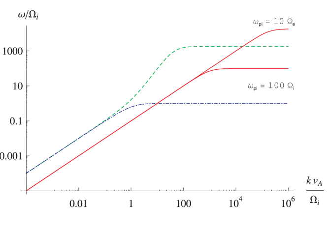
Figure 1: Dispersion relation of parallel-propagating plasma waves in low-beta plasma, i.e., for $c_{\mathrm{s}}/v_{\mathrm{A}}=0.1$. The red (solid) curves represent the ion sound wave for a high-density ($\omega_{\mathrm{pi}}=10\,\Omega_{\mathrm{e}}$) and low-density ($\omega_{\mathrm{pi}}=100\,\Omega_{\mathrm{i}}$) plasmas, the blue (dot-dashed) curve is the L wave and the green (dashed) curve the R wave. Note that the horizontal parts of the dispersion relation represent very strongly damped waves.

The first two interactions to be inspected are

$$\mathrm{L}^{+} \leftrightarrow \mathrm{I}^{+}+\mathrm{L}^{-}$$ (41)

$$\mathrm{R}^{+} \leftrightarrow \mathrm{I}^{+}+\mathrm{R}^{-}$$ (42)

which have been discussed under the MHD approximation already in [5]. They fulfill the resonance condition also in the dispersive limit up to the wave number, where $\omega_{\mathrm{T}}(k)\sim\omega_{\mathrm{Lo}}(k)$, so they are allowed in the low $\beta$-regime. We will analyse these reactions numerically below.

The interactions

$$\mathrm{L}^{+} \leftrightarrow \mathrm{L}^{+}+\mathrm{I}^{+}$$ (43)

$$\mathrm{R}^{+} \leftrightarrow \mathrm{R}^{+}+\mathrm{I}^{+}$$ (44)

can not fulfill the resonance conditions in the MHD regime, since in the low-frequency range the phase speed of the transverse waves is larger than that of the longitudinal wave for low $\beta$. The interaction involving the R-wave may work only if the decaying wave frequency is very close to $\omega_{\mathrm{R}}=\Omega_{\mathrm{e}}$, while the L-wave interaction is limited to work in a small frequency range close to $\Omega_{\mathrm{i}}$. We will analyse the reactions numerically below.

The L-wave reaction can be analysed analytically using the approximate dispersion relations,

$$k_{\mathrm{L}}(\omega) \approx \frac{\omega}{V_{\mathrm{A}}}\sqrt{\frac{\Omega_{\mathrm{i}}}{\Omega_{\mathrm{i}}-\omega}}$$ (45)

$$k_{\mathrm{I}}(\omega) \approx \frac{\omega}{c_{\mathrm{s}}}.$$ (46)

The resonance conditions yield

$$\frac{\omega}{V_{\mathrm{A}}}\sqrt{\frac{\Omega_{\mathrm{i}}}{\Omega_{\mathrm{i}}-\omega}}=\frac{\omega_{1}}{V_{\mathrm{A}}}\sqrt{\frac{\Omega_{\mathrm{i}}}{\Omega_{\mathrm{i}}-\omega_{1}}}+\frac{\omega-\omega_{1}}{c_{\mathrm{s}}},$$ (47)

where $\omega$ is the frequency of the decaying L wave and $\omega_{1}$ the frequency of the daughter L wave, $\omega-\omega_{1}$ being the frequency of the I wave. This condition can be written in the form $f(\omega/\Omega_{\mathrm{i}})=f(\omega_{1}/\Omega_{\mathrm{i}})$, where (Fig. 2)

$$f(x)=\frac{x}{\sqrt{\beta}}-\frac{x}{\sqrt{1-x}},\quad\beta=c^{2}_{\mathrm{s}}/V^{2}_{\mathrm{A}}$$ (48)

The function has two zeros at $x=0$ and $x=1-\beta$, and a positive value in betweenand a single maximum. The values of $\omega_{1}$ and $\omega$, thus, correspond to the two roots of the equation $f(\omega/\Omega_{\mathrm{i}})=C$, where $C$ is a constant between 0 and the maximum of $f$ which for a very low beta is at $x\approx 1-(\frac{1}{4}\beta)^{1/3}$. For higher values of $\beta$, the zero of the derivative, $x_{\textrm{max}}$, can be found by iteration taking $x_{\textrm{max}}^{(0)}=1-(\frac{1}{4}\beta)^{1/3}$ and

$$x_{\textrm{max}}^{(n+1)}=1-[\beta(\textstyle{\frac{1}{2}}x_{\textrm{max}}^{(n)}-1)^{2}]^{1/3},$$ (49)

Thus, one of the roots (the daughter wave $\omega_{1}$) is at $0<x<x_{\textrm{max}}$ and the other one (the decaying wave $\omega$) at $x_{\textrm{max}}<x<1-c_{\mathrm{s}}^{2}/V_{\mathrm{A}}^{2}$. The difference of the roots (multiplied by $\Omega_{\mathrm{i}}$) gives $\omega_{\mathrm{I}}$. This problem may be solved analytically, but the formula is of little practical use.

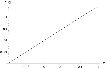
Figure 2: The function of $f(x)$ used to analyse the resonance conditions in the interaction $\mathrm{L}^{+}\leftrightarrow\mathrm{L}^{+}+\mathrm{I}^{+}$. The value of $\beta$ used in this plot is $\sim 0.0087$.

The R-wave reaction can be analysed in a similar manner, but the details are left to the interested reader.

By similar arguments, the three interactions

$$\mathrm{I}^{+} \leftrightarrow \mathrm{L}^{+}+\mathrm{R}^{+}$$ (50)

$$\mathrm{I}^{+} \leftrightarrow \mathrm{L}^{+}+\mathrm{R}^{-}$$ (51)

$$\mathrm{I}^{+} \leftrightarrow \mathrm{R}^{+}+\mathrm{L}^{-}$$ (52)

have no solution for the resonance condition in the low-frequency limit as the phase speed of the transverse waves exceeds the phase speed of the longitudinal wave. As above, however, this is no longer true in the direct vicinity of the resonances of the transverse waves.

For simplicity, we will consider a high-density plasma, for which a linear dispersion relation for the longitudinal wave is valid at all frequencies below $\Omega_{\mathrm{e}}$. The resonance conditions for the first two reactions yield

$$\frac{\omega_{\mathrm{L}}+\omega_{\mathrm{R}}}{c_{\mathrm{s}}}=k_{\mathrm{L}}(\omega_{\mathrm{L}})\pm k_{\mathrm{R}}(\omega_{\mathrm{R}}),$$ (53)

i.e.,

$$k_{\mathrm{L}}(\omega_{\mathrm{L}})-\frac{\omega_{\mathrm{L}}}{c_{\mathrm{s}}}=\frac{\omega_{\mathrm{R}}}{c_{\mathrm{s}}}\mp k_{\mathrm{R}}(\omega_{\mathrm{R}}),$$ (54)

The left-hand side is positive only for $k_{\mathrm{L}}>\Omega_{\mathrm{i}}/c_{\mathrm{s}}$. The right-hand side is always positive for the lower sign, interaction (51), and for the upper sign, interaction (50), as long as $k_{\mathrm{R}}<\Omega_{\mathrm{e}}/c_{\mathrm{s}}$. Similarly, for the third interaction (52) one can conclude that solutions are possible only for $k_{\mathrm{R}}>\Omega_{\mathrm{e}}/c_{\mathrm{s}}$. Thus, the following reactions are possible if $\omega_{\mathrm{pi}}>\Omega_{\mathrm{e}}$:

$$\mathrm{I}^{+} \leftrightarrow \mathrm{L}^{+}+\mathrm{R}^{+}\quad\mbox{for }k_{\mathrm{L}}>\Omega_{\mathrm{i}}/c_{\mathrm{s}}\mbox{ and }k_{\mathrm{R}}<\Omega_{\mathrm{e}}/c_{\mathrm{s}}$$ (55)

$$\mathrm{I}^{+} \leftrightarrow \mathrm{L}^{+}+\mathrm{R}^{+}\quad\mbox{for }k_{\mathrm{L}}<\Omega_{\mathrm{i}}/c_{\mathrm{s}}\mbox{ and }k_{\mathrm{R}}>\Omega_{\mathrm{e}}/c_{\mathrm{s}}$$ (56)

$$\mathrm{I}^{+} \leftrightarrow \mathrm{L}^{+}+\mathrm{R}^{-}\quad\mbox{for }k_{\mathrm{L}}>\Omega_{\mathrm{i}}/c_{\mathrm{s}}$$ (57)

$$\mathrm{I}^{+} \leftrightarrow \mathrm{R}^{+}+\mathrm{L}^{-}\quad\mbox{for }k_{\mathrm{R}}>\Omega_{\mathrm{e}}/c_{\mathrm{s}}.$$ (58)

Note that if $\omega_{\mathrm{pi}}<\Omega_{\mathrm{e}}$, interactions involving electron–cyclotron waves, Eqs. (56) and (58), are not possible at all, and the ranges of validity of the other reactions become modified (i.e., $\omega_{\mathrm{R}}<\omega_{\mathrm{pi}}-\Omega_{\mathrm{i}}$ needs to be satisfied).

In the reactions involving the ion-cyclotron waves, Eqs. (55) and (57), we may write $\omega_{\mathrm{L}}=\Omega_{\mathrm{i}}$ and get

$$k_{\mathrm{L}}=k_{\mathrm{I}}(\omega_{\mathrm{R}}+\Omega_{\mathrm{i}})\mp k_{\mathrm{R}}(\omega_{\mathrm{R}}),$$ (59)

which gives an analytical solution of the wave number of the left-handed wave as a function of the frequency of the right-handed wave. Note that this equation is valid also for $\Omega_{\mathrm{i}}<\omega_{\mathrm{pi}}<\Omega_{\mathrm{e}}$.

In summary, from the seven distinct possible interactions not eliminated by angular momentum conservation and $\mathrm{d}\omega/\mathrm{d}k>0$, only two can take place over the full frequency range in a low $\beta$-plasma with parallel wave propagation:

$$\mathrm{L}^{+} \leftrightarrow \mathrm{I}^{+}+\mathrm{L}^{-}$$

$$\mathrm{R}^{+} \leftrightarrow \mathrm{I}^{+}+\mathrm{R}^{-}.$$

In addition, the interactions (43)–(44) and (50)–(52) may have solutions where one of the waves are in the electron- or ion-cyclotron range. Reactions (43), (50) and (51) all yield solutions where an ion-cyclotron wave interacts with an MHD wave.

Numerical analysis.

For the two valid interactions and the one interaction with limited range we will now show the frequency triads for the resonance condition. As a model system for a low $\beta$ plasma we have chosen typical parameters for a coronal hole

Number density $$n_{\mathrm{i}}=n_{e}=2\times 10^{7}\,\mathrm{cm}^{-3}$$

Electron temperature $$T_{\mathrm{e}}=1\times 10^{6}\,\mathrm{K}$$

Magnetic field $$B=2\,\mathrm{G}$$

The values correspond to $\beta=c_{\mathrm{s}}^{2}/V_{\mathrm{A}}^{2}\approx 0.0087$ and $\omega_{\mathrm{pi}}/\Omega_{\mathrm{i}}\approx 310$.

In the upper right panel of Fig. 3 the interaction $\mathrm{I}^{+}+\mathrm{L}^{-}\leftrightarrow\mathrm{L}^{+}$ is shown. This interaction is very similar to the one described in [5], but for frequencies close to the ion gyrofrequency $\Omega_{\mathrm{i}}$ the effect of the L-wave resonance can be seen. At those frequencies, therefore, an ion-cyclotron wave is able to decay into a low-frequency Alfvén wave and a high-frequency ion sound wave. This process, however, has to compete against the dissipation of the mother wave due to ion cyclotron resonance.

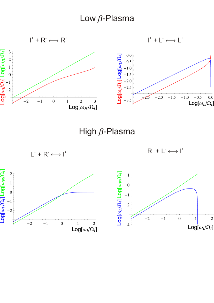
Figure 3: The frequencies of the daughter waves as a function of the frequency of the decaying wave in interactions, which fulfill the resonance condition in the whole frequency range including the MHD regime, analysed earlier in [2, 5]. In the plots L-waves (blue [dot-dashed] curve), R-waves (green [dashed] curve) and I-waves (red [solid] curve) can be seen.

The interaction $\mathrm{I}^{+}+\mathrm{R}^{-}\leftrightarrow\mathrm{R}^{+}$ (upper left panel of Fig. 3) is similar to the previous one in the low-frequency region, but shows a different behaviour for $\omega\geq\Omega_{\mathrm{i}}$, since the R-wave has no resonance there. The R-waves (the decaying one and the daughter wave) have a linear frequency relation, while the ion sound wave resembles the non-linear frequency difference due to the non-linear dispersion relation of the R-wave. It is noteworthy that the inverse cascading of the R-waves may proceed all they way from close to the electron-cycotron frequency through the Whistler range to the MHD regime.

In Fig. 4 the limited ranges of validity for the reactions $\mathrm{L}^{+}+\mathrm{I}^{+}\leftrightarrow\mathrm{L}^{+}$ and $\mathrm{I}^{+}\leftrightarrow\mathrm{L}^{+}+\mathrm{R}^{\pm}$ are plotted. The dispersive features of these new interactions are clearly visible.

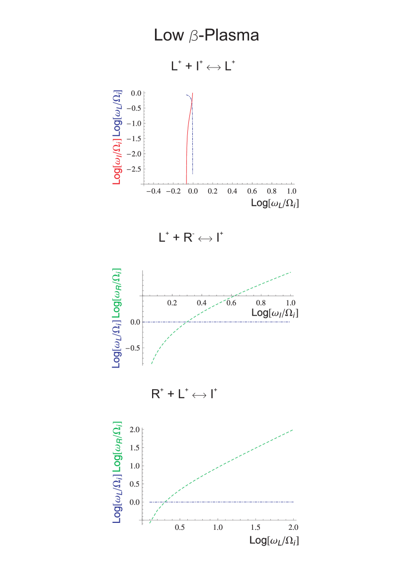
Figure 4: The frequencies of the daughter waves as a function of the frequency of the decaying wave in the new interactions, which fulfill the resonance conditions only in the dispersive wave regime in a low-beta plasma. In the plots L-waves (blue [dot-dashed] curve), R-waves (green [dashed] curve) and I-waves (red [solid] curve) can be seen.

3.2.2 High-$\beta$ Plasma

As we have done for the low $\beta$ case, we will also analyse the interactions with non-vanishing interaction coefficients for a high-beta plasma. We will, however, keep the discussion based on analytics more limited in this case than for the low-beta case. The dispersion relations in high-beta plasma are depicted in Fig. 5.

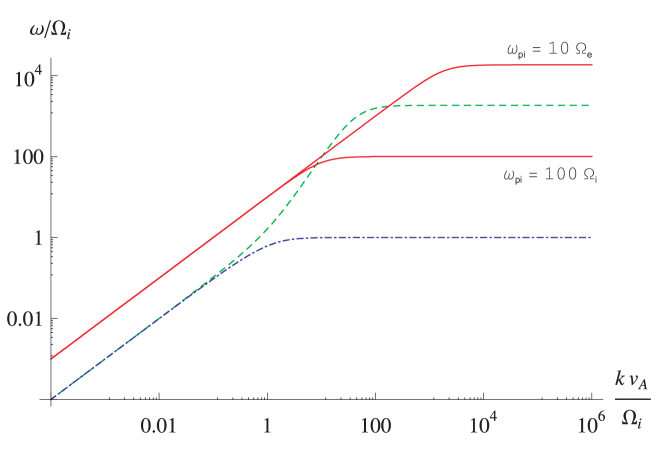
Figure 5: Dispersion relation of parallel-propagating plasma waves in high-beta plasma, i.e., for $c_{\mathrm{s}}/v_{\mathrm{A}}=10$. The red (solid) curves represent the ion sound wave for a high-density ($\omega_{\mathrm{pi}}=10\,\Omega_{\mathrm{e}}$) and low-density ($\omega_{\mathrm{pi}}=100\,\Omega_{\mathrm{i}}$) plasmas, the blue (dot-dashed) curve is the L wave and the green (dashed) curve the R wave.

For $\beta>1$, the interaction

$$\mathrm{I}^{+} \leftrightarrow \mathrm{R}^{+}+\mathrm{L}^{+}$$ (60)

cannot fulfill the resonance condition at low frequencies, as the phase speed of longitudinal wave is higher than that of both the transverse waves. However, if the ion sound speed is below the maximum value of the whistler phase speed ($\approx 20\,V_{\mathrm{A}}$) or if the plasma has a low-enough density so that $\omega_{\mathrm{pi}}<\Omega_{\mathrm{e}}$, the R-wave phase speed exceeds the sound-wave phase speed (Fig. 5) and reactions may occur.

The interaction

$$\mathrm{L}^{+}\leftrightarrow\mathrm{I}^{+}+\mathrm{L}^{-}$$ (61)

is not possible in a high-$\beta$ plasma, as $k_{\mathrm{L}}(\omega)-\omega/c_{\mathrm{s}}>0\;\forall\;\omega<\Omega_{\mathrm{i}}$ in a high-beta plasma, and this makes it impossible to fulfill the resonance condition. The interaction

$$\mathrm{L}^{+} \leftrightarrow \mathrm{I}^{+}+\mathrm{L}^{+}$$ (62)

will not work either, because $k_{\mathrm{L}}(\omega)-\omega/c_{\mathrm{s}}$ is a monotonically increasing function, which allows the resonance condition, $k_{\mathrm{L}}(\omega)-\omega/c_{\mathrm{s}}=k_{\mathrm{L}}(\omega_{1})-\omega_{1}/c_{\mathrm{s}}$, to be fulfilled only at $\omega_{\mathrm{I}}=\omega-\omega_{1}=0$.

However, the interactions

$$\mathrm{R}^{+}\leftrightarrow\mathrm{I}^{+}+\mathrm{R}^{\pm}$$ (63)

are possible as long as at least one of the R waves falls in to the dispersive frequency range. The resonance conditions for a linear sound wave, $\omega_{\mathrm{I}}=c_{\mathrm{s}}k_{\mathrm{I}}$, yield

$$k_{\mathrm{R}}(\omega)-\frac{\omega}{c_{\mathrm{s}}}=\pm k_{\mathrm{R}}(\omega_{1})-\frac{\omega_{1}}{c_{\mathrm{s}}}.$$ (64)

The upper sign corresponds to $g(y)=g(y_{1})$ with $y=\omega/\Omega_{\mathrm{e}}$ and (Fig. 6)

$$g(y)=\frac{y}{\sqrt{\beta}}-y\sqrt{\frac{m_{\mathrm{e}}/m_{\mathrm{i}}}{(m_{\mathrm{e}}/m_{\mathrm{i}}+y)(1-y)}},$$ (65)

which has zeros at $y=0$ and

$$y_{\pm} = \frac{1-m_{\mathrm{e}}/m_{\mathrm{i}}\pm\sqrt{(1-m_{\mathrm{e}}/m_{\mathrm{i}})^{2}-4(\beta-1)m_{\mathrm{e}}/m_{\mathrm{i}}}}{2}$$ (66)

$$y_{-} \approx (\beta-1)m_{\mathrm{e}}/m_{\mathrm{i}},\quad y_{+}\approx 1-\beta m_{\mathrm{e}}/m_{\mathrm{i}}$$ (67)

and a single minimum between 0 and $y_{-}$ and a single maximum between $y_{-}$ and $y_{+}$. Thus, R waves with frequencies $y$ above the position $y_{\textrm{max}}$ of the maximum are decaying into R waves with frequencies below $y_{\textrm{max}}$, analogously to the low-beta case $\mathrm{L}^{+}\leftrightarrow\mathrm{L}^{+}+\mathrm{I}^{+}$, but now the mother-wave frequency is very close to $\Omega_{\mathrm{e}}$. However, there is also another branch of interactions, which corresponds to the negative values of $g$. There, R waves with frequencies above the position $y_{\textrm{min}}$ of the minimum of $g$, i.e., with $y\in(y_{\textrm{min}},y_{-})$ are decaying into R waves at frequencies $y\in(0,y_{\textrm{min}})$. The value of $y_{\textrm{min}}$ can be found iteratively in a similar manner as $x_{\textrm{max}}$ for $f(x)$ above, since at $y<y_{-}\ll 1$ and with $x=m_{\mathrm{i}}y/m_{\mathrm{e}}$ we have

$$g = \frac{m_{\mathrm{e}}x}{m_{\mathrm{i}}}\left(\frac{1}{\sqrt{\beta}}-\frac{1}{\sqrt{1+x}}\right)$$ (68)

$$\frac{\mathrm{d}g}{\mathrm{d}y} = \frac{\mathrm{d}x}{\mathrm{d}y}\frac{\mathrm{d}g}{\mathrm{d}x}=\frac{1}{\sqrt{\beta}}-\frac{\frac{1}{2}x+1}{(1+x)^{3/2}}$$ (69)

giving, for $g^{\prime}(y_{\textrm{min}})=0$, an iterative formula: $x_{\textrm{min}}^{(0)}=1$ and

$$x_{\textrm{min}}^{(n+1)}=[\beta(\textstyle{\frac{1}{2}}x_{\textrm{min}}^{(n)}+1)^{2}]^{1/3}-1.$$ (70)

Thus, these solutions are found for mother-wave frequencies $\omega\in[x_{\textrm{min}}\Omega_{\mathrm{i}},(\beta-1)\Omega_{\mathrm{i}}]$.

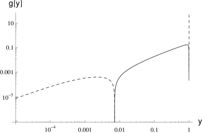
Figure 6: The function of $g(y)$ used to analyse the resonance conditions in the interaction $\mathrm{R}^{+}\leftrightarrow\mathrm{R}^{+}+\mathrm{I}^{+}$. The dashed curve gives $|g|$ for $g(y)<0$ and the solid curve the positive values of $g$. The value of $\beta$ used in this plot is $\sim 14$.

The lower sign in Eq. (64) yields solutions

$$\frac{y}{\sqrt{\beta}}-y\sqrt{\frac{m_{\mathrm{e}}/m_{\mathrm{i}}}{(m_{\mathrm{e}}/m_{\mathrm{i}}+y)(1-y)}}=\frac{y_{1}}{\sqrt{\beta}}+y_{1}\sqrt{\frac{m_{\mathrm{e}}/m_{\mathrm{i}}}{(m_{\mathrm{e}}/m_{\mathrm{i}}+y_{1})(1-y_{1})}},$$ (71)

meaning that the solutions are given by the roots of

$$g(y)=y_{1}\left(\frac{1}{\sqrt{\beta}}+\sqrt{\frac{m_{\mathrm{e}}/m_{\mathrm{i}}}{(m_{\mathrm{e}}/m_{\mathrm{i}}+y_{1})(1-y_{1})}}\right),$$ (72)

where the right-hand side is monotonic and can have any value between $0$ and $\infty$. Thus, this reaction involves mother-wave frequencies in the whole range where $g(y)$ is positive.

Finally, we are left with two interactions, which have been treated in [5] for the non-dispersive case

$$\mathrm{I}^{+} \leftrightarrow \mathrm{L}^{+}+\mathrm{R}^{-}$$ (73)

$$\mathrm{I}^{+} \leftrightarrow \mathrm{R}^{+}+\mathrm{L}^{-}.$$ (74)

These should work also in the dispersive case. We will analyse these reactions in more detail numerically.

Numerical analysis.

As for the low $\beta$-case we plot the solutions for the resonance condition in the high $\beta$-case. As a model system for a high $\beta$ plasma we have chosen parameters typical for the downstream region of a strong coronal shock

Number density $$n_{i}=n_{e}=8\times 10^{9}\,\mathrm{cm}^{-3}$$ (75)

Electron temperature $$T_{e}=2.5\times 10^{7}\,\mathrm{K}$$ (76)

Magnetic field $$B=5\,\mathrm{G}$$ (77)

The value of beta for this plasma is $\beta=c_{\mathrm{s}}^{2}/V_{\mathrm{A}}^{2}\approx 14$ and $\omega_{\mathrm{pi}}\approx 1.3\Omega_{\mathrm{e}}$.

The first interaction in the high-$\beta$ case has also been discussed in [5]: $\mathrm{I}^{+}\leftrightarrow\mathrm{L}^{+}+\mathrm{R}^{-}$ (lower left panel of Fig. 3). The solution of the resonance condition in the dispersive case is similar to the non-dispersive case for $\omega\leq\Omega_{\mathrm{i}}$. In the high-frequency regime we find, that the L-wave goes into resonance. For low frequencies the interaction takes place for an L-wave of slightly higher frequency than the R-wave, this changes at $\omega=\Omega_{\mathrm{i}}$. For high frequencies the energy is supplied almost completely by the R-wave, while the momentum comes from the L-wave.

The next interaction has also been discussed in [5]: $\mathrm{I}^{+}\leftrightarrow\mathrm{R}^{+}+\mathrm{L}^{-}$ (lower right panel of Fig. 3). Here the dispersive effects show a completely different behaviour. The L-wave frequency drops to zero for high frequencies, while the R-wave shows an almost linear increase.

For the interaction $\mathrm{R}^{+}\leftrightarrow\mathrm{R}^{+}+\mathrm{I}^{+}$ (top panel of Fig. 7) it can be clearly seen that there is only a small frequency band where the resonance condition can be fulfilled. This is due to phase speed of the R-wave which exceeds that of the sound wave only for a limited frequency range.

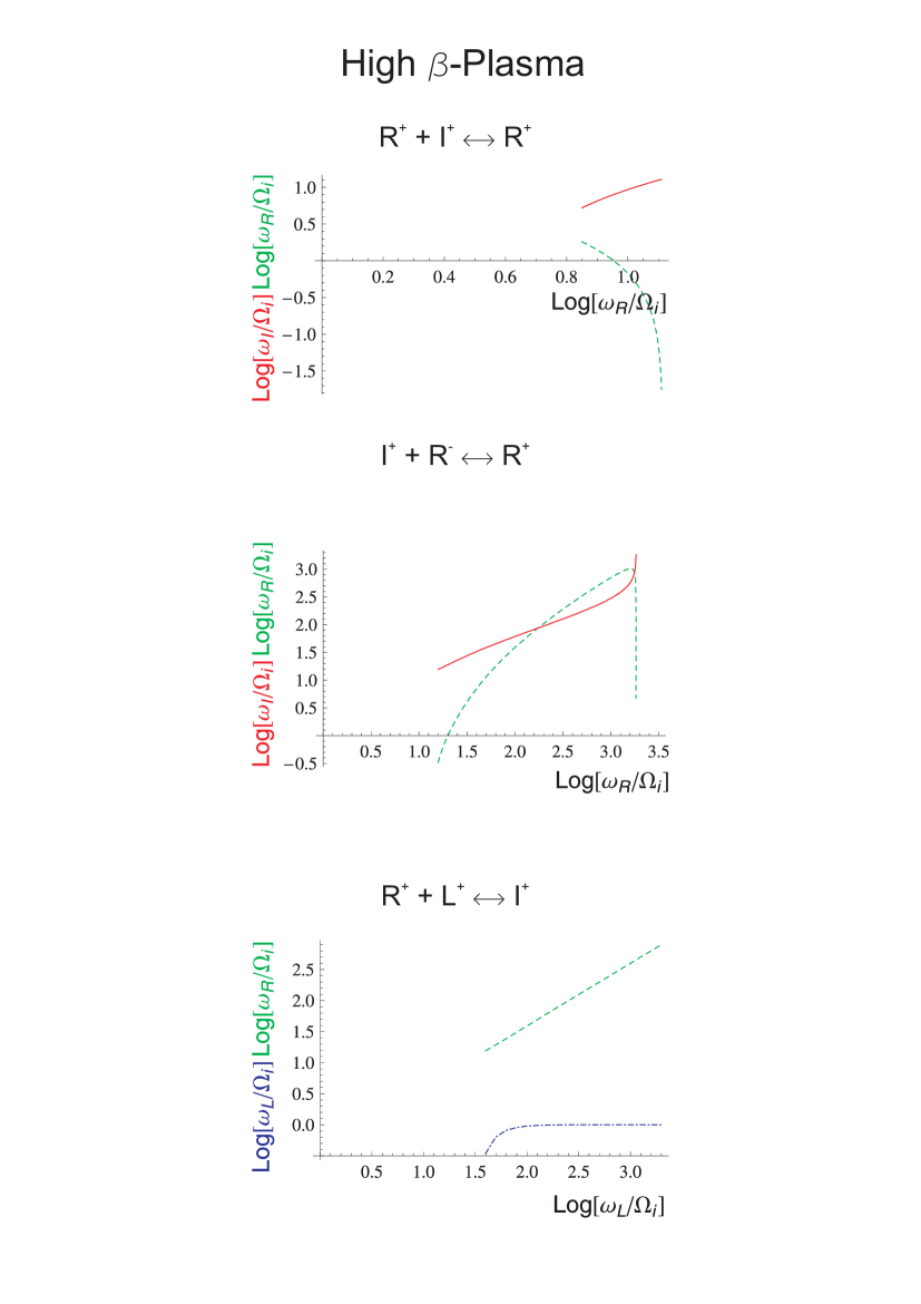
Figure 7: The frequencies of the daughter waves as a function of the frequency of the decaying wave in the new interactions, which fulfill the resonance conditions only in the dispersive wave regime in a high-beta plasma. In the plots L-waves (blue [dot-dashed] curve), R-waves (green [dashed] curve) and I-waves (red [solid] curve) can be seen.

As in the previous case, the interaction $\mathrm{R}^{+}\leftrightarrow\mathrm{I}^{+}+\mathrm{R}^{-}$ (middle panel of Fig. 7) shows clear dispersive effects. It is limited to the Whistler frequency range but has a larger range of validity than the previous case. In contrast to the previous case the upper limit is now given by the electron cyclotron limit of the R-wave.

Finally, the reaction $\mathrm{I}^{+}\leftrightarrow\mathrm{R}^{+}+\mathrm{L}^{+}$ is plotted in the bottom panel of Fig. 7. This shows that ion-cyclotron waves are able to interact with higher-frequency Whistlers propagating in the same direction, producing longitudinal waves that are rapidly damped. This reaction, thus, provides a dissipation mechanism for Whistlers in plasmas with cold ions and hot electrons.

4 Discussion and conclusions

We have analysed three-wave interactions of parallel-propagating plasma waves, concentrating on the effects of wave dispersion on the interactions. Our analysis shows that the theory is consistent with the conservation of angular momentum at microscopic level: the total amount of spin carried by the wave quanta must be conserved in the three-wave interactions. The reactions conserving the angular momentum are further analysed by employing the dispersion relations of left- and right-hand circularly polarised waves at frequencies below $\Omega_{\mathrm{i}}$ and $\Omega_{\mathrm{e}}$, respectively, and of ion-sound waves at frequencies below $\omega_{\mathrm{pi}}$.

Our analysis extends the previously analysed [2, 5] low-beta interactions,

$$\mathrm{L}^{+} \leftrightarrow \mathrm{I}^{+}+\mathrm{L}^{-}$$

$$\mathrm{R}^{+} \leftrightarrow \mathrm{I}^{+}+\mathrm{R}^{-}$$

to higher frequencies and shows that the latter reaction may occur also in high-beta plasma at Whistler frequencies of the mother R wave, where its phase speed exceeds that of the ion sound wave. The implied efficient inverse cascading of the R waves has important consequences on energetic particle transport and acceleration in collisionless plasmas: as higher-energy particles generally interact with lower-$k$ waves, this mechanism allows waves generated by low-energy particles to be converted to waves resonant with high energies, and this will enhance the rate of stochastic acceleration of the electrons, for example. Also the theory of diffusive shock acceleration (DSA) greatly benefits from an inverse cascade: it is the wave intensities at the lowest frequencies that determine the maximum energies produced in a shock in a given time, but as the upstream spectrum of plasma waves is usually generated by streaming instabilities due to the accelerated particles themselves, the spectrum of waves is usually an increasing function of frequency in the range resonant with the highest energy particles [10]. Obviously, an inverse cascade will increase the intensity of waves resonant with the highest energy particles and, therefore, increase the rate of acceleration.

The previously analysed high-beta interactions,

$$\mathrm{I}^{+} \leftrightarrow \mathrm{R}^{+}+\mathrm{L}^{-}$$

$$\mathrm{I}^{+} \leftrightarrow \mathrm{L}^{+}+\mathrm{R}^{-}$$

are also extended to higher frequencies. Both of these reactions are also possible in low-beta plasmas, as long as the frequency of the L wave is close to the ion-cyclotron frequency. As sound waves are rapidly damped in general, the reactions usually proceed to the direction of wave coalescence. Thus, these reactions may represent a new dissipation channel to the R waves in low-beta plasmas, although cyclotron damping of the L waves is also large near the resonance.

We have also discovered completely new interactions, which are not possible in an MHD description. In these reactions, all three waves propagate in the same direction,

$$\mathrm{I}^{+} \leftrightarrow \mathrm{R}^{+}+\mathrm{L}^{+}$$

$$\mathrm{L}^{+} \leftrightarrow \mathrm{L}^{+}+\mathrm{I}^{+}\quad(\mbox{low }\beta)$$

$$\mathrm{R}^{+} \leftrightarrow \mathrm{R}^{+}+\mathrm{I}^{+}\quad(\mbox{high }\beta),$$

which is strictly forbidden for non-dispersive waves. The latter two interactions shift energy from the dispersive frequency range to the MHD range, but an inverse cascade does not really develop, as the wave falls out of the frequency range able to decay already after the first interaction. This process, nevertheless, may help us understand, why spectrum of magnetic fluctuation in the solar wind experiences a clear break above the ion-cyclotron frequency [11], although the right-handed mode should not experience cyclotron damping in this frequency range.

Assuming that the sound waves are rapidly damped, all the discussed three-wave interactions provide a means of plasma heating. As the dissipation mechanism is not based on cyclotron resonance, the resulting heating rates on ions and electrons may be significantly different from direct ion-cyclotron damping.

In this paper, we only made use of the symmetries of the response tensor to find out the interactions with non-zero interaction rates. In a follow-up paper, we will study numerically the interaction rates of the three-wave interactions presented in this paper. This will allow us to deduce the importance of the interactions relative to other plasma phenomena, and determine the effects of three-wave interactions on plasma heating rates and particle acceleration.

In future work, it will also be important to extend the study also to waves propagating at a finite angle with respect to the magnetic field. In this case, as the polarisation tensor will become more complicated and the response tensor loses its transverse isotropy, many reactions should be allowed to occur. Another potentially important point to include to the model is multiple ion species. As the L waves will develop more resonances and subsequent cutoffs, especially the interactions $\mbox{L}^{+}\to\mbox{I}^{+}+\mbox{L}^{\pm}$ will be different from the ones presented here.

In conclusion, three-wave interactions in collisionless plasmas involving dispersive waves show a richer variety of possible reactions than the MHD counterparts. These reactions are potentially important in many branches of plasma astrophysics ranging from particle acceleration to plasma heating. We have identified some of them, but the theory has many more application not discussed in this paper.

References

- [1] D. Melrose, Instabilities in Space and Laboratory Plasmas, Cambridge University Press, Cambridge (1986)
- [2] Y.-C. Chin and D. G. Wentzel, Astrophysics and Space Sciences 16, 465–477 (1972)
- [3] D.G. Wentzel, Solar Physiscs 39, 129–140 (1974)
- [4] J. Skilling, Monthly Notes of the Royal astronomical Society 173, 255–269 (1975)
- [5] R. Vainio and F. Spanier, Astronomy and Astrophysics 437, 1–8 (2005)
- [6] Q. Luo and D. Melrose, Monthly Notes of the Royal astronomical Society 368, 1151–1158 (2006)
- [7] D. Melrose and W. Sy, Astrophysics and Space Sciences 17, 343–356 (1972)
- [8] D. Melrose and W. Sy, Australian J. Physics, 25, 387–402 (1972)
- [9] T.H. Stix, The Theory of Plasma Waves, McGraw-Hill, New York(1962)
- [10] R. Vainio and T. Laitinen, Astrophysical J., 658, 622–630 (2007)
- [11] K.U. Denskat, H.J. Beinroth, and F. M. Neubauer, 1983, J. Geophysics, 54, 60–67(1983)