Superfluid Bose-Fermi mixture from weak-coupling to unitarity

Abstract

We investigate the zero-temperature properties of a superfluid Bose-Fermi mixture by introducing a set of coupled Galilei-invariant nonlinear Schrödinger equations valid from weak-coupling to unitarity. The Bose dynamics is described by a Gross-Pitaevskii-type equation including beyond-mean-field corrections possessing the correct weak-coupling and unitarity limits. The dynamics of the two-component Fermi superfluid is described by a density-functional equation including beyond-mean-field terms with correct weak-coupling and unitarity limits. The present set of equations is equivalent to the equations of generalized superfluid hydrodynamics, which take into account also surface effects. The equations describe the mixture properly as the Bose-Bose repulsive (positive) and Fermi-Fermi attractive (negative) scattering lengths are varied from zero to infinity in the presence of a Bose-Fermi interaction. The present model is tested numerically as the Bose-Bose and Fermi-Fermi scattering lengths are varied over wide ranges covering the weak-coupling to unitarity transition.

I Introduction

The macroscopic quantum phenomenon of superfluidity has been clearly demonstrated in recent experiments with ultracold and dilute gases made of alkali-metal atoms stringa1 ; stringa2 . Both bosonic and fermionic ultracold and dilute superfluids can be accurately described by the zero-temperature hydrodynamical equations of superfluids stringa1 ; stringa2 ; landau1 ; landau2 ; leggett .

Trapped Bose-Fermi mixtures, with Fermi atoms in a single hyperfine state (normal Fermi gas), were investigated by various authors both theoretically molmer ; nygaard ; stoof ; pethick ; viverit1 ; viverit2 ; das ; liu ; wang and experimentally roati ; modugno ; ospelkaus . Recently, there was a study of a dilute mixture of superfluid bosons and fermions across a Feshbach resonance of the Fermi-Fermi scattering length $a_{f}$, obtaining the phase diagram of the mixture in a box sala-toigo . In the strict one-dimensional case, we found that the superfluid Bose-Fermi mixture exhibits phase separation and solitons by changing the Bose-Fermi interaction sala-sadhan-flavio ; md1 .

In the present paper we analyze in detail a 3D superfluid Bose-Fermi mixture under harmonic trapping confinement when the Bose-Bose repulsive (positive) and Fermi-Fermi attractive (negative) scattering lengths are varied from very small (weak coupling) to infinitely large (strong coupling) values. The variation of these scattering lengths from weak to strong coupling is achieved in laboratory fesh by varying a background magnetic field near a Feshbach resonance.

In the first part of the paper we derive Galilei-invariant nonlinear Schrödinger equations for superfluid Bose and Fermi dynamics, valid from weak-coupling to unitarity in each case, which are equivalent to the hydrodynamical equations. For bosons the equation is a generalized FP ; sala-ggpe ; sala-new zero-temperature Gross-Pitaevskii (GP) equation gross including beyond-mean-field corrections to incorporate correctly the effect of bosonic interaction for large and positive (repulsive) scattering lengths $a_{b}$. In the ordinary GP equation the nonlinear term is linearly proportional to $a_{b}$ and hence highly overestimates the effect of bosonic interaction for large positive values of $a_{b}$. In fact there is a saturation of bosonic interaction in the so-called unitarity $a_{b}\to+\infty$ limit, properly taken care of in the present generalized GP equations. For superfluid fermions the present formulation is based on the density-functional (DF) theory kohn1 ; kohn2 for fermion pairs kim ; manini05 ; adhikari ; sala-josephson ; sala-new including beyond-mean-field corrections to incorporate properly the effect of fermionic attraction between spin-up and down fermions specially for large negative (attractive) values of Fermi-Fermi scattering length $a_{f}$. The DF theory, in different forms, has already been applied to the problem of ultracold fermions kohn ; kohnx . The usual DF equation is valid for the weak-coupling Bardeen-Cooper-Schreiffer (BCS) limit: $a_{f}\to-0$. The present generalized DF equation correctly accounts for the dynamics as the Fermi-Fermi attraction is varied from the weak-coupling BCS limit to unitarity: $a_{f}\to-\infty$. In the unitarity limit there is a saturation of the effect of fermion interaction, properly taken care of in the present set of equations, which seems to be appropriate to study the crossover bcs-bose from the weak coupling BCS limit to the molecular Bose limit.

In the second part of the paper, by including the interaction between a boson and fermion pair, we obtain a set of coupled equation for superfluid Bose-Fermi dynamics in the presence of a Bose-Fermi interaction. The model correctly describes the dynamics as the Bose-Bose repulsion and Fermi-Fermi attraction are varied from weak-coupling to unitarity. This model is tested numerically as the different scattering lengths are varied over wide ranges covering the weak-coupling to unitarity transition for a superfluid Bose-Fermi mixture.

In Sec. II we present the hydrodynamical equations for bosons and fermions and present the appropriate bulk chemical potentials valid in the weak-coupling limit as well as possessing the saturation in the strong-coupling unitarity limit consistent with the constraints of quantum mechanics. In Sec. III we derive mean-field equations for bosons and fermions consistent with the hydrodynamical equations for a large number of atoms. Next we derive the present model for interacting Bose-Fermi superfluid introducing a contact interaction between bosons and fermions. In Sec. IV we perform numerical calculations for densities and chemical potentials of a trapped Bose-Fermi superfluid mixture to show the advantage of the present model. Finally, in Sec. V we present a brief summary and conclusion.

II Superfluid hydrodynamics for bosons and fermions

At zero temperature, for a large number of atoms, statical and dynamical collective properties of bosonic and fermionic superfluids are expected to be properly described by the hydrodynamical equations of superfluids stringa1 ; stringa2 . For bosons the hydrodynamical equations are given by stringa1 ; landau1

$${\partial\over\partial t}n_{b} + \nabla\cdot\left(n_{b}{\bf v}_{b}\right)=0\;,$$ (1)

$$m_{b}{\partial\over\partial t}{\bf v}_{b} + \nabla\left[{1\over 2}m_{b}v_{b}^{2}+U_{b}+\mu_{b}(n_{b},a_{b})\right]=0\;,$$ (2)

where $U_{b}({\bf r})$ is the external potential acting on bosons, $m_{b}$ is the mass of a bosonic atom, $n_{b}({\bf r},t)$ is the local density of bosons, and ${\bf v}_{b}({\bf r},t)$ is the local superfluid velocity stringa1 ; stringa2 ; landau1 . The total number of bosons is given by

$$N_{b}=\int n_{b}({\bf r},t)\ d^{3}{\bf r}\;,$$ (3)

and the nonlinear term $\mu_{b}(n_{b},a_{b})$ is the bulk chemical potential of the bosonic system with $a_{b}$ the Bose-Bose scattering length. Equation (1) is the equation of continuity of hydrodynamic flow, while Eq. (2) is the equation of conservation of the linear momentum. Equation (2) establishes the irrotational nature of the superfluid motion: $\nabla\wedge{\bf v}_{b}=0$, meaning that the velocity ${\bf v}_{b}$ can be written as the gradient of a scalar field. Equations (1) and (2) differ from the corresponding equations holding in the collisional regime of a non-superfluid system because of the irrotationality constraint.

For superfluid fermions, the fundamental entity governing the superfluid flow is the Cooper pair. In the case of a two-component (spin up and down) superfluid Fermi system one can introduce the local density of pairs $n_{p}({\bf r},t)=n_{f}({\bf r},t)/2$, where $n_{f}({\bf r},t)$ is the total local density of fermions. The hydrodynamical equations of a fermionic superfluid stringa2 ; landau1 ; landau2 ; leggett can be written as

$${\partial\over\partial t}n_{p} + \nabla\cdot\left(n_{p}{\bf v}_{p}\right)=0\;,$$ (4)

$$m_{p}{\partial\over\partial t}{\bf v}_{p} + \nabla\left[{1\over 2}m_{p}v_{p}^{2}+U_{p}+\mu_{p}(n_{p},a_{f})\right]=0\;,$$ (5)

where the nonlinear term $\mu_{p}(n_{p},a_{f})$ is the bulk chemical potential of pairs with $a_{f}$ the attractive Fermi-Fermi scattering length. Here $m_{p}$ is the mass of a pair, that is twice the mass $m_{f}$ of a single fermion, i.e. $m_{p}=2m_{f}$. In addition, the trap potential $U_{p}({\bf r})$ is twice the trap potential $U_{f}({\bf r})$ acting on a single fermion, i.e. $U_{p}({\bf r})=2U_{f}({\bf r})$. Note that the chemical potential $\mu_{p}(n_{p},a_{f})$ is twice the total chemical potential $\mu_{f}(n_{f},a_{f})$ of the Fermi system, i.e. $\mu_{p}(n_{p},a_{f})=2\mu_{f}(2n_{p},a_{f})$. The total number $N_{f}$ of fermions is

$$N_{f}=2N_{p}=2\int n_{p}({\bf r})\ d^{3}{\bf r}=\int n_{f}({\bf r})\ d^{3}{\bf r}\;,$$ (6)

where $N_{p}$ is the number of pairs.

It is important to stress that Eqs. (1) and (2) are formally similar to Eqs. (4) and (5), but the quantities involved are strongly different. In particular, the bulk chemical potential of bosons is completely different from the bulk chemical potential of Fermi pairs stringa1 ; stringa2 ; sala-ideal .

In the full crossover from the small-gas-parameter regime to the large-gas-parameter regime we use the following expression for the bulk chemical potential of the Bose superfluid sala-ggpe

$$\mu_{b}(n_{b},a_{b})=\frac{\hbar^{2}}{m_{b}}n_{b}^{2/3}f(n_{b}^{1/3}a_{b})\;,$$ (7)

where

$$f(x)=4\pi\frac{x+\alpha x^{5/2}}{1+\gamma x^{3/2}+\beta x^{5/2}}\;.$$ (8)

In the small-gas-parameter ($x\to 0$) regime, Eq. (8) becomes

$$f(x)=4\pi\left[x+(\alpha-\gamma)x^{5/2}+...\right],$$ (9)

which is the analytical result for bulk chemical potential found by Lee, Yang, and Huang LY ; LYH in this limit, provided that $(\alpha-\gamma)=32/(3\sqrt{\pi})$. In Eq. (8) we shall also choose $\beta=4\pi\alpha/\eta$, with $\eta=22.22$; this will make the bulk chemical potential (7) satisfy the correct unitarity limit $\mu_{b}(n_{b},a_{b})=22.22\hbar^{2}n_{b}^{2/3}/m_{b}$ as established by Cowell et al. cowell . Hence Eqs. (7) with (8) can be made to satisfy the correct weak-coupling and unitarity limits. Next we need to determine the constants $\alpha$ and $\gamma$ consistent with $(\alpha-\gamma)=32/(3\sqrt{\pi})$. We consider the following three choices for $\alpha$ and $\gamma$ from a possible many choices: $\alpha=32\nu/(3\sqrt{\pi})$, $\gamma=32(\nu-1)/(3\sqrt{\pi})$ with (a) $\nu=1.05$, (b) $\nu=1.1$, and (c) $\nu=1.15$. All three choices are consistent with the unitarity and the Lee-Yang-Huang limits LY ; LYH . We shall present a critical numerical study of the three choices in the next section.

In the full crossover from BCS regime ($a_{f}\to-0$) to unitarity ($a_{f}\to-\infty$) we use the following expression for the bulk chemical potential of the Fermi superfluid adhik

$$\mu_{p}(n_{p},a_{f})=2\frac{\hbar^{2}}{m_{p}}(6\pi^{2}n_{p})^{2/3}g(2^{1/3}n_{p}^{1/3}a_{f})$$ (10)

where

$$g(x)=1+\frac{\delta x}{1-\kappa x}\;,$$ (11)

where $\delta$ and $\kappa$ are fitting parameters. The close agreement of the interpolation function $g(x)$ for negative $x$ values with the results of Monte Carlo calculation of energy of a uniform gas of Fermi superfluid with the parameters $\delta=4\pi/(3\pi^{2})^{2/3}$, $\kappa=\delta/(1-\zeta)$, and $\zeta=0.44$ th1 ; th2 was established in Ref. adhik . The inclusion of the lowest-order term $g(x)=1$ in Eq. (10) leads to the bulk chemical potential in the absence of Fermi-Fermi interaction ($a_{f}=0$) of a uniform gas. The next-order term $g(x)=1+\delta x$ include known analytical result in the small-gas-parameter regime as obtained by Lee and Yang LY ; heisel and by Galitskii galit . The model (10) with (11) provides a smooth interpolation between the bulk chemical potential in the BCS limit $\mu_{p}(n_{p},a_{f})=2\hbar^{2}(6\pi^{2}n_{p})^{2/3}/m_{p}+{16}\pi n_{p}\hbar^{2}a_{f}/m_{p}$ LY for small $n_{p}^{1/3}a_{f}$ values and that in the unitarity limit adhik $\mu_{p}(n_{p},a_{f})=2\hbar^{2}(6\pi^{2}n_{p})^{2/3}\zeta/m_{p}$ for large $n_{p}^{1/3}a_{f}$ values. Manini and Salasnich manini05 and Kim and Zubarev kim also proposed similar interpolation formulas on the basis of Monte Carlo data of a uniform Fermi superfluid.

Here we deal with a Fermi gas in a spherical harmonic trap rather than a uniform Fermi gas. By a direct comparison with the results of Monte Carlo calculation of a superfluid Fermi gas in a spherical harmonic trap, we shall show in Sec. III that Eqs. (10) and (11) still present a good approximation to the bulk chemical potential of the system, but now with a slightly different value of the parameters.

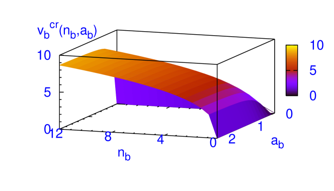
Figure 1: (Color online) The critical sound velocity $v_{b}^{cr}$ of a uniform Bose superfluid as a function of Bose-Bose scattering length $a_{b}$ and density $n_{b}$.

The hydrodynamical equations are valid to describe equilibrium properties and dynamical properties of long-wavelength for both bosons and fermions. In particular, one can introduce stringa1 ; stringa2 a healing (or coherence) length such that the transport phenomena under investigation must be characterized by a length scale much larger than the healing length. As suggested by Combescot, Kagan and Stringari combescot , the healing length can be defined for bosons as

$$\xi_{b}={\hbar\over m_{b}v_{b}^{cr}}\;,$$ (12)

where $v_{b}^{cr}$ is the Landau critical velocity above which the system gives rise to energy dissipation. This critical velocity coincides with the first sound velocity and is given by

$$v_{b}^{cr}=\sqrt{{n_{b}\over m_{b}}{\partial\mu_{b}\over\partial n_{b}}}\;.$$ (13)

In Fig. 1 we plot the critical sound velocity $v_{b}^{cr}$ of a uniform Bose superfluid for the present $\mu_{b}$ given by Eqs. (7) and (8) with the parameter $\nu=1.1$. The interesting feature of this plot is that $v_{b}^{cr}=0$, when either $n_{b}$ or $a_{b}$ is zero. However, $v_{b}^{cr}$ increases monotonically with $n_{b}$, whereas $v_{b}^{cr}$ attains a constant value as $a_{b}$ increases. These features are present in the plot of Fig. 1. However, the critical sound velocity $v_{b}^{cr}$ calculated from $\mu_{b}$ given by Eqs. (7) and (9) increases monotonically with both $n_{b}$ and $a_{b}$.

For superfluid fermions the healing length of Cooper pairs can be defined as

$$\xi_{p}={\hbar\over m_{p}v_{p}^{cr}}\;,$$ (14)

where the critical velocity $v_{p}^{cr}$ is related to the breaking of pairs through the formula

$$v_{p}^{cr}=\sqrt{\sqrt{\mu_{p}^{2}+|\Delta|^{2}}-\mu_{p}\over m_{p}}\;,$$ (15)

where $|\Delta|$ is the energy gap stringa2 ; combescot . We notice that in the deep BCS regime of weakly interacting attractive Fermi atoms (corresponding to $|\Delta|\ll\mu_{p}$) Eq. (15) approaches the exponentially small value $v_{p}^{cr}=|\Delta|/\sqrt{m_{p}\mu_{p}/2}$.

III Nonlinear Schrödinger equations

The bosonic superfluid can be described by a GP gross ; stringa1 complex order parameter $\Psi_{b}({\bf r},t)$ given by

$$\Psi_{b}({\bf r},t)=\sqrt{n_{b}({\bf r},t)}\ e^{i\theta_{b}({\bf r},t)}\ .$$ (16)

The probability current density $\vec{j}({\bf r},t)$ is given by

$$\vec{j}\equiv n_{b}{\bf v_{b}}=\frac{\hbar}{2im_{b}}(\Psi_{b}^{*}\nabla\Psi_{b}-\Psi_{b}\nabla\Psi_{b}^{*}).$$ (17)

Equations (16) and (17) relate the phase $\theta_{b}({\bf r},t)$ to the superfluid velocity field ${\bf v}_{b}$ by the formula stringa1 :

$${\bf v}_{b}={\hbar\over m_{b}}\nabla\theta_{b}\;.$$ (18)

The bosonic order parameter $\Psi_{b}({\bf r},t)$ is, apart from a normalization landau2 ; leggett , nothing but the condensate wave function

$$\Xi_{b}({\bf r},t)=\langle{\hat{\psi}}({\bf r},t)\rangle\;,$$ (19)

that is the expectation value of the bosonic field operator ${\hat{\psi}}({\bf r},t)$ landau2 ; sala-new . The order parameter $\Psi_{b}({\bf r},t)$ satisfies the following generalized GP nonlinear Schrödinger equation stringa1

$$i\hbar{\partial\over\partial t}\Psi_{b}=\left[-{\hbar^{2}\over 2m_{b}}\nabla^{2}+U_{b}+\mu_{b}(n_{b},a_{b})\right]\Psi_{b}\;,$$ (20)

where the bulk chemical potential is given by Eq. (7). The use of $f(x)=4\pi x$ in Eq. (7) leads to the GP equation and the use of the two leading terms of Eq. (9), e.g.,

$$f(x)=4\pi\left[x+{32\over 3\sqrt{\pi}}x^{5/2}\right]$$ (21)

in Eq. (7) leads to the modified GP (MGP) equation suggested by Fabrocini and Polls FP , which includes correction to the GP equation for medium values of Bose-Bose scattering length $a_{b}$. The use of Eq. (8) in Eq. (7) leads to a nonlinear Schrödinger equation valid from the weak-coupling to the unitarity limit and is called the unitary Schrödinger (US) equation for bosons sala-ggpe .

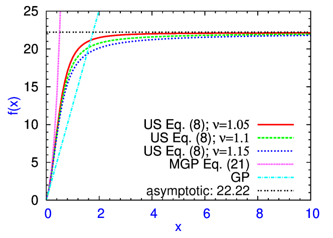
Figure 2: (Color online) The Bose interpolation function $f(x)$ given by Eq. (8) with $\alpha=32\nu/(3\sqrt{\pi}),\gamma=32(\nu-1)/(3\sqrt{\pi}),$ and $\beta=4\pi\alpha/22.22$ with $\nu=$ (a) 1.05, (b) 1.1, and (c) 1.15. The results of MGP [Eq. (21)] and GP [$f(x)=4\pi x$] models together with the asymptotic value are also given.

In Fig. 2 we plot the various possibilities for the interpolation function $f(x)$; e.g., those corresponding to the US equation (8) with (a) $\nu=1.05$, (b) $\nu=1.1$, and (c) $\nu=1.15$ [as suggested after Eq. (9)], the MGP equation (21), the GP equation $f(x)=4\pi x$. The asymptotic limit $\lim_{x\to\infty}f(x)=22.22$ is also shown. All three choices (a), (b), and (c) represent smooth interpolation of $f(x)$ between small and large $x$ values. For small $x$ this choice agrees with the MGP result (21) and for large $x$ with the asymptotic result. To test these three choices we actually solve the US Eq. (20), by imaginary time propagation after a Crank-Nicholson discretization num ; sala-numerics ; cn (detailed in the beginning of Sec. IV), for the trap parameters of a possible experimental set up for ⁸⁷Rb atoms in a spherical trap and compare the results for energy with those obtained by Blume and Greene bg by diffusion Monte Carlo (DMC) method. Actually, we solved Eqs. (20) and (7) with $n_{b}$ normalized to $(N_{b}-1)$ in place of Eq. (3), appropriate for a small number of bosons, cf. Eq. (2) of Ref. [48]. The energy of the system is calculated through a numerically constructed energy functional from the present bulk chemical potential. The calculation is performed for a boson-boson scattering length $a_{b}=0.433l$ where $l$ is the harmonic oscillator length for various $N_{b}$ and the results for energy are tabulated in Table 1. From this table we find that the present US models always provide a much better approximation to the energies than the GP and MGP models. More results of energy for larger number of bosons may help in fixing the parameters of the present model more accurately. In the present paper we shall use the US model (b) with $\nu=1.1$.

Table 1: Ground state energies for different number $N_{b}$ of bosonic atoms in a spherical trap and for $a_{b}=0.433$ from a solution of GP equation, MGP equation and US equation for $\nu$ = (a) 1.05, (b) 1.1 and (c) 1.15. The results for energies obtained with two potentials of DMC calculation bg are quoted for comparison. Length and energies are expressed in oscillator units.

$N_{b}$	DMC	GP	MGP	US (a)	US(b)	US(c)
3	5.553(3); 5.552(2)	5.329	5.611	5.570	5.564	5.558
5	10.577(2); 10.574(4)	9.901	10.772	10.629	10.608	10.588
10	26.22(8); 26.20(8)	23.61	26.84	26.24	26.16	26.07
20	66.9(4); 66.9(1)	57.9	68.5	66.38	66.07	65.77

The relationship between Eq. (20) and the hydrodynamical equations (1) and (2) can be established by inserting Eq. (16) into Eq. (20). After some straightforward algebra equating the real and imaginary parts of both sides and taking into account Eq. (18), one finds two generalized hydrodynamical equations stringa1

$${\partial\over\partial t}n_{b} + \nabla\cdot\left(n_{b}{\bf v}_{b}\right)=0\;,$$ (22)

$$m_{b}{\partial\over\partial t}{\bf v}_{b} + \nabla\biggr{[}-{\hbar^{2}\over 2m_{b}}{\nabla^{2}\sqrt{n_{b}}\over\sqrt{n_{b}}}+{m_{b}v_{b}^{2}\over 2}+\ U_{b}$$ (23)

$$+ \ \mu_{b}(n_{b},a_{b})\biggr{]}=0\;,$$

which include the quantum pressure term

$$T_{b}^{QP}=-{\hbar^{2}\over 2m_{b}}{\nabla^{2}\sqrt{n_{b}}\over\sqrt{n_{b}}}\;,$$ (24)

which depends explicitly on the reduced Planck constant $\hbar$. Neglecting the quantum pressure term, one gets from Eqs. (22) and (23) the classical hydrodynamical equations (1) and (2). Equation (22) is the continuity equation whereas Eq. (23) establishes the irrotational nature of hydrodynamic flow.

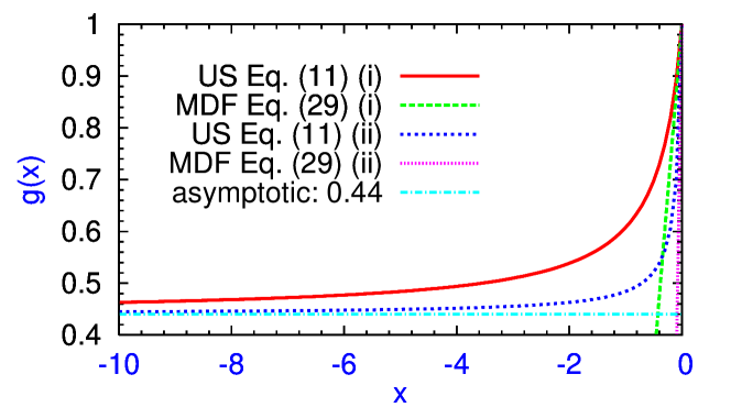
Figure 3: (Color online) The Fermi interpolation function $g(x)$ given by Eq. (11) with (i) $\delta=$ $4\pi/(3\pi^{2})^{2/3},$ and (ii) $20\pi/(3\pi^{2})^{2/3}$ and $\kappa=\delta/0.56$. The MDF results given by Eq. (29) and the asymptotic value are also shown.

Similarly, the fermionic superfluid can be described by a DF kohn complex order parameter $\Psi_{p}({\bf r},t)$ of pairs, with a modulus and a phase $\theta_{p}({\bf r},t)$ such that

$$\Psi_{p}({\bf r},t)=\sqrt{n_{p}({\bf r},t)}\ e^{i\theta_{p}({\bf r},t)}\;.$$ (25)

The expression for the probability current density of fermions leads to the following expression for the velocity field ${\bf v}_{p}$ of pairs stringa2 :

$${\bf v}_{p}={\hbar\over m_{p}}\nabla\theta_{p}\;.$$ (26)

Note that the mass of a pair $m_{p}$, and not that of a fermion, appears in the denominator of the phase-velocity relation. The fundamental entity responsible for superfluid flow has the mass $m_{p}$ of a pair of fermions. For paired fermions in the superfluid state, the order parameter is, apart from a normalization landau2 ; leggett ; sala-odlro , the condensate wave function of the center of mass of the Cooper pairs:

$$\Xi_{p}({\bf r},t)=\langle{\hat{\psi}}_{\uparrow}({\bf r},t){\hat{\psi}}_{\downarrow}({\bf r},t)\rangle\;,$$ (27)

that is the average of pair operators, with ${\hat{\psi}}_{\sigma}({\bf r},t)$ the fermionic field operator with spin component $\sigma=\uparrow,\downarrow$ landau2 ; sala-new . The order parameter $\Psi_{p}({\bf r},t)$ satisfies the following zero-temperature nonlinear DF Schrödinger equation kim ; manini05 ; sala-josephson ; sala-new ; adhik

$$i\hbar{\partial\over\partial t}\Psi_{p}=\left[-{\hbar^{2}\over 2m_{p}}\nabla^{2}+\ U_{p}+\ \mu_{p}(n_{p},a_{f})\right]\Psi_{p}\;,$$ (28)

where the bulk chemical potential $\mu_{p}(n_{p},a_{f})$ is given by Eq. (10). The use of $g(x)=1$ in $\mu_{p}(n_{p},a_{f})$ of Eq. (10) leads to the lowest order DF equation. If we use the next order solution of Eq. (11) in Eq. (10), e. g.,

$$g(x)=1+\delta x,$$ (29)

we obtain a modified density-functional (MDF) equation with corrections for medium values Fermi-Fermi scattering length $a_{f}$. The use of Eq. (11) in Eq. (10) leads to a DF equation valid in the weak-coupling BCS to unitarity limit and the resultant nonlinear equation (28) will be called the unitary Schrödinger (US) equation for fermion pairs.

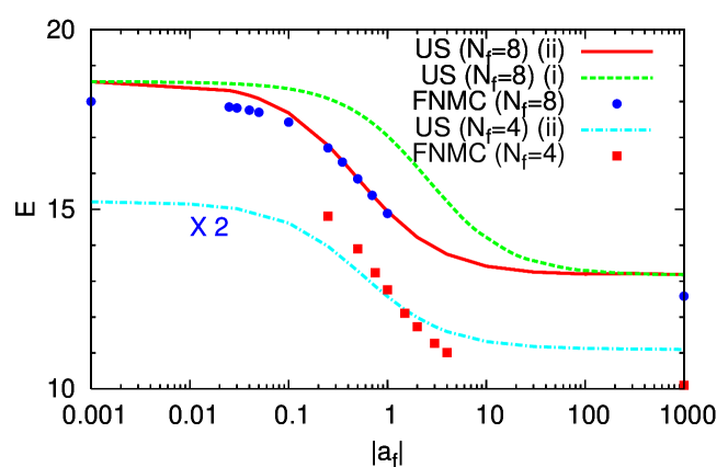
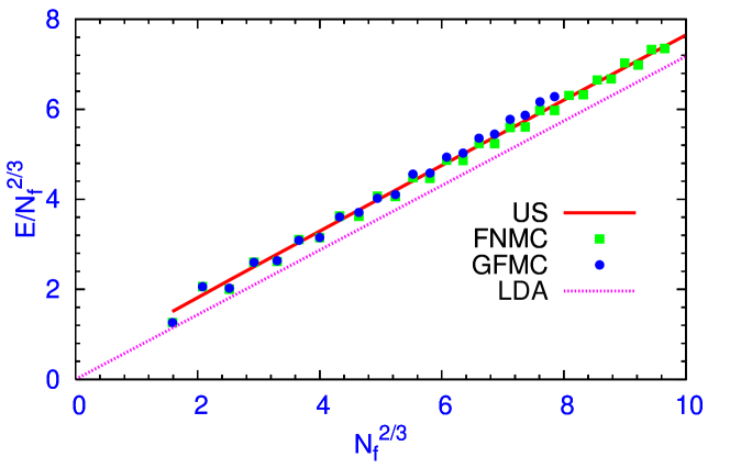
Figure 4: (Color online) (a) Energy of a superfluid Fermi gas in a spherical trap in oscillator units vs. Fermi-Fermi scattering length $a_{f}$ also in oscillator units obtained from the solution of Eq. (28) for the choices $\delta=$ (i) $4\pi/(3\pi^{2})^{2/3}$ and (ii) $20\pi/(3\pi^{2})^{2/3}$ and from the fixed node Monte Carlo (FNMC) calculation FNMC ; FNMC2 . (b) Energy of a superfluid Fermi gas in a spherical trap in oscillator units vs. number of atoms $N_{f}$ in the unitarity limit $a_{f}\to-\infty$ obtained from a solution of Eq. (28), from FNMC FN and Green function Monte Carlo (GFMC) calculations GFMC , and from local density approximation (LDA).

In Fig. 3 we plot the various possibilities for the interpolation function $g(x)$; e. g., that corresponding to Eq. (11), the MDF equation (29) for two different values of $\delta$: (i) $4\pi/(3\pi^{2})^{2/3}$ and (ii) $20\pi/(3\pi^{2})^{2/3}$. The parameter $\kappa$ is always taken as $\kappa=\delta/(1-\zeta),$ $\zeta=0.44$ th1 ; th2 . The asymptotic limit $\lim_{x\to\infty}g(x)=0.44$ is also shown in Fig. 3. The expression (11) represents a good approximation of $g(x)$ for small and large $|x|$. For small $|x|$ this choice agrees with the MDF result (29) and for large $|x|$ with the asymptotic result for both choices of $\delta$.

To test the above two choices (i) and (ii) of the parameter $\delta$ in Eq. (11) for a Fermi superfluid in a spherical trap, we calculate the energy of the system for different values of the scattering length $a_{f}$ and number of atoms $N_{f}$ by solving directly Eq. (28) by imaginary time propagation after a Crank-Nicholson discretization num ; sala-numerics ; cn (detailed in the beginning of Sec. IV). We also compare the results with those obtained by the fixed-node Monte Carlo calculation (FNMC) FN ; FN2 ; FNMC ; FNMC2 . The results of our investigation are shown in Figs. 4. In Fig. 4 (a) we plot energy $E$ vs. $|a_{f}|$ for $N_{f}=4$ and 8 obtained from a solution the US equation (28) with the choices (i) $4\pi/(3\pi^{2})^{2/3}$ and (ii) $20\pi/(3\pi^{2})^{2/3}$ for $\delta$ and the FNMC data of Ref. FNMC ; FNMC2 . The present hydrodynamical formulation is expected to be good for for a large number of fermions [see, Fig. 4 (b)], yet for a small number $N_{f}=4$ the result is reasonable. In Fig. 4 (b) we plot energy $E/N_{f}^{2/3}$ vs. $N_{f}^{2/3}$ at unitarity $a_{f}\to-\infty$ obtained from a solution of the US equation (28) with choice (ii) $20\pi/(3\pi^{2})^{2/3}$ for $\delta$. In this limit both choices of $\delta$ lead to the same energy. The results of FNMC FN and Green function Monte Carlo (GFMC) GFMC calculations as well as of LDA are also shown in Fig. 4 (b). The LDA result is analytically known in this case as $E(N)=(3N_{f})^{4/3}\sqrt{\xi}/4,\xi=0.44$ kohnx . We plot $E/N_{f}^{2/3}$ vs. $N_{f}^{2/3}$ in Fig. 4 (b) because of the linear correlation between these two variables explicit in the LDA result. From Figs. 4 we find that the results with choice (ii) $20\pi/(3\pi^{2})^{2/3}$ of $\delta$ agree well with the Monte Carlo data in both cases and this choice will be used in the present study. The Monte Carlo data clearly favors the present model over the LDA.

Again, inserting Eq. (25) into Eq. (28), after some straightforward algebra equating the real and imaginary parts and taking into account Eq. (26), we find two generalized hydrodynamical equations for the Fermi superfluid

$${\partial\over\partial t}n_{p} + \nabla\cdot\left(n_{p}{\bf v}_{p}\right)=0\;,$$ (30)

$$m_{p}{\partial\over\partial t}{\bf v}_{p} + \nabla\biggr{[}-{\hbar^{2}\over 2m_{p}}{\nabla^{2}\sqrt{n_{p}}\over\sqrt{n_{p}}}+{m_{p}v_{p}^{2}\over 2}+\ U_{p}$$ (31)

$$+ \ \mu_{p}(n_{p},a_{f})\biggr{]}=0\;,$$

which include the quantum pressure term

$$T_{p}^{QP}=-{\hbar^{2}\over 2m_{p}}{\nabla^{2}\sqrt{n_{p}}\over\sqrt{n_{p}}}\;,$$ (32)

involving $\hbar$. Neglecting this term leads to the classical hydrodynamical equations (4) and (5) of superfluid Fermi pairs. This specific quantum pressure term is a consequence of the proper phase-velocity relation (26) with the factor $m_{p}$ in the denominator stringa2 . Had we taken a different mass factor in the denominator, e.g. $m_{f}$, a different quantum pressure term would have emerged. The present choice is physically motivated by Galilei invariance stringa2 ; sala-josephson ; sala-new and leads to energies of trapped Fermi superfluid in close agreement adsa with those obtained FN ; GFMC from the Monte Carlo methods.

We stress that, from the point of view of DF theory, the quantum pressure terms for superfluid bosons and fermions correspond to gradient correction (also called surface corrections) to the local density approximation (LDA), where LDA gives exactly the classical hydrodynamical equations obtained by setting gradient kinetic-energy term to zero. The gradient term, which can also be seen as a next-to-leading contribution in a momentum expansion to the classical superfluid hydrodynamics son , takes into account corrections to the kinetic energy due to spatial variations in the density of the system, and it is essential to have regular behavior at the surface of the cloud where the density goes to zero tosi . In the case of superfluid bosons, the quantum-pressure term, Eq. (24), is exactly the one of the familiar cubic GP equation stringa1 ; gross . In the case of superfluid fermions the gradient term is consistent with the motion of paired fermions of mass $m_{p}=2m_{f}$. For normal fermions various authors have proposed and used different gradient terms von ; tosi ; zaremba ; sala-gradient ; adhikari2 . For superfluid fermions we are using the familiar von Weizsäcker term von in the case of pairs. In fact, in our approach, the explicit form of the quantum-pressure term, Eq. (32), is strictly determined by the Galilei-invariant relation, Eq. (26), between phase and superfluid velocity stringa2 ; sala-josephson ; sala-new . Finally, we observe that Eq. (32) is practically the same as that recently obtained in Ref. save-us in the case of a superfluid Fermi gas at unitarity using an $\epsilon$ expansion around $d=4-\epsilon$ spatial dimensions.

The generalized hydrodynamical equations (22) and (23) for bosons and (30) and (31) for fermions are thus completely equivalent to the respective nonlinear Schrödinger equations (20) and (28). In the limit of zero velocity fields, ${\bf v}_{b},{\bf v}_{p}\to 0$, Eqs. (23) and (31) yield the stationary versions of Eqs. (20) and (28) describing the superfluid densities:

$$\mu_{b0}\sqrt{n_{b}}=\left[-{\hbar^{2}\over 2m_{b}}\nabla^{2}+\ U_{b}+\ \mu_{b}(n_{b},a_{b})\right]\sqrt{n_{b}}\;,$$ (33)

$$\mu_{p0}\sqrt{n_{p}}=\left[-{\hbar^{2}\over 2m_{p}}\nabla^{2}+\ U_{p}+\ \mu_{p}(n_{p},a_{f})\right]\sqrt{n_{p}}\;,$$ (34)

showing the agreement between hydrodynamical and nonlinear equations for superfluid bosons and fermions. Here $\mu_{b0}$ and $\mu_{p0}$ are the chemical potentials for bosons and fermions in the stationary state.

Although Eq. (34) is written in terms of Fermi pair density $n_{p}$ (and we use this equation in the following), an equivalent equation for Fermi density $n_{f}$ (=2$n_{p}$) can be written as

$$\mu_{f0}\sqrt{n_{f}}=\left[-{\hbar^{2}\over 8m_{f}}\nabla^{2}+\ U_{f}+\ \mu_{f}(n_{f},a_{f})\right]\sqrt{n_{f}}\;,$$ (35)

$$\mu_{f}(n_{f},a_{f})=\frac{\hbar^{2}}{2m_{f}}(3\pi^{2}n_{f})^{2/3}g(n_{f}^{1/3}a_{f})\;,$$ (36)

where we have used $\mu_{p0}=2\mu_{f0}$, $U_{p}=2U_{f},$ and $\mu_{p}(n_{p},a_{f})=2\mu_{f}(n_{f},a_{f}).$

Equations (20) and (28) are the Euler-Lagrange equations of the following Lagrangian density

$${\cal L}_{j} = {i\hbar\over 2}\left(\Psi_{j}^{*}{\partial\over\partial t}\Psi_{j}-\Psi_{j}{\partial\over\partial t}\Psi_{j}^{*}\right)-{\hbar^{2}\over 2m_{j}}|\nabla\Psi_{j}|^{2}$$ (37)

$$- U_{j}({\bf r})|\Psi_{j}|^{2}-{\cal E}_{j}(n_{j},a_{j})|\Psi_{j}|^{2}\;,$$

with $j=b,p$, (here $a_{p}=a_{f}$, the Fermi-Fermi scattering length) where

$${\cal E}_{j}(n_{j},a_{j})={1\over n_{j}}\int_{0}^{n_{j}}\mu_{j}(n^{\prime}_{j},a_{j})\ dn^{\prime}_{j}\;,$$ (38)

is the bulk energy per particle of the superfluid.

Finally, we introduce a Lagrangian density for Bose-Fermi interaction to (37) of the form

$${\cal L}_{bp}=G_{bp}|\Psi_{b}|^{2}|\Psi_{p}|^{2},$$ (39)

where $G_{bp}={4\pi\hbar^{2}a_{bf}}/{m_{bf}}$, and $m_{bf}$ is the Bose-Fermi reduced mass and $a_{bf}$ the Bose-Fermi scattering length.

We note that there are no coupling terms between the hydrodynamical equations (23) and (31) involving the velocity of two superfluid components. The only coupling in the Lagrangian density (39) involves the density of the two superfluid components. However, the present hydrodynamical equations (23) and (31) are a special case of the three-fluid (two superfluids and a normal fluid) hydrodynamical formulation of Landau and Khalatnikov landau3 (appropriate for the ⁴He-³He mixture). The Galilei-invariant Landau-Khalatnikov formulation in its general form also has a coupling term involving two superfluid velocities (not considered in this paper), as discussed landau4 by Andreev and Bashkin and also by Ho and Shenoy. However, the present static model defined by Eqs. (33) and (34) is obtained by setting all velocities equal to zero, and hence, these terms depending on superfluid velocities would leave the present model unchanged.

In this paper we consider $a_{bf}$ to have not too large positive values only (moderately repulsive Bose-Fermi interaction.) There are other domains of Bose-Fermi interaction which require special attention. If this interaction is attractive and strong enough, then the ground state is very different, e.g., the composite fermions $\tilde{f}=bf$ are created at higher temperatures and at zero temperature we have Cooper pairs (or local pairs) of the type $<\tilde{f}\mbox{ }\tilde{f}>$ consisting of two elementary fermions and two elementary bosons kagan .

The complete Lagrangian density given by Eqs. (37) and (39) leads to the following set of coupled equations for the Bose-Fermi-Fermi mixture made of superfluid bosons and two-component superfluid fermions

$$i\hbar{\partial\over\partial t}\Psi_{b} = \left[-{\hbar^{2}\nabla^{2}\over 2m_{b}}+U_{b}+\mu_{b}(n_{b},a_{b})+G_{bp}|\Psi_{p}|^{2}\right]\Psi_{b}\;,$$

$$i\hbar{\partial\over\partial t}\Psi_{p} = \left[-{\hbar^{2}\nabla^{2}\over 2m_{p}}+U_{p}+\mu_{p}(n_{p},a_{f})+G_{bp}|\Psi_{b}|^{2}\right]\Psi_{p}\;,$$

valid from weak-coupling to unitarity for both bosons and fermions. The coupled set of equations (III) and (III) with bulk chemical potentials $\mu_{b}(n_{b},a_{b})$ and $\mu_{p}(n_{p},a_{f})$ given by Eqs. (7) and (8) (with $\nu=1.1$) and Eqs. (10) and (11) [with $\delta=20\pi/(3\pi^{2})^{2/3},\kappa=\delta/(1-\zeta),\zeta=0.44$], respectively, is the US equation for the interacting superfluid Bose-Fermi mixture and is the required set. However, when the bulk chemical potentials $\mu_{b}(n_{b},a_{b})$ and $\mu_{p}(n_{p},a_{f})$ are approximated using Eqs. (21) and (29), the set of equations (III) and (III) will be termed modified Gross-Pitaevskii density-functional (MGPDF) equation including some correction for medium values of scattering lengths $a_{b}$ and $a_{f}$. Finally, if we approximate $f(x)=4\pi x$ and $g(x)=1$ in Eqs. (III) and (III) with Eqs. (8) and (11), the resultant model is termed Gross-Pitaevskii density-functional (GPDF) model. We present a comparative numerical study of these three models $-$ US, MGPDF, and GPDF $-$ in the next section.

IV Numerical Results

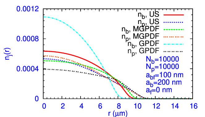
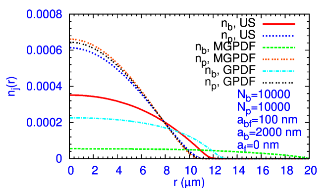
Figure 5: (Color online) The normalized densities $n_{j}(r)=|\Psi_{j}|^{2}$ with $j=b,p$ from a solution of Eqs. (III) and (III) for the US, MGPDF, and GPDF models with $N_{b}=10000,N_{p}=10000,a_{bf}=100$ nm, $a_{f}=0$, and (a) $a_{b}=200$ nm, and (b) $a_{b}=2000$ nm. In this plot $\int n_{j}({\bf r})d^{3}{\bf r}=1.$

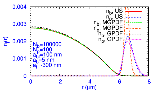
Figure 6: (Color online) The normalized densities $n_{j}(r)=|\Psi_{j}|^{2}$ with $j=b,p$ from a solution of Eqs. (III) and (III) for the US, MGPDF, and GPDF models with $N_{b}=100000,N_{p}=100,a_{bf}=100$ nm, $a_{b}=5$ nm, and (a) $a_{f}=-100$ nm, and (b) $a_{bf}=-300$ nm. In this plot $\int n_{j}({\bf r})d^{3}{\bf r}=1.$

Here we solve numerically the coupled set of US Eqs. (III) and (III) with bulk chemical potentials $\mu_{b}$ and $\mu_{p}$ given by Eqs. (8) and (11) and compare the results so obtained with those of the MGPDF and GPDF models. We numerically solve the US, MGPDF, and GPDF partial differential equations by discretizing them by the semi-implicit Crank-Nicholson algorithm with imaginary time propagation num ; sala-numerics ; cn . The space and time steps used in discretization were typically 0.05 and 0.001 respectively.

Although we are not interested here in fitting experimental data, we perform numerical calculation for variables for a possible experimental set up modugno of ⁸⁷Rb-⁴⁰K mixture in spherical harmonic traps satisfying $U_{b}=m_{b}\omega_{b}^{2}r^{2}/2=m_{f}\omega_{f}^{2}r^{2}/2=U_{f}$ with an oscillator length $l=\sqrt{\hbar/{(m_{b}\omega_{b})}}=1$ $\mu$m for ⁸⁷Rb atoms. The oscillator length for ⁴⁰K is modified according to the trap. The fermion pair trap in Eq. (III) is $U_{p}=m_{f}\omega_{f}^{2}r^{2}$.

In Figs. 5 (a) and (b) we plot densities for the superfluid Bose-Fermi mixture as calculated from Eqs. (III) and (III) for $N_{b}=10000,N_{p}=10000,a_{f}=0,a_{bf}=100$ nm with (a) $a_{b}=200$ nm and (b) $a_{b}=2000$ nm for the US, MGPDF, and GPDF models. For small $a_{b}$ both MGPDF, and GPDF models are good approximations to the bosonic density of the US model (not shown in figure). But as $a_{b}$ increases, the MGPDF model is a better approximation to the bosonic density of the US model than the GPDF model as can be seen from Fig. 5 (a). However, for very large $a_{b}$, neither the MGPDF nor the GPDF model provides the saturation of bulk chemical potential for bosons as in the US model. Consequently, the MGPDF, and GPDF models acquire large bosonic nonlinearity compared to the US model and hence produce bosonic density extending to larger region in space. As $a_{b}$ is increased, the MGPDF model yields rapidly divergent bosonic nonlinearity (compared to the GPDF model) and hence produces bosonic density inferior to the GPDF model as can be seen in Fig. 5 (b).

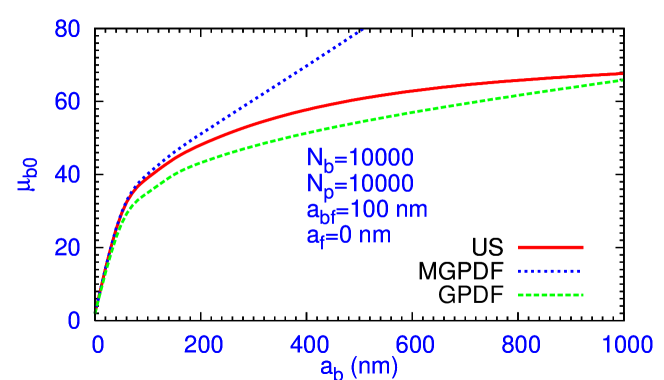
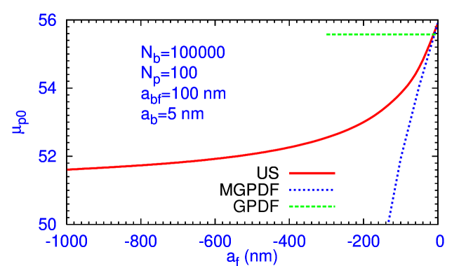
Figure 7: (Color online) (a) Chemical potential $\mu_{b0}$ vs. $a_{b}$ of Eqs. (33) and (34) for the US, MGPDF, and GPDF models for $N_{b}=N_{p}=10000,a_{f}=0,a_{bf}=100$ nm and (b) chemical potential $\mu_{p0}$ vs. $a_{f}$ for the US, MGPDF, and GPDF models for $N_{b}=100000,N_{p}=100,a_{b}=5$ nm, $a_{bf}=100$ nm, respectively. The chemical potentials are expressed in oscillator unit $\hbar\omega_{b}$.

In Figs. 6 (a) and (b) we plot superfluid densities for $N_{b}=100000,N_{p}=100,a_{bf}=100$ nm, $a_{b}=5$ nm with (a) $a_{f}=-100$ nm and (b) $a_{f}=-300$ nm for the US, MGPDF, and GPDF models. For small $|a_{f}|$ the fermionic densities of both MGPDF, and GPDF models are good approximation to the US model. But as $|a_{f}|$ increases, the GPDF model continues with BCS nonlinearity for $a_{f}=0$, whereas the fermionic nonlinearity of the MGPDF model acquires excessive attraction. This is clear from Figs. 6 (a) and (b) showing a peaked fermionic density for the MGPDF model for large $|a_{f}|$ corresponding to increased attraction. For very large $|a_{f}|$, the MGPDF model does not provide the saturation of fermionic bulk chemical potential as in the US model. We note that compared to the study of Figs. 5 with comparable number of bosons and fermions, in the study of Figs. 6 we have much reduced number of fermions compared to bosons and the system has undergone a mixing-demixing transition md1 ; md expelling the fermions from the central to the peripheral region.

Next we calculate the chemical potentials $\mu_{b0}$ and $\mu_{p0}$ of the stationary superfluid Bose-Fermi mixture as described by Eqs. (33) and (34). In Figs. 7 (a) and (b) we plot these chemical potentials under the situations described in Figs. 4 and 5, e.g., in the (a) weak-coupling BCS limit when $a_{b}$ varies from a small to a large value and (b) weak-coupling GP limit when $|a_{f}|$ varies from a small to a large value, respectively. In the first case the fermionic chemical potential $\mu_{p0}$ remains practically constant over the full range of variation of $a_{b}$ and we plot only the bosonic chemical potential $\mu_{b0}$ in Fig. 7 (a). In the second case bosonic chemical potential $\mu_{b0}$ remains practically constant over the full range of variation of $a_{f}$ and we plot only the fermionic chemical potential $\mu_{p0}$. From Fig. 7 (a) we find that, although for small values of $a_{b}$, the MGPDF model produces results for $\mu_{b0}$ in close agreement with the US model, for medium values of $a_{b}$ the GPDF model produces results closer to the US model. However, for larger values of $a_{b}$ the US model should show saturation, whereas the GPDF chemical potential $\mu_{b0}$ should increase monotonically with $a_{b}$ and should be larger than the the chemical potential of the US model (not shown in figure). From Fig. 7 (b) we find that none of the MGPDF or GPDF models produces reasonable result for $\mu_{p0}$ except for very small values of $|a_{f}|$. The GPDF model does not have a dependence on $a_{f}$ and hence produces a constant result for $\mu_{p0}$.

V Conclusion

The dynamics of cold trapped atoms (both bosons and fermions) should be correctly handled by a proper treatment of many-body dynamics or through a field-theoretic formulation. However, both approaches could be much too complicated to have advantage in phenomenological application. This is why mean-field approaches are widely used for phenomenological application. In the weak-coupling limit, for bosonic atoms the dynamics is handled through the mean-field GP equation stringa1 , whereas for fermionic atoms the LDA (local density approximation) formulation is widely used stringa2 . The LDA approach (often called the Thomas-Fermi approximation) lacks the kinetic energy gradient term (quantum pressure term). Here we introduce a quantum pressure term consistent with the correct phase-velocity relation of the superfluid fermions assuring the Galilei-invariance of the model sala-new . This modified LDA equation for fermions and the GP equation for bosons, both valid in the weak-coupling limit, are both shown to be equivalent to the hydrodynamical equation for superfluid flow. In the strong-coupling unitarity limit as the bosonic and fermionic scattering lengths $a_{b}$ and $|a_{f}|$ tend to infinity, both the bosonic and fermionic interactions are to exhibit saturation due to constraints of quantum mechanics. We introduce proper unitarity saturation effects in these equations. In addition in our Bose-Fermi formulation we introduce a not too strong contact interaction between bosons and fermions. The resultant superfluid Bose-Fermi dynamics is described by a set of coupled partial differential equation, which is the principal result of this paper. In the time-dependent form with a Bose-Fermi interaction this set is described by Eqs. (III) and (III) with the stationary version without Bose-Fermi interaction given by Eqs. (33) and (34).

The present model for the superfluid Bose-Fermi mixture is termed the US model, valid in both weak- and strong-coupling unitarity limits for bosons and fermions. We also consider a model called the GPDF model where the boson dynamics is handled by the GP Lagrangian and the fermion dynamics is handled by the LDA formulation with a proper kinetic energy gradient term. Finally, we also consider another model called the MGPDF model including lowest order correction to the GPDF model due to the non-zero bosonic and fermionic scattering lengths $a_{b}$ and $|a_{f}|$. However, the MGPDF model does not provide a saturation of the nonlinear interaction in the unitarity limit when $a_{b}$ and $|a_{f}|$ tend to infinity. In our numerical studies of a ⁸⁷Rb-⁴⁰K mixture in a spherical harmonic trap, we find that for medium interactions the MGPDF model produces improved results. However, for stronger interactions the full US model should be used. Although, slightly complicated for analytic applications, the present US model is no more complicated than the usual GP and LDA equations for numerical treatment and is expected to find wide applications in future studies of Bose-Fermi superfluid mixture.

- (1) L. Pitaevskii and S. Stringari, Bose-Einstein Condensation (Oxford Univ. Press, Oxford, 2003); F. Dalfovo, S. Giorgini, L. Pitaevskii and S. Stringari, Rev. Mod. Phys. 71, 463 (1999); C. J. Pethick and H. Smith, Bose-Einstein condensation in dilute gases (Cambridge Univ. Press, Cambridge, 2002).
- (2) S. Giorgini, L.P. Pitaevskii, and S. Stringari, e-preprint arXiv:0706.3360, to be published in Rev. Mod. Phys. (2008).
- (3) L.D. Landau and E.M. Lifshitz, Fluid Mechanics, Course of Theoretical Physics, vol. 6, (Pergamon Press, London, 1987).
- (4) L.D. Landau and E.M. Lifshitz, Statistical Physics, Part 2: Theory of the Condensed State, Course of Theoretical Physics, vol. 9 (Pergamon Press, London, 1987).
- (5) A.J. Leggett, Quantum Liquids (Oxford Univ. Press, Oxford, 2006).
- (6) K. Mölmer, Phys. Rev. Lett. 80, 1804 (1998).
- (7) N. Nygaard and K. Mølmer, Phys. Rev. A 59, 2974 (1999).
- (8) M. J. Bijlsma, B. A. Heringa and H. T. C. Stoof, Phys. Rev. A, 61, 053601 (2000)
- (9) H. Heiselberg, C. J. Pethick, H. Smith, and L. Viverit, Phys. Rev. Lett. 85, 2418 (2000)
- (10) L. Viverit, C.J. Pethick, and H. Smith, Phys. Rev. A 61, 053605 (2000).
- (11) L. Viverit, Phys. Rev. A 66, 023605 (2002).
- (12) K.K. Das, Phys. Rev. Lett. 90, 170403 (2003).
- (13) X.J. Liu, M. Modugno, and H. Hu, Phys. Rev. A 68, 053605 (2003); S.T. Chui and V.N. Ryzhov, Phys. Rev. A 69, 043607 (2004); S.K. Adhikari, Phys. Rev. A 70, 043617 (2004).
- (14) D.W. Wang, Phys. Rev. Lett. 96, 140404 (2006).
- (15) G. Roati, F. Riboli, G. Modugno, and M. Inguscio, Phys. Rev. Lett. 89, 150403 (2002).
- (16) M. Modugno, F. Ferlaino, F. Riboli, G. Roati, G. Modugno, and M. Inguscio, Phys. Rev. A 68, 043626 (2003).
- (17) C. Ospelkaus, S. Ospelkaus, K. Sengstock, and K. Bongs, Phys. Rev. Lett. 96, 020401 (2006).
- (18) L. Salasnich and F. Toigo, Phys. Rev. A 75, 013623 (2007).
- (19) L. Salasnich, S. K. Adhikari, and F. Toigo, Phys. Rev. A 75, 023616 (2007).
- (20) S. K. Adhikari and L. Salasnich, Phys. Rev. A 75 053603 (2007).
- (21) K. M. O’Hara et al., Phys. Rev. A 66, 041401(R) (2002); K. Dieckmann et al., Phys. Rev. Lett. 89, 203201 (2002); C. A. Regal, M. Greiner, and D. S. Jin, Phys. Rev. Lett. 92, 083201, (2004); S. Inouye et al., Nature (London) 392, 151 (1998).
- (22) S.K. Adhikari and L. Salasnich, Phys. Rev. A 77, 033618 (2008).
- (23) L. Salasnich, e-preprint arXiv:0804.1277.
- (24) A. Fabrocini and A. Polls, Phys. Rev. A 60, 2319 (1999); 64, 063610 (2001).
- (25) E.P. Gross, Nuovo Cimento 20, 454 (1961); L. P. Pitaevskii, Zh. Eksperim. i Teor. Fiz. 40, 646 (1961) [Sov. Phys. JETP 13, 451 (1961)].
- (26) P. Hohenberg and W. Kohn, Phys. Rev. 136, B864 (1964); W. Kohn, Rev. Mod. Phys. 71, 1253 (1999); R. M. Dreizler and E. K. U. Gross Density Functional Theory; An Approach to the Quantum Many-Body Problem (Springer, Berlin, 1990).
- (27) W. Kohn and L. J. Sham, Phys. Rev. 140, A1133 (1965).
- (28) Y.E. Kim and A.L. Zubarev, Phys. Lett. A 327, 397 (2004); Phys. Rev. A 70, 033612 (2004).
- (29) N. Manini and L. Salasnich, Phys. Rev. A 71, 033625 (2005); G. Diana, N. Manini, and L. Salasnich, Phys. Rev. A 73, 065601 (2006); L. Salasnich and N. Manini, Laser Phys. 17, 169 (2007).
- (30) S.K. Adhikari and B.A. Malomed, Europhys. Lett. 79 50003 (2007); Phys. Rev. A 76, 043626 (2007).
- (31) L. Salasnich, N. Manini and F. Toigo, Phys. Rev. A 77, 043609 (2008).
- (32) L. N. Oliveira, E. K. U. Gross, and W. Kohn, 1988 Phys. Rev. Lett. 60, 2430 (1988).
- (33) A. Bulgac, Phys. Rev. A 76, 040502(R) (2007).
- (34) D. M. Eagles, Phys. Rev. 186, 456 (1969); A. J. Leggett, J. Phys. (Paris) Colloq. 41, C7-19 (1980); P. Nozières and S. Schmitt-Rink, J. Low Temp. Phys. 59, 195 (1985).
- (35) L. Salasnich, J. Math. Phys. 41, 8016 (2000).
- (36) T. D. Lee and C. N. Yang, Phys. Rev. 105, 1119 (1957).
- (37) T. D. Lee, K. Huang, and C. N. Yang, Phys. Rev. 106, 1135 (1957).
- (38) S. Cowell, H. Heiselberg, I. E. Mazets, J. Morales, V. R. Pandharipande, and C. J. Pethick, Phys. Rev. Lett. 88, 210403 (2002).
- (39) S.K. Adhikari, Phys. Rev. A 77, 045602 (2008).
- (40) S. Y. Chang, V. R. Pandharipande, J. Carlson, and K. E. Schmidt, Phys. Rev. A 70, 043602 (2004); J. Carlson, S.-Y. Chang, V. R. Pandharipande, and K. E. Schmidt, Phys. Rev. Lett. 91, 050401 (2003).
- (41) G. E. Astrakharchik, J. Boronat, J. Casulleras, and S. Giorgini, Phys. Rev. Lett. 93, 200404 (2004); 95, 230405 (2005).
- (42) H. Heiselberg, Phys. Rev. A 63, 043606 (2001); G. A. Baker, Jr., Phys. Rev. C 60, 054311 (1999).
- (43) V. M. Galitskii, Zh. Eksp. Teor. Fiz. 34, 151 (1958) [Eng. Transla. Sov. Phys. JETP 7, 104 (1958)].
- (44) R. Combescot, M. Yu. Kagan, and S. Stringari, Phys. Rev. A 74, 042717 (2006).
- (45) S.E. Koonin and D. C. Meredith, Computational Physics Fortran Version, (Reading, Addison-Wesley, 1990).
- (46) E. Cerboneschi, R. Mannella, E. Arimondo, and L. Salasnich, Phys. Lett. A 249, 495 (1998); L. Salasnich, A. Parola, and L. Reatto, Phys. Rev. A 64, 023601 (2001).
- (47) S.K. Adhikari and P. Muruganandam, J. Phys. B 35, 2831 (2002).
- (48) D. Blume and C. H. Greene, Phys. Rev. A 63, 063601 (2001).
- (49) L. Salasnich, N. Manini, and A. Parola, Phys. Rev. A 72, 023621 (2005); L. Salasnich, Phys. Rev. A 76, 015601 (2007).
- (50) D. Blume, J. von Stecher, and C. H. Greene, Phys. Rev. Lett. 99, 233201 (2007); J. von Stecher, C. H. Greene, and D. Blume, Phys. Rev. A 77, 043619 (2008).
- (51) D. Blume, Phys. Rev. A 78, 013613 (2008); 78, 013635 (2008).
- (52) J. von Stecher, C. H. Greene, and D. Blume, Phys. Rev. A 76, 053613 (2007).
- (53) D. Blume, private communication (2008), kindly provided the data of FNMC calculation of Fig. 4(a) .
- (54) S. Y. Chang and G. F. Bertsch, Phys. Rev. A 76, 021603(R) (2007).
- (55) S. K. Adhikari and L. Salasnich, unpublished.
- (56) D.T. Son and M. Wingate, Ann. of Phys. 321, 197 (2006).
- (57) N.H. March and M.P. Tosi, Ann. Phys. (NY) 81, 414 (1973); P. Vignolo, A. Minguzzi and M.P. Tosi, Phys. Rev. Lett. 85, 2850 (2000).
- (58) C.F. von Weizsäcker, Z. Phys. 96, 431 (1935).
- (59) E. Zaremba and H.C. Tso, Phys. Rev. B 49, 8147 (1994).
- (60) L. Salasnich, J. Phys. A 40, 9987 (2007).
- (61) S. K. Adhikari, Phys. Rev. A 72, 053608 (2005); 70, 043617 (2004).
- (62) G. Rupak and T. Schäfer, e-preprint arXiv:0804.26782v2.
- (63) L. D. Landau, J. Phys. (USSR) 5, 71 (1941); I. M. Khalatnikov, Pis’ma Zh. Eksp. Teor. Fiz. 17, 534 (1973) [Eng. Transla. JETP Lett. 17, 386 (1973)]; I. M. Khalatnikov, An Introduction to the Theory of Superfluidity (W. A. Benjamin, New York,1965).
- (64) A. F. Andreev and E. P. Bashkin, Zh. Eksp. Teor. Fiz. 69, 319 (1975) [Eng. Transla. Sov. Phys. JETP 42, 164 (1975)]; T. L. Ho and V. B. Shenoy, J. Low Temp. Phys. 111, 937 (1998).
- (65) M. Yu. Kagan, I. V. Brodsky, D. V. Efremov, and A. V. Klaptsov, Phys. Rev. A 70, 023607 (2004).
- (66) S. K. Adhikari and L. Salasnich, Phys. Rev. A 76, 023612 (2007).