Excitation and damping of $p$-mode oscillations of $\alpha$ Cen B

Abstract

This paper presents an analysis of observational data on the p-mode spectrum of the star $\alpha$ Cen B, and a comparison with theoretical computations of the stochastic excitation and damping of the modes. We find that at frequencies $\gtrsim 4500\,\rm\mu Hz$, the model damping rates appear to be too weak to explain the observed shape of the power spectral density of $\alpha$ Cen B. The conclusion rests on the assumption that most of the disagreement is due to problems modelling the damping rates, not the excitation rates, of the modes. This assumption is supported by a parallel analysis of BiSON Sun-as-a-star data, for which it is possible to use analysis of very long timeseries to place tight constraints on the assumption. The BiSON analysis shows that there is a similar high-frequency disagreement between theory and observation in the Sun.

We demonstrate that by using suitable comparisons of theory and observation it is possible to make inference on the dependence of the p-mode linewidths on frequency, without directly measuring those linewidths, even though the $\alpha$ Cen B dataset is only a few nights long. Use of independent measures from a previous study of the $\alpha$ Cen B linewidths in two parts of its spectrum also allows us to calibrate our linewidth estimates for the star. The resulting calibrated linewidth curve looks similar to a frequency-scaled version of its solar cousin, with the scaling factor equal to the ratio of the respective acoustic cut-off frequencies of the two stars. The ratio of the frequencies at which the onset of high-frequency problems is seen in both stars is also given approximately by the same scaling factor.

1 Introduction

Stars like the Sun, which have sub-surface convection zones, display a rich spectrum of acoustic (p-mode) oscillations. The oscillations are stochastically excited and damped by the convection, and this gives rise to an extremely rich spectrum of modes. Measurement of the amplitudes and damping rates of the p modes therefore gives important information for constraining theories of convection in stellar interiors.

Chaplin et al. (2007) used model computations of the excitation and damping of Sun-like oscillations to make predictions of the p-mode spectra of a selection of stars on the lower main sequence. The computations revealed an extremely interesting feature in the predicted appearance of the spectra of those model stars that had effective temperatures cooler than about 5400 K: the modelled power spectral density of the modes showed two maxima, at different frequencies. Chaplin et al. found a pronounced dip in mode power between the maxima when the computations were made for young stars; since the maxima are well separated in frequency, the predicted spectra took on a “double humped” appearance. In older main-sequence stars the dip was found to be much less pronounced, and instead the spectra showed a broad plateau of power.

The K1 V main-sequence star $\alpha$ Cen B (HR 5460) is a suitable candidate to test the predictions, since its effective temperature lies on the cool side of the 5400-K boundary given by the model computations, and data are available on its p-mode spectrum from observations made by Kjeldsen et al. (2005). As we shall demonstrate, the model computations predict a broad plateau of power for $\alpha$ Cen B; however, this broad plateau is not seen in the p-mode data of Kjeldsen et al. This paper reports on attempts to try and understand this disagreement between theory and observation.

The observational data for our study are the aforementioned Doppler velocity observations of $\alpha$ Cen B, made by Kjeldsen et al. The theoretical predictions we use are pulsation computations of the stochastic excitation rates and the damping rates of the radial p modes of the star. By making judicious comparisons of the theoretical computations and the observational data we show it is actually possible to make inference on the p-mode linewidths of $\alpha$ Cen B, without directly measuring those linewidths, even though the Kjeldsen et al. observations span only a few nights. The conclusions drawn do rest on one important assumption: that most of the disagreement that is observed between theoretical predictions and observations of the radial-mode amplitudes of $\alpha$ Cen B resides in errors in the model damping rates, and not errors in the model excitation rates. We provide evidence in support of this rationalization from a similar comparison of theoretical and observational data of the p-mode spectrum of the “Sun as a star”. The Sun-as-a-star data come from observations made by the ground-based Birmingham Solar-Oscillations Network (BiSON) (Chaplin et al. 1996) in Doppler velocity.

The layout of our paper is as follows. We begin in Section 2 with a description of the excitation and damping-rate computations. We then proceed in Section 3 to compare theoretical predictions and observations of the mode amplitudes, for both $\alpha$ Cen B and the Sun. Then, in Section 4, we show how discrepancies between the theoretical and observed amplitudes may be explained largely in terms of errors in the theoretically computed damping rates. We also demonstrate how inference may be made on the mode linewidths from use of the observed amplitudes and the theoretical excitation and damping computations. We finish in Section 5 with a brief discussion of the main points of the paper.

2 Predictions from analytical model computations

The stellar equilibrium and pulsation computations that we performed are as described by Balmforth (1992a) and Houdek et. al (1999). These computations gave estimates of the powers and damping rates of the radial p modes of $\alpha$ Cen B.

The model computations required four general input parameters to specify the stellar model: the mass, $M$; radius, $R$; effective temperature, $T_{\rm eff}$; and chemical composition. We took values for $\alpha$ Cen B of: $M=0.934\pm 0.007\,\rm M_{\odot}$; $R=0.863\pm 0.005\,\rm R_{\odot}$; and $T_{\rm eff}=5288\pm 38\,\rm K$ (see Yildiz 2007, and references therein). The composition was fixed at $X=0.7$ and $Z=0.02$, as for the model computations performed in Chaplin et al. (2005, 2007). While this composition differs from estimates given in the literature for the $\alpha$ Cen B system (of $Z\approx 0.025$; again, see Yildiz 2007), changes in composition at this level have only a second-order impact on the model calculated p-mode excitation and damping rates, and any changes that might be relevant here are smaller than the observational uncertainties (e.g., see Fig. 17 of Houdek et al. 1999).

2.1 Pulsation computations

Computation of the excitation rates and damping rates of the p modes demands a description of how the pulsations interact with the convection. This requires computation of the turbulent fluxes associated with the convective heat and momentum transport. These turbulent fluxes are obtained from a nonlocal, time-dependent generalization of the mixing-length formulation of Gough (1977a, b), with a mixing length calibrated to the Sun. In this generalization there is a parameter, $\Phi$, which specifies the shape of the convective eddies. Then there are two parameters, $a$ and $b$, which control respectively the spatial coherence of the ensemble of eddies contributing to the turbulent fluxes of heat and momentum and the degree to which the turbulent fluxes are coupled to the local stratification. These two parameters control the degree of ‘non-locality’ of convection; low values imply highly nonlocal solutions, and in the limit $a,b\rightarrow\infty$ the system of equations formally reduces to the local formulation (except near the boundaries of the convection zone, where the local equations are singular). Gough (1977a) has suggested theoretical estimates for their values, but it is likely that the standard mixing-length assumption of assigning a unique scale to turbulent eddies at any given location causes too much smoothing; accordingly, somewhat larger values probably yield more realistic results. In this paper we therefore adopt two sets of values for the non-local parameters which provide reasonable results for the Sun, and other Sun-like stars: $a^{2}=b^{2}=600$; and $a^{2}=b^{2}=300$. We comment further on the impact of this choice in Section 2.3 below.

2.1.1 Envelope and pulsation models

Both the envelope and pulsation computations assumed the three-dimensional Eddington approximation to radiative transfer (Unno & Spiegel 1966). The integration was carried out inwards, starting at an optical depth of $\tau$=$10^{-4}$ and ending at a radius fraction $r/R=0.2$. The opacities were obtained from the OPAL tables (Iglesias & Rogers 1996), supplemented at low temperature by tables from Kurucz (1991). The equation of state included a detailed treatment of the ionization of C, N, and O, and a treatment of the first ionization of the next seven most abundant elements (Christensen-Dalsgaard 1982), as well as ‘pressure ionization’ by the method of Eggleton, Faulkner & Flannery (1973); electrons were treated with relativistic Fermi-Dirac statistics. Perfectly reflective mechanical and thermal outer boundary conditions in the pulsation computation were applied at the temperature minimum in the manner of Baker & Kippenhahn (1965). At the base of the model envelope the conditions of adiabaticity and vanishing displacement were imposed. Only radial p modes were considered.

2.1.2 Stochastic excitation model

The amplitudes of stochastically excited oscillations are obtained in the manner of Chaplin et al. (2005). The procedure is based on the formulation by Balmforth (1992b) and Goldreich & Keeley (1977) but includes a consistent treatment of the anisotropy parameter $\Phi$ of the turbulent velocity field (for details see the discussion in Chaplin et al. 2005). For the anisotropy parameter we adopt the value $\Phi=1.13$, a value that was also considered by Chaplin et al. The excitation model assumes a description in which the largest, energy-bearing eddies are described by the mixing-length approach. The small-scale convection is modelled by a turbulence spectrum, for which we adopt the Kolmogorov spectrum (Kolmogorov 1941) describing the spatial properties of the small-scale turbulence. The temporal behaviour of the small-scale turbulent dynamics has a frequency spectrum that is approximated by a Gaussian centred at zero frequency and with a width corresponding to the inverse of the correlation timescale of an eddy whose spatial extent (or wavenumber) is characterized by the mixing length. The correlation timescale is not a well-defined quantity, and therefore we scale a (well-defined) characteristic eddy turnover time with a correlation parameter $\lambda$ (cf. Balmforth 1992b), which we set to $\lambda=1$.

2.2 Mode peak parameters

In this section we describe how the results of the stellar model computations were used to make predictions of the parameters of the p-mode peaks observed in the frequency power spectrum. For given values of $a^{2}$ and $b^{2}$ the model computations provided predictions of the linear damping rates, $\eta$, and the acoustic energy supply rates, $P$, of the radial p modes. The observed parameters of the mode peaks are formed from these quantities. The peak fwhm linewidths are given by

$$\Delta=\eta/\pi.$$ (1)

The mode velocity powers, $V^{2}$, are calculated from (e.g., Houdek et al. 1999):

$$V^{2}=\frac{P}{2\eta I}=\frac{P}{2\pi I\Delta},$$ (2)

where $I$ is the mode inertia. The maximum power spectral density, or height $H$, of a mode peak in the frequency power spectrum depends on the effective length of the dataset, $T$, and the linewidth, $\Delta$, via the formula (Fletcher et al. 2006):

$$H=\left(\frac{PT}{\eta I}\right)\frac{1}{\eta T+2}=\frac{2V^{2}T}{\pi T\Delta+2}.$$ (3)

When $\pi T\Delta<<2$ (i.e., when $T<<2/\eta$) the mode is not resolved and power is confined largely in one bin of the frequency power spectrum, so that $H\sim V^{2}$. When, on the other hand, $\pi T\Delta>>2$ (i.e., $T>>2/\eta$), the mode is well resolved and the Lorentzian shape of the peak may be inferred from the power in the bins occupied by the peak. For cases in the intermediate regime – where $\pi T\Delta$ is neither much greater, or much smaller, than two – there is a gradual transition between $H$ for the unresolved and fully resolved regimes.

In other recent papers (e.g., Chaplin et al. 2005) we have gone on to use $H$ to make comparisons of theory with observation. In this paper we instead use data on heavily smoothed frequency power spectra, which give direct inference on $V^{2}$ (and therefore the amplitudes, $V$) as opposed to the $H$. However, we do still make use of the heights to calibrate the model computations, as we now go on to discuss.

2.3 Notes on calibration

We make three important points concerning the calibration. Firstly, the computations have been calibrated so that, for a model of the Sun, the average maximum power spectral density, $H$, of the five most prominent modes is the same as that observed in the real BiSON Sun-as-a-star data. By using an average over several modes, as opposed to taking the $H$ of just the strongest mode, we seek to stabilize the calibration against small-scale fluctuations in the computations (Chaplin et al. 2007). Furthermore, by using data on $H$, as opposed to $V^{2}$ (or $V$), we maintain consistency with our previous work (e.g., see Chaplin et al. 2008). To summarize our first point: data on the Sun serve as a reference calibration for the model computations.

Secondly, it is important to recognise that the reference calibration had to be performed independently for each of the non-local parameter choices $a^{2}=b^{2}=600$ and $a^{2}=b^{2}=300$, respectively. This is because the changes to the values of the non-local parameters can have a significant impact on the computed damping rates, which in turn affects the absolute magnitudes of the predicted velocity powers, $V^{2}$ (Equation 2) and therefore the heights, $H$ (Equation 3).

Thirdly, when it comes to comparing the results of the pulsation computations with the observational data on $\alpha$ Cen B, we must remember that there will be instrument-dependent differences in the observed velocity amplitudes, due to the use of different spectral lines in the Doppler velocity observations. We have folded into the calibration of the model data the fact that the amplitudes of the solar p modes measured by the stellar techniques are a factor 1.07-times smaller than the amplitudes measured by BiSON (Kjeldsen et al., 2008).

3 Results

3.1 Data from the observations

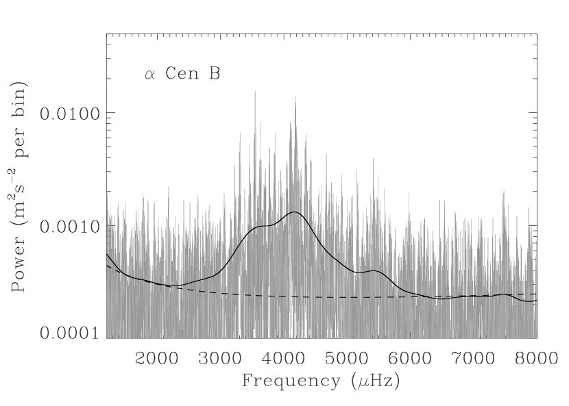
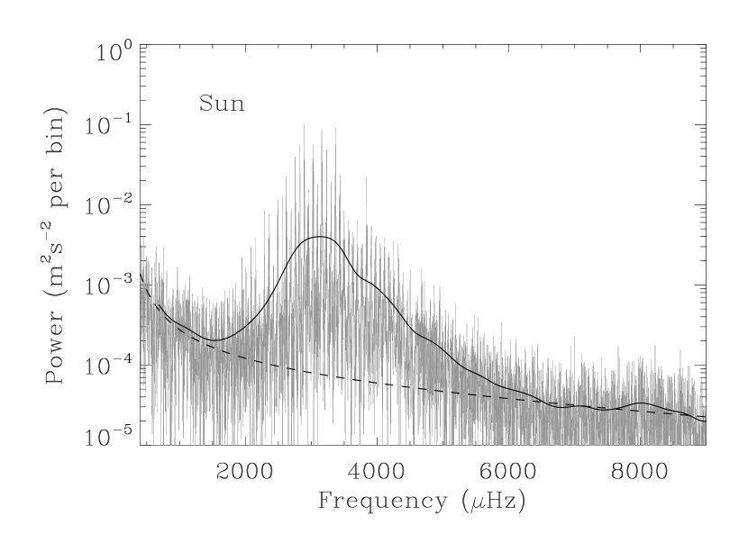
Figure 1: Left-hand panel: Observed frequency power spectrum of $\alpha$ Cen B (Kjeldsen et al. 2005). The dark solid line is the smoothed spectrum, while the dashed line is an estimate of the background. Right-hand panel: Observed frequency power spectrum of a 5-day segment of BiSON Sun-as-a-star data (linestyles as per left-hand panel).

The left-hand panel of Fig. 1 shows the observed frequency power spectrum of $\alpha$ Cen B, plotted on a logarithmic scale. The spectrum was computed from a few nights of Doppler velocity data collected by Kjeldsen et al. (2005). The dark solid line is a smoothed spectrum given by applying to the raw spectrum a Gaussian filter of width $4\Delta\nu$, where $\Delta\nu$ is the large frequency spacing between consecutive overtones (here $162\,\rm\mu Hz$). The dashed line is a smooth estimate of the background power spectral density. It was obtained by fitting, in regions outside the range occupied by the p modes, a second-order polynomial to the logarithm of power versus the logarithm of frequency.

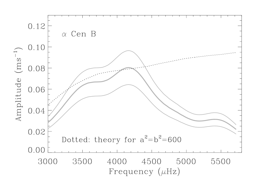
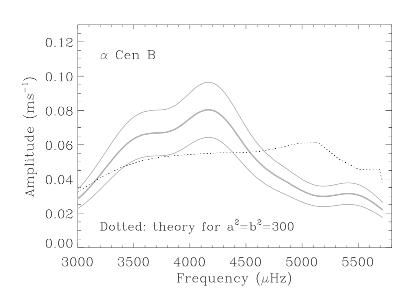
Figure 2: Observed mode velocity amplitudes $\rm V_{obs}$ (thick grey line) and theoretically computed amplitudes $V$ (dotted line) of $\alpha$ Cen B. The thin grey lines denote the estimated uncertainty envelope on the amplitudes (see text). Left-hand panel: theoretical predictions for $a^{2}=b^{2}=600$. Right-hand panel: theoretical predictions for $a^{2}=b^{2}=300$.

We used the Gaussian smoothed spectrum and the background fit to estimate the mode amplitudes, $V$. This was done by following the recipe outlined in Kjeldsen et al. (2008). In summary, we began by subtracting the background fit from the Gaussian-smoothed spectrum. The residuals thereby obtained were converted to units of power per Hertz, multiplied by the large frequency spacing $\Delta\nu$, and finally divided by a constant factor (see factors in Table 1 of Kjeldsen et al. 2008) to allow for the effective number of modes in each slice $\Delta\nu$ of the spectrum. This gave observational estimates of the radial mode amplitudes, $\rm V_{obs}$, which are plotted as a thick grey line in each panel of Fig. 2. The thin grey lines are an estimate of the uncertainty envelope on the observed amplitudes. These uncertainties were estimated by using as a guide the results of analyzing many independent, short segments of BiSON Sun-as-a-star data, as will be explained below.

We have used results on a parallel analysis of the BiSON Sun-as-a-star data as a belt-and-braces check on the procedures and results. The complete BiSON timeseries that we used is 4752 days long. This was split into independent segments of length 5 days (a length similar to the $\alpha$ Cen B timeseries), and the analysis procedures that were applied to the $\alpha$ Cen B frequency power spectrum were applied to the frequency power spectrum of each segment. The right-hand panel of Fig. 1 shows the frequency power spectrum of one of the 5-day BiSON segments (the layout and linestyles are the same as in the left-hand panel, and the spectrum was again smoothed over $4\Delta\nu$, but with $\Delta\nu=135\,\rm\mu Hz$ for the Sun).

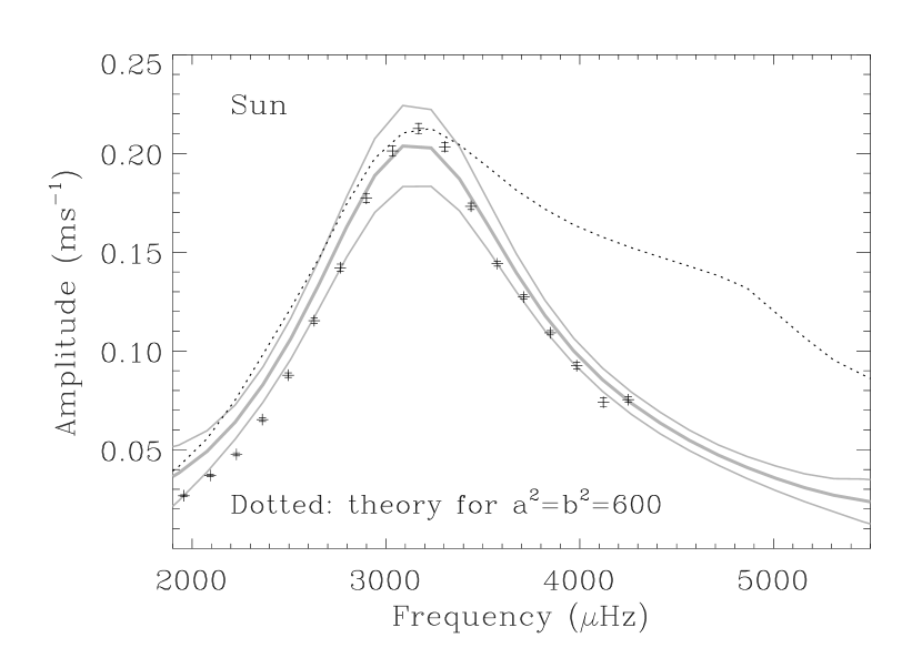
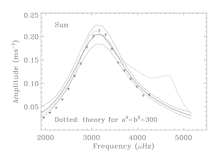
Figure 3: Observed mode velocity amplitudes $\rm V_{obs}$ (thick grey line) and theoretically computed amplitudes $V$ (dotted line) of the Sun. The plotted amplitudes are the mean amplitudes from analyzing 950 independent 5-day segments of BiSON Sun-as-a-star data. The thin grey lines denote the uncertainty envelope on the amplitudes, from the scatter in the results from the 5-day segments. The symbols with error bars are amplitudes $\rm V_{bag}$ given by a “peak-bagging” analysis of the full 4752-day BiSON timeseries. Left-hand panel: theoretical predictions for $a^{2}=b^{2}=600$. Right-hand panel: theoretical predictions for $a^{2}=b^{2}=300$.

The thick grey lines in both panels of Fig. 3 show the mean of the amplitudes that were obtained from the $\sim 950$ independent 5-day BiSON segments, using the method of Kjeldsen et al. outlined above. The thin grey lines mark plus and minus the rms of the amplitudes. Since the total epoch covered by the data spans more than one 11-yr cycle of solar activity, these uncertainties reflect variation of the estimated amplitudes from short-term stochastic variability and long-term solar cycle variability. There will also be a contribution from the finite signal-to-noise ratio of the observations.

The fractional uncertainties in the estimated 5-day BiSON amplitudes are about 15 % in the middle of the spectrum; and about 25 % at the extreme frequencies $\sim 2000$ and $\sim 5000\,\rm\mu Hz$, respectively. In the light of these values, we have assumed the estimated $\alpha$ Cen B amplitudes are all determined to a fractional precision of 20 %. This value was used to make the uncertainty envelope for the estimated $\alpha$ Cen B amplitudes plotted in both panels of Fig. 2.

With estimates of the uncertainties on $\rm V_{obs}$ now in hand, next we ask the question: how robust are the $\rm V_{obs}$ likely to be for $\alpha$ Cen B? We can obtain some insight by testing the robustness of the 5-day BiSON Sun-as-a-star amplitudes. This test may be accomplished by comparing the 5-day estimates with estimates from a “peak-bagging” analysis of the entire 4752-day BiSON timeseries. The BiSON mode amplitudes are usually estimated using the peak-bagging fitting techniques (e.g., see Chaplin et al. 2006). Peak-bagging involves maximum-likelihood fitting of mode peaks in the frequency power spectrum to multi-parameter fitting models, where individual mode peaks are represented by Lorentzian-like functions. The points with error bars in Fig. 3 show estimated amplitudes $\rm V_{bag}$ from a full peak-bagging analysis of the 4752-day BiSON timeseries, in which the mode peaks were fitted in the high-resolution frequency power spectrum of the complete timeseries. Since these peak-bagging estimates are extremely precise, and are also expected to be fairly accurate, they serve to provide a robust cross-check of the 5-day estimates. As we can see, the 5-day BiSON estimates are in good agreement with the peak-bagging BiSON estimates. This comparison suggests we may also expect to have reasonable confidence in the observed $\alpha$ Cen B amplitudes.

3.2 Comparison of theory with observation

Predictions from the pulsation computations of the p-mode velocity amplitudes, $V$, are shown as dotted lines in Fig. 2 ($\alpha$ Cen B) and Fig. 3 (Sun). The predicted amplitudes plotted in the left-hand panels of the figures are for $a^{2}=b^{2}=600$, while those in the right-hand panels are for $a^{2}=b^{2}=300$.

First, let us compare the modelled and observed amplitudes for $\alpha$ Cen B (Fig. 2). When $a^{2}=b^{2}=600$ (left-hand panel) the model amplitudes form a very broad plateau at frequencies $\gtrsim 3700\,\rm\mu Hz$, and the level of this plateau rises slowly with increasing frequency. While the match between the predicted amplitudes and the observed amplitudes is reasonable at frequencies $\lesssim 4500\,\rm\mu Hz$, this is demonstrably not so at higher frequencies, where the predicted amplitudes are significantly higher than the observed amplitudes. When $a^{2}=b^{2}=300$ the predicted amplitudes give a better match, on average, to the observed amplitudes, but some overestimation at higher frequencies remains.

High-frequency disagreement between theory and observation is also seen in Fig. 3 for the Sun. When $a^{2}=b^{2}=600$, we again see a pronounced disagreement at high frequencies between the predicted amplitudes and the observed amplitudes. When $a^{2}=b^{2}=300$ the level of disagreement is less pronounced, but is nevertheless still present.

Let us summarize the main points from Figs. 2 and 3: when $a^{2}=b^{2}=600$, theoretically computed high-frequency velocity amplitudes for $\alpha$ Cen B and the Sun significantly overestimate the observed velocity amplitudes. Although not as severe, this overestimation persists at $a^{2}=b^{2}=300$. What might be the cause of this disagreement between theory and observation? That is the question we turn to next.

4 Inference on the p-mode linewidths

Provided we trust the mode amplitudes $\rm V_{obs}$ estimated from the $\alpha$ Cen B frequency power spectrum – and the 5-day BiSON analysis above suggests the estimates should be reasonable – there are two possible ways out of the problem. Equation 2 implies that:

$$\frac{\delta V}{V}\sim\frac{\delta P}{2P}-\frac{\delta\eta}{2\eta}.$$ (4)

So, either the model damping rates $\eta$ – and therefore the model linewidths $\Delta$ – are too weak at high frequencies to explain the observed $\rm V_{obs}$, or the modelled acoustic supply rates, $P$, are too strong (or there is a combination of the two effects).

There is good evidence from analysis of Sun-as-a-star data (e.g., Chaplin et al. 2005; Houdek 2006) that a significant part of the disagreement may come from problems computing $\eta$ (and therefore $\Delta$). We can double-check the validity of this assumption here for the Sun, because we have precise BiSON data on the linewidths and powers of the solar p modes from the peak-bagging analysis. These peak-bagging data may be used as a precise and accurate reference against which to check the quality of the results obtained on the short 5-day BiSON segments.

4.1 The Sun-as-a-star linewidths

We base our solar check on Equation 2. Again, it tells us that $V^{2}\propto P/\Delta$. If we take the ratio of the observed to the model-computed velocity powers, we will therefore have:

$$\left(\frac{\rm V^{2}_{obs}}{V^{2}}\right)=\left(\frac{\rm P_{obs}}{P}\right)\left(\frac{\Delta}{\rm\Delta_{obs}}\right).$$ (5)

In the above, all observed quantities for the star, which we assume come from analysis of the short 5-day segments, carry the suffix “obs”; and the model-predicted quantities are suffix-free. Rearrangement of the above gives:

$${\rm\Delta_{obs}}=\left(\frac{\rm P_{obs}}{P}\right)\left(\frac{V^{2}}{\rm V^{2}_{obs}}\right)\Delta.$$ (6)

Let us suppose that all the problems in the modelling lie in computation of the linewidths, $\Delta$. The implication is then, of course, that the model-predicted values of the acoustic supply rates, $P$, are accurate, i.e., $P=\rm P_{obs}$. Equation 6 would then simplify to

$${\rm\Delta_{obs}}=\left(\frac{V^{2}}{\rm V^{2}_{obs}}\right)\Delta.$$ (7)

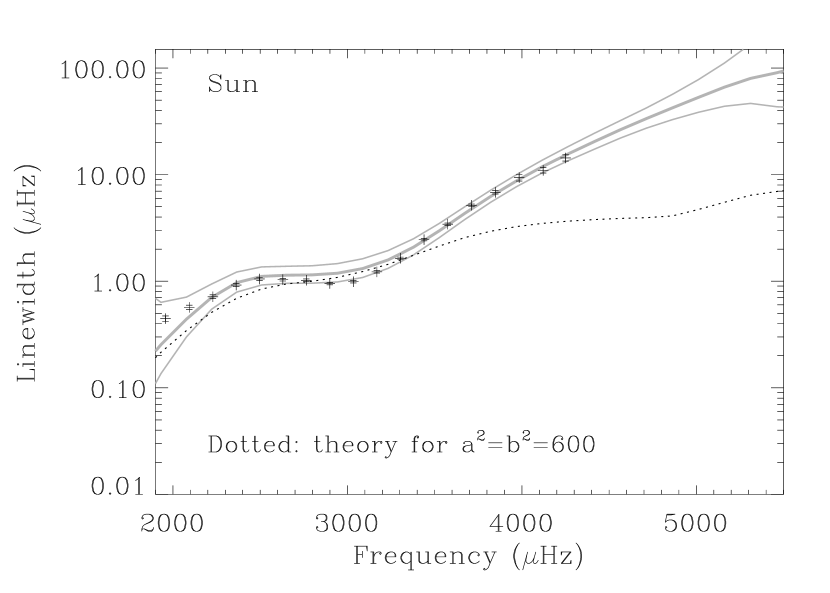
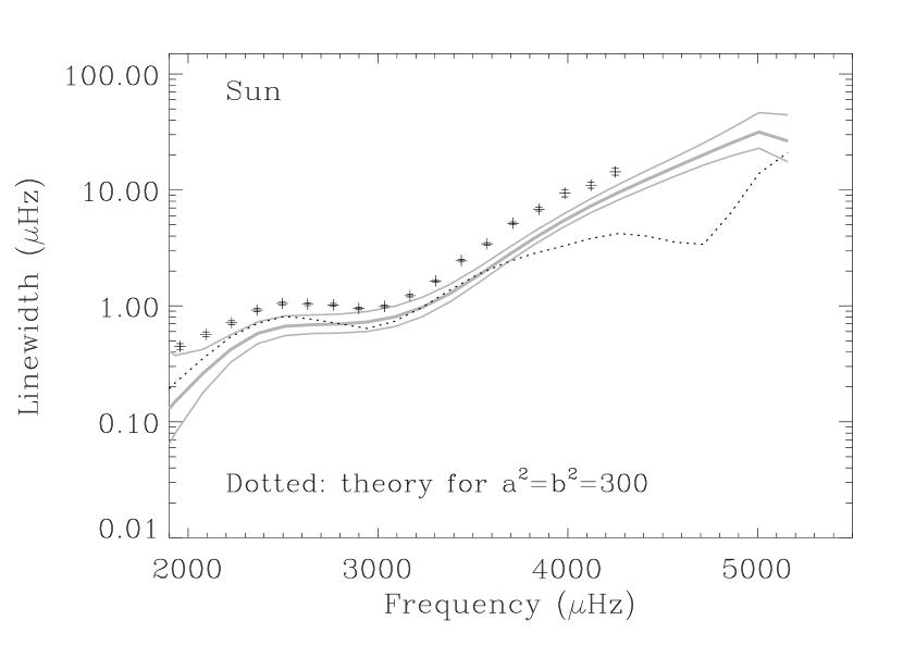
Figure 4: Inferred linewidths $\rm\Delta_{obs}$ (thick grey line) and theoretically computed linewidths $\Delta$ (dotted line) of the Sun. The theoretically computed linewidths have been smoothed with a median smoothing filter of three consecutive values, as in Houdek & Gough (2002). The plotted inferred linewidths are the mean inferred linewidths from analyzing 950 independent 5-day segments of BiSON Sun-as-a-star data. The thin grey lines denote the uncertainty envelope on the inferred linewidths, from the scatter in the results from the 5-day segments. The symbols with error bars are linewidths $\rm\Delta_{bag}$ given by a “peak-bagging” analysis of the full 4752-day BiSON timeseries. Left-hand panel: theoretical predictions for $a^{2}=b^{2}=600$. Right-hand panel: theoretical predictions for $a^{2}=b^{2}=300$.

How well do the solar model computations and 5-day observations match Equation 7, i.e., how well is the relation $P=\rm P_{obs}$ satisfied? Fig. 4 shows plots of the inferred linewidths $\rm\Delta_{obs}$ of the Sun (thick grey line). The $\rm\Delta_{obs}$ were computed from the observed 5-day $\rm V_{obs}$ in Section 3.1 above and the model predictions of $V^{2}$ and $\Delta$. The left-hand panel shows results for when the model computations use $a^{2}=b^{2}=600$; while the right-hand panel shows results with $a^{2}=b^{2}=300$. The thin grey lines show the uncertainty envelopes on the $\rm\Delta_{obs}$, which come from the uncertainties on $\rm V_{obs}$ shown in Fig. 3.

Also plotted as points with associated best-fitting uncertainties in Fig. 4 are the fitted linewidths $\rm\Delta_{bag}$ from a full 4752-day peak-bagging analysis of the BiSON Sun-as-a-star data. For our purposes here, we may regard the peak-bagging linewidths as being good measures of the true linewidths of the Sun. Our check on whether $P=\rm P_{obs}$ therefore amounts to seeing if the 5-day $\rm\Delta_{obs}$ are a good match to the $\rm\Delta_{bag}$. This does assume that there are no significant biases in the estimated $\rm V_{obs}$, as was suggested by the good agreement of the $\rm V_{obs}$ and $\rm V_{bag}$ in Fig. 3.

At a first glance, the most striking aspect of the solar plots is indeed the encouraging level of agreement between the $\rm\Delta_{obs}$ and the $\rm\Delta_{bag}$. Fig. 5 shows the comparison in more detail. Here, we have plotted the fractional differences between the 5-day linewidths and the peak-bagging linewidths. When $a^{2}=b^{2}=600$, the $\rm\Delta_{obs}$ over the main part of the solar p-mode spectrum are seen to be about 10 % higher on average than the $\rm\Delta_{bag}$, while they are about 35 % lower when $a^{2}=b^{2}=300$. The implication is that in both cases there is actually an offset between $P$ and $\rm P_{obs}$. However, what we can say is that changes in the differences as a function of frequency are not significant over the main part of the p-mode spectrum, given the observational uncertainties (we can disregard the differences at the lowest frequencies, where the error bars are very large, and the 5-day spectra have insufficient resolution to give robust estimates of $\rm\Delta_{obs}$ in this part of the spectrum). We are therefore in a position to conclude the following: the shape in frequency of the $\rm\Delta_{obs}$ is a reasonable match to the shape of the $\rm\Delta_{bag}$ at the level of precision of 5-day timeseries.

The above suggests we may use Equation 7 to infer the variation of the linewidths as a function of frequency, without the need to measure those linewidths directly. There will remain some uncertainty over the absolute calibration of the linewidths. Let us now apply Equation 7 to the data on $\alpha$ Cen B.

4.2 Inference on linewidths of $\alpha$ Cen B

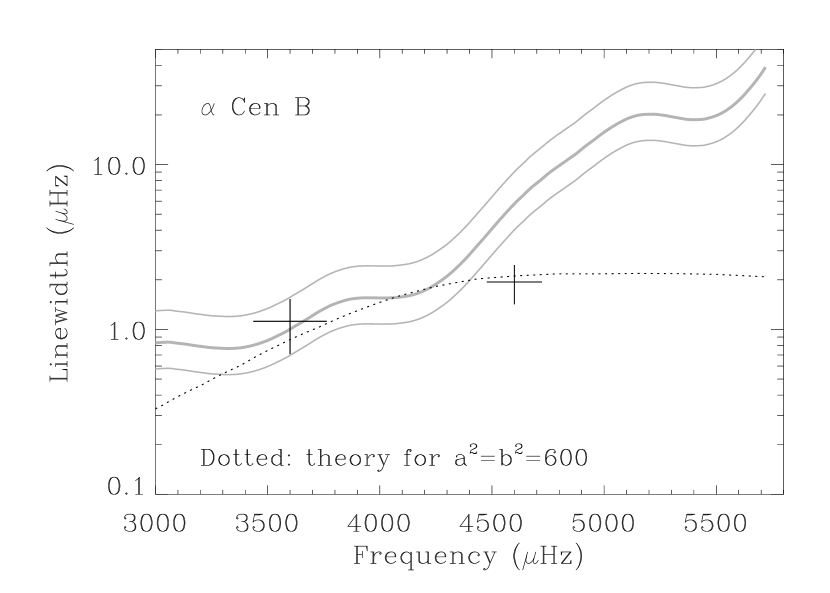
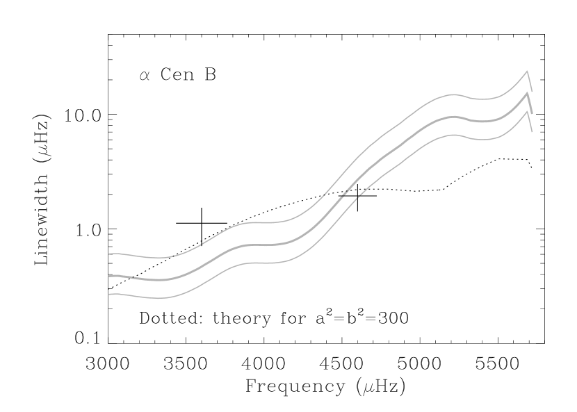
Figure 6: Inferred linewidths $\rm\Delta_{obs}$ (thick grey line) and theoretically computed linewidths $\Delta$ (dotted line) of $\alpha$ Cen B. The theoretically computed linewidths have been smoothed with a median smoothing filter of three consecutive values, as in Houdek & Gough (2002). The thin grey lines denote the estimated uncertainty envelope on the inferred linewidths (see text). The symbols with error bars show observational linewidth estimates from Kjeldsen et al. (2005). Left-hand panel: theoretical predictions for $a^{2}=b^{2}=600$. Right-hand panel: theoretical predictions for $a^{2}=b^{2}=300$.

We have used the observed estimates of $\rm V_{obs}$ from the $\alpha$ Cen B spectrum, together with the theoretical computations of $V$ and $\Delta$ for the star, to give the inferred linewidths $\rm\Delta_{obs}$ plotted in Fig. 6. We do not require an explicit estimate of $\rm P_{obs}$, because we rely on the assumption (verified above for the Sun) that the theoretical $P$ has the same shape in frequency as $\rm P_{obs}$.

There is no obvious reason why we should expect the acoustic supply-rate computations, $P$, to be any less valid for $\alpha$ Cen B than they are for the Sun (this might not have been so had $\alpha$ Cen B been somewhat hotter than the Sun, or much cooler than it actually is; see Houdek 2006). At the very least we may therefore have reasonable confidence in the shapes of the inferred linewidth curves for the star, assuming any deviations from a constant scaling offset are no more severe than they are for the Sun. Both curves in Fig. 6 appear to show a plateau in the linewidths at $4000\,\rm\mu Hz$, like that seen in the solar linewidth curve. Other obvious features of the curves – a decrease of the linewidths at lower frequencies, and an increase at higher frequencies – are also Sun-like in nature. It is worth stressing that the linewidth curves have very similar shapes at $a^{2}=b^{2}=600$ (left-hand panel) and $a^{2}=b^{2}=300$ (right-hand panel).

We have also shown on Fig. 6 observational linewidth estimates, which were obtained by Kjeldsen et al. (2005) in two parts of the p-mode spectrum (points with associated uncertainties). These estimates were obtained from the same data but in a different way, namely by measuring the scatter of p-mode frequencies around smooth ridges in the echelle diagram. Comparison of the inferred $\rm\Delta_{obs}$ with the Kjeldsen et al. estimates allows us to place constraints on the absolute values of the linewidths for $\alpha$ Cen B. Such a comparison suggests there is actually little to choose between the $\rm\Delta_{obs}$ and the Kjeldsen et al. estimates when the energy supply rates are computed using $a^{2}=b^{2}=600$ (giving the inferred linewidths in the left-hand panel of Fig. 6) or $a^{2}=b^{2}=300$ (giving the inferred linewidths in the right-hand panel). However, the $a^{2}=b^{2}=300$ result does give a slightly better match. Inspection of the $\rm\Delta_{obs}$ linewidth curve then implies that the $\alpha$ Cen B linewidths take values of about $0.4\,\rm\mu Hz$ at a frequency of $3500\,\rm\mu Hz$, about $0.8\,\rm\mu Hz$ at a frequency of $4000\,\rm\mu Hz$, and about $2.5\,\rm\mu Hz$ at a frequency of $4500\,\rm\mu Hz$. These linewidths turn out to agree reasonably well with the solar linewidths, if the mode frequencies are multiplied by the ratio of the acoustic cut-off frequencies of the two stars (which in effect scales the $\alpha$ Cen B frequencies down to those shown by the Sun). In short, the $\alpha$ Cen B linewidth curve is similar to a frequency-scaled version of its solar cousin.

5 Discussion

In this paper we presented an analysis of the amplitudes and linewidths of the low-degree, Sun-like p modes displayed by the star $\alpha$ Cen B. These data were extracted from only a few nights of Doppler velocity observations collected on the star by Kjeldsen et al. (2005), and were compared with theoretical predictions of the stochastic excitation and damping rates of the p modes. We also performed a parallel analysis of Sun-as-a-star p-mode data collected by the ground-based BiSON. The very long BiSON timeseries allowed us to validate the analysis techniques.

For the Sun, we found that model predictions of the mode amplitudes were significantly larger than the observed amplitudes in the high-frequency part of the p-mode spectrum. We were able to confirm that most of the disagreements for the Sun, which set in at frequencies $\gtrsim 3300\,\rm\mu Hz$, are due to problems computing the damping rates, not the excitation rates, of the modes. The computed damping rates must be increased to explain the observed amplitudes.

Similar disagreements are seen for $\alpha$ Cen B. Here, we do not have the luxury of cross-checking the analysis with results from very long datasets, since the latter at present do not exist [although we may hope to obtain such datasets in the future from the likes of SONG (Grundahl et al. 2007) and SIAMOIS (Mosser et al. 2007)]. However, by assuming that the disagreements for $\alpha$ Cen B are also due largely to problems with the model-predicted damping rates, as was shown to be the case for the Sun, we were able to demonstrate that the model linewidths must also be increased significantly in order to explain the observed amplitudes. The problems for $\alpha$ Cen B set in at frequencies $\gtrsim 4500\,\rm\mu Hz$.

The conclusions above bear on a prediction of the pulsation computations mentioned in the Introduction (Section 1): that stars cooler than about 5400 K will show a broad plateau or double-hump of power in their p-mode spectra. We showed that $\alpha$ Cen B does not have the predicted broad plateau in its observed p-mode spectrum. If the high-frequency damping rates are increased – as they must be to resolve the disagreement between theory and observation – the broad plateau or second high-frequency hump disappears in the cooler models.

Finally, we also showed how, by making suitable comparisons of theory and observation, it is possible to make inference on the variation with frequency of the p-mode linewidths without directly measuring those linewidths, even if the observations come from only a few days of data. Use of independent measures of the $\alpha$ Cen B linewidths, made in two parts of its spectrum by Kjeldsen et al. (2005), allowed us to calibrate our inferred linewidth curve for $\alpha$ Cen B. We found that the resulting, calibrated linewidth curve is similar to a frequency-scaled version of its solar cousin, with the scaling factor equal to the ratio of the respective acoustic cut-off frequencies of the two stars. The ratio of the frequencies at which the onset of high-frequency problems is seen in both stars is also given approximately by the same scaling factor.

Figure 5: Results on the solar p-mode linewidths. Plotted are differences in the natural logarithms (i.e., absolute fractional differences) of the inferred linewidths, $\rm\Delta_{obs}$ (which use data from the 5-day BiSON segments) and peak-bagging linewidths, $\rm\Delta_{bag}$ (from the frequency power spectrum of the full 4752-day BiSON timeseries).

References

- (1) Baker N., Kippenhahn R., 1965, ApJ, 142, 868
- (2) Balmforth N.J., 1992a, MNRAS, 255, 603
- (3) Balmforth N.J., 1992b, MNRAS, 255, 639
- (4) Chaplin W. J., et al., 1996, Sol Phys, 168, 1
- (5) Chaplin W. J., Houdek G., Elsworth Y., Gough D. O., New R., 2005, MNRAS, 360, 859
- (6) Chaplin W. J., et al., 2006, MNRAS, 369, 985
- (7) Chaplin W. J., Elsworth Y., Houdek G., New R., 2007, MNRAS, 377, 17
- (8) Chaplin W. J., Houdek G., Appourchaux T., Elsworth Y., New R., Toutain T., 2008, A&A, 485, 813
- (9) Christensen-Dalsgaard J., 1982, MNRAS, 199, 735
- (10) Eggleton P., Faulkner J., Flannery B.P., 1973, A&A, 23, 325
- (11) Fletcher S. T., Chaplin W. J., Elsworth Y., Schou J., Buzasi D., 2006, MNRAS, 371, 935
- (12) Goldreich P., Keeley D.A., 1977, ApJ 212, 243
- (13) Gough D.O., 1977a, in Spiegel E., Zahn J.-P., eds, Problems of stellar convection. Springer-Verlag, Berlin, p. 15
- (14) Gough D. O., 1977b, ApJ, 214, 196
- (15) Grundahl F., Kjeldsen H., Christensen-Dalsgaard J., Arentoft A., Frandsen S., 2007, CoAst, 150, 300
- (16) Houdek G., Balmforth N. J., Christensen-Dalsgaard J., Gough D. O., 1999, A&A, 351, 582
- (17) Houdek G., Gough D. O., 2002, MNRAS, 336, 65
- (18) Houdek G., 2006, in: Beyond the Spherical Sun, SOHO18/GONG 2006/HELAS I, eds. D. Dansey, M. J. Thompson, ESA SP-624, Sheffield, UK, p. 28.1
- (19) Iglesias C. A., Rogers F. J., 1996, ApJ, 464, 943
- (20) Kjeldsen H., Bedding T. R., Butler R. P., et al., 2005, ApJ, 635, 1281
- (21) Kjeldsen H., et al., 2008, ApJ, in press
- (22) Kolmogorov A.N., 1941, Dokl. Akad. Nauk SSSR, 30, 299
- (23) Kurucz R. L., 1991, in Crivellari L., Hubney I., Hummer D. G., eds, Stellar Atmospheres: Beyond Classical Models. Kluwer, Dordrecht, p. 441
- (24) Mosser B., and the SIAMOIS Team, 2007, in: 1st ARENA Conference on “Large Astronomical Infrastructures at CONCORDIA, prospects and constraints for Antarctic Optical/IR Astronomy”, eds. N. Epchtein, M. Candidi, EAS Publication Series 25, p. 239
- (25) Unno W., Spiegel E. A., 1966, PASJ, 18, 85
- (26) Yildiz M., 2007, MNRAS, 374, 1264