TWO-DIMENSIONAL STELLAR EVOLUTION CODE INCLUDING ARBITRARY MAGNETIC FIELDS. II. PRECISION IMPROVEMENT AND INCLUSION OF TURBULENCE AND ROTATION

Abstract

In the second paper of this series we pursue two objectives. First, in order to make the code more sensitive to small effects, we remove many approximations made in Paper I. Second, we include turbulence and rotation in the two-dimensional framework. The stellar equilibrium is described by means of a set of five differential equations, with the introduction of a new dependent variable, namely the perturbation to the radial gravity, that is found when the non-radial effects are considered in the solution of the Poisson equation; following the scheme of the first paper, we write the equations in such a way that the two-dimensional effects can be easily disentangled. The key concept introduced in this series is the equipotential surface. We use the underlying cause-effect relation to develop a recurrence relation to calculate the equipotential surface functions for uniform rotation, differential rotation, rotation-like toroidal magnetic fields and turbulence. We also develop a more precise code to numerically solve the two-dimensional stellar structure and evolution equations based on the equipotential surface calculations. We have shown that with this formulation we can achieve the precision required by observations by appropriately selecting the convergence criterion. Several examples are presented to show that the method works well. Since we are interested in modeling the effects of a dynamo-type field on the detailed envelope structure and global properties of the Sun, the code has been optimized for short timescales phenomena (down to 1 yr). The time dependence of the code has so far been tested exclusively to address such problems.

1 INTRODUCTION

High precision is an essential requirement in solar variability modeling because the cyclical variations of all solar global parameters are very small (see Li et al 2003 and references therein). For example, the (relative) precision of the measurements of the TSI is about $10^{-5}$. Oscillation splittings can also be measured with a similar precision, and the PICARD satellite expects to measure diameter changes with a precision of a few milli-arc seconds, thus a few parts in $10^{6}$. These requirements are even more extreme in the two-dimensional (2D) case, because two-dimensional effects are subtler than their 1D counterparts. This gives us a sense of the precision required for our code.

In the first paper of this series (Li et al 2006, referred hereafter as Paper I), we developed a 2D stellar evolution code that includes magnetic fields of arbitrary cylindrically symmetric configuration by generalizing in a straightforward way our one-dimensional (1D) code (Lydon & Sofia 1995; Li & Sofia 2001; Li et al 2002; Li et al 2003). Since the 2D case is very complex, we made some significant approximations, some physical, and some computational. In terms of the physical approximations, for the first two, we neglected the second-order derivative of the gravitational potential $\Phi$ with respect to the colatitude coordinate $\theta$ and the second-order derivative of the perturbation gravitational potential $\Phi-\Phi_{0}$ with respect to the radial coordinate $r$, where $\partial\Phi_{0}/\partial r=Gm/r^{2}$ is the spherically-symmetric gravitation acceleration component in the radial direction, i.e., expression (30) in Paper I. The third approximation is that we ignored turbulence, which had been included in our 1D variability models (Li et al 2002). A detailed comparison of the 1D solar variability models with the relevant observations (Li et al 2003) shows that turbulence must play an important role. In particular, in order to explain the changes of the oscillation spectrum in function of the activity cycle, we needed to include a model of turbulence that interacts with magnetic fields in a negative feedback sense. In this paper we remove these three physical approximations made in Paper I.

Unlike the three approximations mentioned above, the fourth approximation made in Paper I is computational, involving the solution method of the 2D stellar structure equations. In the 1D case, we use the trapezoidal rule to integrate the 1D stellar structure equations. In the 2D version in Paper I, the trapezoidal rule (or the central difference scheme) was not applied everywhere, since we used numerical derivatives. In this paper we minimize the use of numerical derivatives. The fifth approximation made in Paper I is that we neglected $\partial F_{\theta}/\partial\theta$ in the luminosity equation, i.e., the term $O(2)$ in Eq. (124d), which we now include. The similar term in Eq. (124e) of Paper I does not matter for the cyclic variation of the Sun.

Removal of the above six approximations is one of the main objectives of this paper. The second main objective is to include turbulence and rotation, which are also important sources for asphericity. In §2 we summarize the theoretical foundations that give rise to the 2D stellar variability models by including magnetic fields, turbulence and rotation. Since we want to get rid of approximations 1 and 2, we have to add the Poisson equation (which is a second-order partial differential equation) to the stellar structure equations. We thus have two more first-order stellar structure equations. As a result, we now have a total of six stellar structure equations.

Equipotential surface is the key concept to obtain the 2D generalization from the 1D stellar structure and evolution equations. In §3 we show how to find out the equipotential surface from the 2D stellar structure equations obtained in §2. Magnetic fields, turbulence and rotation are causes, and the resultant matter redistribution is the effect. This cause-effect relation indicates certain recurrence relation for equipotential surface calculations. We present the recurrence relations for the uniform rotation, differential rotations, rotation-like toroidal magnetic fields and turbulence in §3.

The third main objective of this paper is to raise the numerical precision of the numerical solutions for the 2D stellar structure and evolution equations. We tried hard to do so and found out that it is the best to explicitly invoke the equipotential surface. We present this method of solution in §4. We give a typical example of 2D solar variability models in §5 to show how we use this 2D code. The conclusion is presented in the last section.

2 THEORETICAL FOUNDATION

Magnetic fields, turbulence, and rotation are possible causes of asphericity. In this paper, we consider all of them. We assume that the system is azimuthally symmetric or axisymmetric. Therefore, we need only the radius ($r$) and colatitude ($\theta$) in the spherical polar coordinate ($r,\theta,\phi$), in which the azimuthal angle $\phi$ is irrelevant. The basic equations represent the conservation of mass, momentum, and energy. We also need the Poisson equation and the energy transport equation to close the system. Since magnetic fields are involved, the Maxwell equations must also be obeyed, for example, we require $\nabla\cdot{\bf B}=0$. In this section we summarize the results and point out the differences from their 1D counterpart.

2.1 Mass Conservation

Mass conservation is guaranteed by calculating the mass enclosed within a certain surface. In a spherically symmetric system the surface is a spherical surface with radius $r$ with respect to the symmetric center of the system. This spherical surface is also an equipotential surface of gravity. In the general case the equipotential surface $r=R(\Phi,\theta)$ is thus used to define the mass $M_{\Phi}$:

$$M_{\Phi}=2\pi\int_{0}^{\pi}d\theta\sin\theta\int_{0}^{R(\Phi,\theta)}drr^{2}\rho(r,\theta).$$ (1)

In the spherically symmetric case we have $M_{\Phi}=M_{r}$ since the equipotential surface $R(\Phi,\theta)$ and the density $\rho(r,\theta)$ do not depend upon colatitude $\theta$.

This mass expression sets up a one-to-one relationship between mass $M_{\Phi}$ and equipotential $\Phi$:

$$m\equiv M_{\Phi}=M_{\Phi}(\Phi),$$ (2)

which permits us to use mass $M_{\Phi}$ and colatitude $\theta$ as the 2D independent variables, instead of the gravitational potential $\Phi$ and colatitude $\theta$. Eq. (1) is the integral form of the mass conservation. Its differential form can be obtained by taking its partial derivative with respect to the equipotential surface $r=R(\Phi,\theta)$:

$$\frac{\partial m}{\partial r}=\frac{\partial M_{\Phi}}{\partial R}=4\pi r^{2}\rho_{m},$$ (3)

where

$$\rho_{m}\equiv\frac{1}{2r^{2}}\int_{0}^{\pi}d\theta R^{2}(\Phi,\theta)\rho(R(\Phi,\theta),\theta)\sin\theta.$$ (4)

This defines the density on the equipotential surface $r=R(\Phi,\theta)$. It should be pointed out that here $r$ is no longer a static Eulerian space coordinate, but a co-moving Lagrangian variable with an equipotential surface $\Phi=$ constant, as it is in the spherically symmetric case. Obviously, $\rho_{m}=\rho$ when the system is spherically symmetric. We use $r=r(m,\theta)$ to denote the functional relationship between $r$ and $m$.

Eq. (3) is our 2D mass conservation equation. Comparing it with its 1D counterpart,

$$\frac{\partial m}{\partial r}=4\pi r^{2}\rho,$$ (5)

we find that they differ by a correction factor $\rho_{m}/\rho$:

$$\frac{\partial m}{\partial r}=4\pi r^{2}\rho\left\{\frac{\rho_{m}}{\rho}\right\}.$$ (6)

This factor equals unity in the spherically symmetric case, but deviates from unity in the general case.

2.2 Momentum Conservation

When both turbulence and magnetic fields are taken into account, the momentum conservation of an equilibrium state can be expressed by the momentum equation

$$\nabla\cdot\left[\left(P+\frac{B^{2}}{8\pi}+\rho v^{\prime\prime}_{r}v^{\prime\prime}_{r}\right){\bf I}+\rho(v^{\prime\prime}_{\theta}v^{\prime\prime}_{\theta}-v^{\prime\prime}_{r}v^{\prime\prime}_{r})\hat{\bf e}_{\theta}\hat{\bf e}_{\theta}\right.$$

$$\left.+\rho(v^{\prime\prime}_{\phi}v^{\prime\prime}_{\phi}-v^{\prime\prime}_{r}v^{\prime\prime}_{r})\hat{\bf e}_{\phi}\hat{\bf e}_{\phi}-\frac{1}{4\pi}{\bf B}{\bf B}\right]=-\rho\nabla\Phi-\nabla\cdot(\rho{\bf v}{\bf v}),$$ (7)

where $P$ is the gas pressure, ${\bf B}$ is the magnetic field, ${\bf I}$ is the unit tensor with nonzero components $\hat{\bf e}_{r}\hat{\bf e}_{r}$, $\hat{\bf e}_{\theta}\hat{\bf e}_{\theta}$ and $\hat{\bf e}_{\phi}\hat{\bf e}_{\phi}$, and $v^{\prime\prime}_{i}$ is the turbulent velocity that is defined by the velocity variance:

$$v^{\prime\prime}_{i}=(\overline{v_{i}^{2}}-\overline{v_{i}}^{2})^{1/2},$$ (8)

where $i=r,\theta,\phi$. The over-bar denotes a combined horizontal and temporal average, and $v_{i}$ is the total velocity component. See Robinson et al (2003) for the details of 3D simulations to derive realistic turbulence properties in the solar convection zone, where $v^{\prime\prime}_{\theta}=v^{\prime\prime}_{\phi}$ is assumed. The regular motion velocity is denoted by ${\bf v}$, for example, ${\bf v}={\bf\Omega}\times{\bf r}$ for rotation, where ${\bf\Omega}$ is the rotation angular velocity.

For a system with magnetic fields, turbulence and rotation, Eq. (7) can be rewritten as follows:

$$\frac{\partial P_{T}}{\partial r} = -\rho\frac{\partial\Phi}{\partial r}+\rho({\cal H}_{r}+{\cal T}_{r}+{\cal R}_{r}),$$ (9)

$$\frac{1}{r}\frac{\partial P_{T}}{\partial\theta} = -\frac{\rho}{r}\frac{\partial\Phi}{\partial\theta}+\rho({\cal H}_{\theta}+{\cal T}_{\theta}+{\cal R}_{\theta}),$$ (10)

where the isotropic pressure components of the magnetic field ${\bf B}$, $P_{m}=B^{2}/8\pi$, and the radial pressure component of turbulence, $P_{t}=\rho v^{\prime\prime}_{r}v^{\prime\prime}_{r}$ have been added to the gas pressure, $P$, to define a total isotropic pressure $P_{T}=P+P_{m}+P_{t}$, while their anisotropic pressure components are denoted by ${\cal H}=\frac{1}{4\pi\rho}\nabla\cdot({\bf B}{\bf B})$ for the magnetic field ${\bf B}$, ${\cal T}=\rho^{-1}\nabla\cdot[\rho(v^{\prime\prime}_{r}v^{\prime\prime}_{r}-v^{\prime\prime}_{\theta}v^{\prime\prime}_{\theta})\hat{\bf e}_{\theta}\hat{\bf e}_{\theta}+\rho(v^{\prime\prime}_{r}v^{\prime\prime}_{r}-v^{\prime\prime}_{\phi}v^{\prime\prime}_{\phi})\hat{\bf e}_{\phi}\hat{\bf e}_{\phi}]$ for turbulence, and ${\cal R}=-\rho^{-1}\nabla\cdot(\rho{\bf v}{\bf v})$ for rotation, where ${\bf v}=\Omega\times{\bf r}$. Their $r$- and $\theta$-components are:

$$4\pi\rho{\cal H}_{r} = \frac{1}{r^{2}}\frac{\partial}{\partial r}(r^{2}B_{r}^{2})+\frac{1}{r}\frac{\partial}{\partial\theta}(B_{r}B_{\theta})-\frac{1}{r}(B_{\theta}^{2}+B_{\phi}^{2}),$$ (11a)

$$4\pi\rho{\cal H}_{\theta} = \frac{1}{r}\frac{\partial B_{\theta}^{2}}{\partial\theta}+\frac{1}{r}\frac{\partial}{\partial r}(rB_{r}B_{\theta})-\frac{B_{\phi}^{2}}{r}\cot\theta,$$ (11b)

$${\cal T}_{r} = \frac{2}{r}(v^{\prime\prime}_{\theta}v^{\prime\prime}_{\theta}-v^{\prime\prime}_{r}v^{\prime\prime}_{r}),$$ (11c)

$${\cal T}_{\theta} = -\rho^{-1}\frac{1}{r}\frac{\partial}{\partial\theta}[\rho(v^{\prime\prime}_{\theta}v^{\prime\prime}_{\theta}-v^{\prime\prime}_{r}v^{\prime\prime}_{r})],$$ (11d)

$${\cal R}_{r} = \Omega^{2}r\sin^{2}\theta,$$ (11e)

$${\cal R}_{\theta} = \Omega^{2}r\sin\theta\cos\theta.$$ (11f)

2.3 Poisson Equation

The Poisson equation in the spherical coordinate system with the specified symmetry requirement can be written down as follows :

$$\frac{1}{r^{2}}\frac{\partial}{\partial r}\left(r^{2}\frac{\partial\Phi}{\partial r}\right)+\frac{1}{r^{2}\sin\theta}\frac{\partial}{\partial\theta}\left(\sin\theta\frac{\partial\Phi}{\partial\theta}\right)=4\pi G\rho.$$ (12)

Solving this equation for the gravitational potential $\Phi$ is not sufficiently accurate for our purposes, especially in the core of stars. Solving it for the radial gravitational acceleration $g=\partial\Phi/\partial r$ is equally not good for the same reason. Many tries show that the following treatment is sufficiently accurate for our high-precision requirement.

First of all, we calculate the colatitudinal gravitational acceleration ${\cal G}\equiv(1/r)\partial\Phi/\partial\theta$ by using the hydrostatic equilibrium equation in the colatitudinal direction (Eq. 10) in terms of $\partial P_{T}/\partial\theta$, ${\cal H}_{\theta}$, and ${\cal T}_{\theta}$:

$${\cal G}={\cal H}_{\theta}+{\cal T}_{\theta}+{\cal R}_{\theta}-\frac{1}{r\rho}\frac{\partial P_{T}}{\partial\theta}.$$ (13)

This way, Eq. (10) is satisfied automatically. We then decompose $g$ into two parts,

$$g=\frac{Gm}{r^{2}}+\delta g.$$ (14)

The first part is the spherically-symmetric radial component of the gravitational acceleration, and the second part is the deviation of the radial gravitational acceleration from its spherically-symmetric counterpart. Substituting Eq. (14) into Eq. (12), we obtain

$$\frac{\partial\delta g}{\partial r}=4\pi G(\rho-\rho_{m})-\frac{2}{r}\delta g-\frac{{\cal G}\cot\theta}{r}-\frac{1}{r}\frac{\partial{\cal G}}{\partial\theta}.$$ (15)

Therefore, we solve the Poisson equation for $\delta g$ instead of $\Phi$ or $g$. Here we have used the notations $r^{\prime}=\ln r$, and $\rho^{\prime}=\ln\rho$. The hydrostatic equilibrium equation in the radial direction thus becomes:

$$\frac{\partial P_{T}}{\partial r}=-\rho\left(\frac{Gm}{r^{2}}+\delta g-{\cal H}_{r}-{\cal T}_{r}-{\cal R}_{r}\right).$$ (16)

2.4 Energy Conservation

The energy conservation equation is

$$\frac{1}{r^{2}}\frac{\partial}{\partial r}(r^{2}F_{r})+\frac{1}{r\sin\theta}\frac{\partial}{\partial\theta}(\sin\theta F_{\theta})=\rho\left(\epsilon-T\frac{dS_{T}}{dt}\right),$$ (17)

where ${\bf F}={\bf F}_{\mbox{\scriptsize{rad}}}+{\bf F}_{\mbox{\scriptsize{conv}}}$ is the energy flux vector, including both the radiative flux ${\bf F}_{\mbox{\scriptsize{rad}}}$ and the convective flux ${\bf F}_{\mbox{\scriptsize{conv}}}$, and $\epsilon$ is the rate of nuclear energy generation, and $S_{T}$ is the total specific entropy, including the contributions from magnetic fields and turbulence. We use the diffusion approximation for radiative flux, and the mixing length theory for convective flux:

$${\bf F}_{\mbox{\scriptsize{rad}}} = -\frac{4acT^{3}}{3\kappa\rho}\nabla T,$$ (18)

$${\bf F}_{\mbox{\scriptsize{conv}}} = -\frac{1}{2}\frac{\rho Tl_{m}v_{\mbox{\scriptsize{conv}}}}{1+v_{\mbox{\scriptsize{conv}}}/v_{0}}\nabla S_{T},$$ (19)

where $v_{\mbox{\scriptsize{conv}}}$ is the convection velocity, $l_{m}$ is the mixing length, $v_{0}$ is a typical velocity determined by choice of radiative loss mechanism of a convective eddy. The symbol $a$ represents the radiation constant, $c$ the speed of light, $\kappa$ the mass opacity coefficient. The 2D energy conservation equation shows that energy can not only penetrate a region via the radial gradient of the radial component of the energy flux, but also goes around it via the transverse gradient of the transverse component of the energy flux. In contrast, the 1D energy conservation equation

$$\frac{1}{r^{2}}\frac{d}{dr}(r^{2}F_{r})=\rho\left(\epsilon-T\frac{dS_{T}}{dt}\right)$$ (20)

rules out the transverse transport of energy.

2.5 Energy Transport

Eqs. (17-20) show that we have to calculate temperature and entropy gradients. We thus need the first law of thermodynamics in the presence of magnetic fields and turbulence. We have redefined the mechanical variable $P_{T}$ by adding all isotropic pressure components together. We need magnetic and turbulent variables to take into account magnetic and turbulent degrees of freedom.

2.5.1 Magnetic and turbulent variables

We use ${\bf B}$ to define three stellar magnetic parameters, in addition to the conventional stellar parameters such as pressure, temperature, radius and luminosity. The first magnetic parameter is the magnetic kinetic energy per unit mass, $\chi_{m}$,

$$\chi_{m}=B^{2}/(8\pi\rho).$$ (21)

The second is the heat index due to the magnetic field, or the ratio of the magnetic pressure in the radial direction to the magnetic energy density, $\gamma_{m}-1$,

$$\gamma_{m}=1+(B_{\theta}^{2}+B_{\phi}^{2})/B^{2}.$$ (22)

The third one is the ratio of the magnetic pressure in the colatitude direction to the magnetic energy density, $\vartheta_{m}-1$,

$$\vartheta_{m}=1+(B_{\phi}^{2}+B_{r}^{2})/B^{2}.$$ (23)

We can use these three magnetic parameters to express three components of a magnetic field as follows:

$$B_{r} = [8\pi(2-\gamma_{m})\chi_{m}\rho]^{1/2},$$ (24a)

$$B_{\theta} = [8\pi(2-\vartheta_{m})\chi_{m}\rho]^{1/2},$$ (24b)

$$B_{\phi} = [8\pi(\gamma_{m}+\vartheta_{m}-3)\chi_{m}\rho]^{1/2}.$$ (24c)

However, since $v^{\prime\prime}_{\theta}=v^{\prime\prime}_{\phi}$ is assumed, we have only two turbulent degrees of freedom and we thus need two turbulent variables, namely, the turbulent kinetic energy per unit mass, $\chi_{t}$, and the effective ratio of specific heats due to turbulence, $\gamma_{t}$:

$$\chi_{t}=\frac{1}{2}(v^{\prime\prime})^{2}, \gamma_{t}=1+2(v^{\prime\prime}_{r}/v^{\prime\prime})^{2}.$$ (25)

We can use them to express three turbulent velocity components:

$$v^{\prime\prime}_{r} = [(\gamma_{t}-1)\chi_{t}]^{1/2},$$ (26a)

$$v^{\prime\prime}_{\theta} = v^{\prime\prime}_{\phi}=\left[\frac{1}{2}(3-\gamma_{t})\chi_{t}\right]^{1/2}.$$ (26b)

2.5.2 Equation of state

Using the magnetic and turbulent variables defined above, we can rewrite the total pressure as follows:

$$P_{T}=P(\rho,T)+\rho\chi_{m}+\rho(\gamma_{t}-1)\chi_{t}.$$ (27)

Solving this equation for $\rho$, we obtain the equation of state in the presence of magnetic fields and turbulence:

$$\rho=\rho(P_{T},T,\chi_{m},\chi_{t},\gamma_{t}).$$ (28)

To highlight magnetic and turbulence effects we adopt a given chemical composition. This shows that the independent thermodynamical variables are $P_{T}$, $T$, $\chi_{m}$, $\chi_{t}$, and $\gamma_{t}$. Using them,we can write the differential form of the equation of state as follows:

$$d\rho/\rho=\alpha dP_{T}/P_{T}-\delta dT/T-\nu_{m}d\chi_{m}/\chi_{m}-\nu_{t}d\chi_{t}/\chi_{t}-\mu_{t}d\gamma_{t}/\gamma_{t},$$ (29)

where

$$\alpha\equiv(\partial\ln\rho/\partial\ln P_{T})_{T,\chi_{m},\chi_{t},\gamma_{t}},\hskip 14.22636pt\delta\equiv-(\partial\ln\rho/\partial\ln T)_{P_{T},\chi_{m},\chi_{t},\gamma_{t}},$$ (30a)

$$\nu_{m}\equiv-(\partial\ln\rho/\partial\ln\chi_{m})_{P_{T},T,\chi_{t},\gamma_{t}},\hskip 14.22636pt\nu_{t}\equiv-(\partial\ln\rho/\partial\ln\chi_{t})_{P_{T},T,\chi_{m},\gamma_{t}}$$ (30b)

$$\mu_{t}\equiv-(\partial\ln\rho/\partial\ln\gamma_{t})_{P_{T},T,\chi_{m},\chi_{t}}.$$ (30c)

When a $\theta$-dependent magnetic field is applied, Eq. (28) demonstrates that the mass distribution will adjust to generate asphericity. This is the most straightforward 2D effect.

2.5.3 The first law of thermodynamics in the presence of magnetic fields and turbulence

The first law of thermodynamics is the energy transfer and conservation law in a thermodynamic system. In the presence of magnetic fields and turbulence, the conservation law should be modified as follows:

$$TdS_{T}=dU+PdV-d\chi_{m}-d\chi_{t},$$ (31)

which states that both magnetic and turbulent energy are generated at the expense of internal energy of the system $U$. Here $V=1/\rho$ is the specific volume. Combining Eqs. (28) and (31) (see Lydon & Sofia 1995 for the detail), we obtain

$$TdS_{T}=C_{p}dT-\left(\frac{\delta}{\rho}\right)dP_{T}+\left(\frac{P_{T}\delta\nu_{m}}{\alpha\rho\chi_{m}}-1\right)d\chi_{m}+\left(\frac{P_{T}\delta\nu_{t}}{\alpha\rho\chi_{t}}-1\right)d\chi_{t}+\frac{P_{T}\delta\mu_{t}}{\alpha\rho\gamma_{t}}d\gamma_{t},$$ (32)

from which we obtain

$$\nabla S_{T} = (C_{p}/T)\nabla T-(C_{p}\nabla^{\prime}_{\mbox{\scriptsize{ad}}}/P_{T})\nabla P_{T},$$ (33)

$$\frac{dS_{T}}{dt} = (C_{p}/T)\frac{dT}{dt}-(C_{p}\nabla^{\prime}_{\mbox{\scriptsize{ad}}}/P_{T})\frac{dP_{T}}{dt}.$$ (34)

We have defined the modified adiabatic gradient

$$\nabla^{\prime}_{\mbox{\scriptsize{ad}}}=\nabla_{\mbox{\scriptsize{ad}}}\left[1-\left(\frac{\nu_{m}}{\alpha}-\frac{\chi_{m}}{C_{p}T}\right)\nabla_{m}-\left(\frac{\nu_{t}}{\alpha}-\frac{\chi_{t}}{C_{p}T}\right)\nabla_{t}-\frac{\mu}{\alpha}\nabla_{\gamma}\right],$$ (35)

where $C_{p}$ is the specific heat per unit mass at constant total pressure, constant magnetic energy per unit mass, constant turbulent kinetic energy per unit mass, and constant turbulent specific heat ratio, and

$$\nabla_{\mbox{\scriptsize{ad}}}=P_{T}\delta/(\rho C_{p}T),\hskip 8.53581pt\nabla_{m}=\frac{\partial\ln\chi_{m}}{\partial\ln P_{T}},\hskip 8.53581pt\nabla_{t}=\frac{\partial\ln\chi_{t}}{\partial\ln P_{T}},\hskip 8.53581pt\nabla_{\gamma}=\frac{\partial\ln\gamma_{t}}{\partial\ln P_{T}}.$$

The physical meaning of Eq. (35) is that magnetic fields and turbulence provide additional channels for energy transport.

2.5.4 Energy flux vector

Using Eqs. (18-19) and (33) the energy flux vector ${\bf F}$ can be expressed by the temperature gradient $\nabla T$ and pressure gradient $\nabla P_{T}$ as follows:

$${\bf F} = -\left(\frac{4acT^{3}}{3\kappa\rho}+\frac{1}{2}\frac{\rho C_{P}l_{m}v_{\mbox{\scriptsize{conv}}}}{1+v_{\mbox{\scriptsize{conv}}}/v_{0}}\right)\nabla T$$ (36)

$$+\frac{1}{2}\frac{\rho C_{P}T\nabla^{\prime}_{\mbox{\scriptsize{ad}}}l_{m}v_{\mbox{\scriptsize{conv}}}}{1+v_{\mbox{\scriptsize{conv}}}/v_{0}}\frac{1}{P_{T}}\nabla P_{T}.$$

Its $r$-component determines the radial temperature gradient, its $\theta$-component results in 2D effect.

3 EQUIPOTENTIAL SURFACE

Solar magnetic fields are weak in the sense that the resultant magnetic pressure is much smaller than the gas pressure. The usual central difference scheme alone may not discern the required 2D effects. We should therefore use certain physical guidelines to improve the precision of the numerical solutions for the 2D stellar structure equations. The key concept introduced for the 2D stellar structure in this series is the equipotential surface. In this section we show how to determine it.

3.1 Exact 2D Stellar Structure Equations

The exact 2D stellar structure equations, i.e., Eqs. (6), (13), (15), (16), (17), and the energy transport equation, can be rewritten as follows after coordinate transformation from $(r,\theta)$ to $(m,\theta)$:

$$\frac{\partial r^{\prime}}{\partial s} = \frac{m}{4\pi r^{3}\rho}\frac{\rho}{\rho_{m}},$$ (37a)

$$\frac{\partial P^{\prime}}{\partial s} = -\frac{m}{4\pi r^{2}P_{T}}\frac{\rho}{\rho_{m}}\left(\frac{Gm}{r^{2}}+U-{\cal H}_{r}-{\cal T}_{r}-{\cal R}_{r}\right),$$ (37b)

$$\frac{\partial T^{\prime}}{\partial s} = \frac{\partial P^{\prime}}{\partial s}\left\{\begin{array}[]{ll}\nabla_{\mbox{\scriptsize{rad}}}&\mbox{ radiative}\\ \nabla_{\mbox{\scriptsize{c}}}&\mbox{ convective}\\ \end{array}\right.$$ (37e)

$$\frac{\partial L}{\partial s} = \frac{1}{L_{\sun}}m\left(\epsilon-T\frac{dS_{T}}{dt}\right)\frac{\rho}{\rho_{m}}-\frac{1}{L_{\sun}}\frac{mF_{\theta}\cot\theta}{r\rho_{m}}-\frac{1}{L_{\sun}}\frac{m}{r\rho_{m}}\frac{\partial F_{\theta}}{\partial\theta},$$ (37f)

$$\frac{\partial U}{\partial s} = \frac{Gm}{r^{2}}\left(\frac{\rho}{\rho_{m}}-1\right)-\frac{m}{4\pi r^{3}\rho_{m}}\left(2U+{\cal G}\cot\theta+\frac{\partial{\cal G}}{\partial\theta}\right).$$ (37g)

Here $P^{\prime}=\ln P_{T}$, $T^{\prime}=\ln T$, $r^{\prime}=\ln r$, $L=4\pi r^{2}F_{r}/L_{\sun}$, and $U=\delta g$. The other symbols used above are defined as follows:

$$F_{\theta} = \left\{-\left[\frac{4acT^{4}}{3\kappa\rho}+\frac{1}{2}\frac{\rho C_{P}Tl_{m}v_{\mbox{\scriptsize{conv}}}}{1+v_{\mbox{\scriptsize{conv}}}/v_{0}}\right]\frac{\nabla}{r}+\frac{1}{2}\frac{\rho C_{P}Tl_{m}v_{\mbox{\scriptsize{conv}}}}{1+v_{\mbox{\scriptsize{conv}}}/v_{0}}\frac{\nabla^{\prime}_{\mbox{\scriptsize{ad}}}}{r}\right\}\frac{\partial P^{\prime}}{\partial\theta},$$ (38a)

$${\cal G} = {\cal H}_{\theta}+{\cal T}_{\theta}+{\cal R}_{\theta}-\frac{P_{T}}{r\rho}\frac{\partial P^{\prime}}{\partial\theta}.$$ (38b)

These equations show that in addition to the dependent variables, pressure $P_{T}$, temperature $T$, radius $r$, and luminosity $L$, we have two more dependent variables, the radial and colatitudinal gravitational acceleration perturbations $\delta g$ and ${\cal G}$. However, we need to solve only five partial differential equations (Eqs. 37a-37g) because the colatitudinal gravitational acceleration ${\cal G}$ can be calculated by using $\left(\frac{\partial P_{T}}{\partial\theta}\right)_{m}$, $\left(\frac{\partial r^{\prime}}{\partial\theta}\right)_{m}$, ${\cal H}_{\theta}$, ${\cal T}_{\theta}$, and ${\cal R}_{\theta}$.

We use $\delta g=0$ at $m=0$ as the central boundary condition for the fifth equation because $\delta g$ is a perturbation in nature. This is equivalent to assume that the radial gravitational acceleration be equal to its spherically symmetric counterpart at the center.

3.2 Equipotential Surface Profile

We know that $r$ is the radial coordinate of an equipotential surface. Its dependence on the colatitudinal coordinate $\theta$, i.e., $r=r(\Phi,\theta)=r(m,\theta)$ defines an equipotential surface on which the potential equals $\Phi$. We redefine $r$ by $r_{e}=r_{e}(m)$ and $x=x(m,\theta)$: $r=r_{e}(m)x(m,\theta)$, where $r_{e}$ is the equatorial radius. Since we interpret $r_{e}$ as the equatorial radius, $x$ should always be normalized so that we obtain $x=1$ at the equator where $\theta=\pi/2$. The equipotential surface is thus expressed by $x=x(m,\theta)$, which is a function of mass $m=M_{\Phi}(\Phi)$ and colatitude $\theta$.

In order to find out the equipotential surface $x$, we use the fact that pressure is $\theta$-independent on it. Otherwise, the hydrostatic equilibrium is not reached thereon. This indicates that $\frac{\partial P_{T}}{\partial s}$ should be $\theta$-independent thereon as well. The following equation is $\theta$-independent and holds well for both spherically-symmetric and aspherical cases:

$$\frac{\partial P^{\prime}}{\partial s}=-\frac{Gm^{2}}{4\pi r_{e}^{4}P_{T}}.$$ (39)

Comparing it with Eq. (37b), we obtain

$$x^{4}=\frac{\rho}{\rho_{m}}\left[1+\frac{r_{e}^{2}x^{2}}{Gm}\left(U-{\cal H}_{r}-{\cal T}_{r}-{\cal R}_{r}\right)\right].$$ (40)

We can use the iteration method to obtain $x$ starting from $x=1$ if we know $r_{e}$, $U$, ${\cal H}_{r}$, ${\cal T}_{r}$, and ${\cal R}_{r}$. Eq. (4) that is used to determine $\rho/\rho_{m}$ now becomes

$$\rho_{m}=\frac{1}{x^{2}}\int_{0}^{\pi/2}\rho x^{2}\sin\theta d\theta.$$ (41)

3.2.1 Mass conservation for $r_{e}$

To calculate $r_{e}$, we rewrite the mass conservation equation as follows:

$$\frac{\partial r}{\partial m}=1/Q,$$ (42)

where

$$Q\equiv 4\pi r^{2}\rho_{m}$$ (43)

is $\theta$-independent. As a result, we know that $\frac{\partial r}{\partial m}$ is $\theta$-independent. Therefore, we can choose $r$ at any specific colatitude on the equipotential surface. We can, of course, choose $r=r_{e}(m)$ to obtain

$$\frac{\partial r_{e}^{\prime}}{\partial s}=\frac{m}{Qr_{e}},$$ (44)

where $r^{\prime}_{e}\equiv\ln r_{e}$.

Eq. (44) becomes

$$m=\frac{1}{3}Qr_{e}$$ (45)

at the center. This is one of the central boundary conditions.

3.2.2 Poisson equation for $U$

The radial gravitational acceleration perturbation $U=\delta g$ can be decomposed into five components $U=U_{D}+U_{P}+U_{H}+U_{T}+U_{R}$ according to their physical origins specified by the subscripts, where subscript D stands for the density variation, P for the pressure variation, H for magnetic fields, T for turbulence, and R for rotation. To see this, we decompose the colatitudinal gravitational acceleration component into four components according to their physical ingredients ${\cal G}={\cal G}_{P}+{\cal G}_{H}+{\cal G}_{T}+{\cal G}_{R}$. Their definitions are

$${\cal G}_{P} = -\frac{GmQ}{4\pi r_{e}^{4}\rho}\left(\frac{\partial x^{\prime}}{\partial\theta}\right)_{m},$$ (46a)

$${\cal G}_{H} = {\cal H}_{\theta},$$ (46b)

$${\cal G}_{T} = {\cal T}_{\theta},$$ (46c)

$${\cal G}_{R} = {\cal R}_{\theta},$$ (46d)

where we have utilized the equipotential surface condition $\left(\frac{\partial P^{\prime}}{\partial\theta}\right)_{m}=0$ and defined $x^{\prime}\equiv\ln x$. Since the Poisson equation is linear, we can write it down for each component as follows:

$$\frac{\partial U_{i}}{\partial r}=-\frac{2U_{i}}{r}+S_{i},$$ (47)

where i = D, P, H, T, and R. The source terms $S_{i}$ are expressed by the following functions:

$$S_{D} = 4\pi G(\rho-\rho_{m}),$$ (48a)

$$S_{i} = -\frac{{\cal G}_{i}\cot\theta}{r}-\frac{1}{r}\frac{\partial{\cal G}_{i}}{\partial\theta},$$ (48b)

where i = P, H, T, and R. Eq. (47) has a specific solution:

$$U_{i}=\frac{1}{x^{2}}\int_{0}^{r}x^{2}S_{i}dr.$$ (49)

3.3 Uniform Rotation Rate

3.3.1 Uniform rotation equipotential surface

We want to use this special case to show how to obtain the equipotential surface $x=x(m,\theta)$.

For rotation at the angular velocity $\Omega\hat{z}$, we can use Eq. (49) to calculate the radial gravitational acceleration perturbation $U_{R}$. The result is

$${\cal G}_{R} = {\cal R}_{\theta}=\frac{1}{2}\Omega^{2}r\sin 2\theta,$$

$$S_{R} = -\frac{3}{2}\Omega^{2}(\cos 2\theta+\frac{1}{3}),$$

$$U_{R} = -\frac{3}{2}\Omega^{2}r(\cos 2\theta+\frac{1}{3}).$$

Here we assume that $\Omega=\Omega(r)$ does not depend upon $\theta$. Eq. (40) shows that we need

$$U_{R}-{\cal R}_{r}=-\Omega^{2}r(\cos 2\theta+1).$$

As the first approximation, we assume $\rho/\rho_{m}=1$, $x=1$, and $U_{P}=U_{D}=0$ in Eq. (40). For a slow rotation in the sense that the centrifugal acceleration $\Omega^{2}r_{e}$ is much smaller than the corresponding gravitational acceleration $Gm/r_{e}^{2}$, we obtain

$$x^{(0)}=1-\frac{1}{4}a_{0}(\cos 2\theta+1),$$ (50)

where

$$a_{0}=\frac{\Omega^{2}r^{3}}{Gm}.$$

We can further improve the result by taking into account $\varpi\equiv\rho/\rho_{m}$, $\Lambda\equiv\left(\frac{\partial x^{\prime}}{\partial\theta}\right)_{m}$, $U_{P}$, and $U_{D}$ in Eq. (40):

$$\varpi^{(0)} = 1-\frac{1}{2}a_{0}(\cos 2\theta+\frac{1}{3}),$$

$$\Lambda^{(0)} = \frac{1}{2}a_{0}\sin 2\theta,$$

$${\cal G}_{P}^{(0)} = -\frac{1}{2}\frac{Gma_{0}}{r^{2}}\sin 2\theta,$$

$$S_{P}^{(0)} = \frac{1}{2}(\cos 2\theta+\frac{1}{3})\frac{3Gma_{0}}{r^{3}},$$

$$S_{D}^{(0)} = -\frac{1}{2}(\cos 2\theta+\frac{1}{3})4\pi Ga_{0}\rho,$$

$$U_{P}^{(0)} = \frac{1}{2}(\cos 2\theta+\frac{1}{3})b_{P}^{(0)},$$

$$U_{D}^{(0)} = -\frac{1}{2}(\cos 2\theta+\frac{1}{3})b_{D}^{(0)},$$

where

$$b_{P}^{(0)}=3\int_{0}^{r}\frac{Gma_{0}}{r^{3}}dr,\hskip 8.53581ptb_{D}^{(0)}=4\pi G\int_{0}^{r}a_{0}\rho dr.$$

The corrected equipotential surface function is

$$x^{(1)}=1+\frac{1}{12}[a_{0}+\frac{r^{2}}{Gm}(b_{D}^{(0)}-b_{P}^{(0)})]-\frac{1}{4}a_{1}(\cos 2\theta+1),$$ (51)

where

$$a_{1}=a_{0}+a_{0}^{\prime},\hskip 8.53581pta_{0}^{\prime}=\frac{1}{2}[a_{0}+\frac{r^{2}}{Gm}(b_{D}^{(0)}-b_{P}^{(0)})].$$

According to the definition of $x$, it should equal unity at the equator. This requirement fixes the expression of $x$ as follows:

$$x^{(1)}=1-\frac{1}{4}a_{1}(\cos 2\theta+1).$$ (52)

From now on, we shall show this form only, which will be referred to as the normalized form.

Using Eq. (52) or its non-normalized form we can improve $\varpi$, $\Lambda$, $U_{P}$, and $U_{D}$:

$$\varpi^{(1)} = 1-\frac{1}{2}a_{1}(\cos 2\theta+\frac{1}{3}),$$

$$\Lambda^{(1)} = \frac{1}{2}a_{1}\sin 2\theta,$$

$${\cal G}_{P}^{(1)} = -\frac{1}{2}\frac{Gma_{1}}{r^{2}}\sin 2\theta,$$

$$S_{P}^{(1)} = \frac{1}{2}(\cos 2\theta+\frac{1}{3})\frac{3Gma_{1}}{r^{3}},$$

$$S_{D}^{(1)} = -\frac{1}{2}(\cos 2\theta+\frac{1}{3})4\pi Ga_{1}\rho,$$

$$U_{P}^{(1)} = \frac{1}{2}(\cos 2\theta+\frac{1}{3})b_{P}^{(1)},$$

$$U_{D}^{(1)} = -\frac{1}{2}(\cos 2\theta+\frac{1}{3})b_{D}^{(1)},$$

where

$$b_{P}^{(1)}=3\int_{0}^{r}\frac{Gma_{1}}{r^{3}}dr,\hskip 8.53581ptb_{D}^{(1)}=4\pi G\int_{0}^{r}a_{1}\rho dr.$$

The more accurate equipotential surface is thus expressed by

$$x^{(2)}=1-\frac{1}{4}a_{2}(\cos 2\theta+1),$$ (53)

where

$$a_{2}=a_{0}+a_{1}^{\prime},\hskip 8.53581pta_{1}^{\prime}=\frac{1}{2}[a_{1}+\frac{r^{2}}{Gm}(b_{D}^{(1)}-b_{P}^{(1)})].$$

To keep iterating, we find the following recurrence relation for i = 1, 2, 3, $\cdots$:

$$x^{(i)}=1-\frac{1}{4}a_{i}(\cos 2\theta+1),$$ (54)

where

$$a_{i} = a_{0}+a^{\prime}_{i-1},$$ (55a)

$$a_{i}^{\prime} = \frac{1}{2}[a_{i}+\frac{r^{2}}{Gm}(b_{D}^{(i)}-b_{P}^{(i)})],$$ (55b)

$$b_{P}^{(i)} = 3\int_{0}^{r}\frac{Gma_{i}}{r^{3}}dr,$$ (55c)

$$b_{D}^{(i)} = 4\pi G\int_{0}^{r}a_{i}\rho dr.$$ (55d)

Using the equipotential surface profile, Eq. (54), we can calculate the following quantities:

$$Q^{(i)} = 4\pi r_{e}^{2}\rho(1-\frac{1}{3}a_{i}),$$ (56a)

$$\varpi^{(i)} = 1-\frac{1}{2}a_{i}(\cos 2\theta+\frac{1}{3}),$$ (56b)

$$\Lambda^{(i)} = \frac{1}{2}a_{i}\sin 2\theta,$$ (56c)

$${\cal G}_{P}^{(i)} = -\frac{1}{2}\frac{Gma_{i}}{r^{2}}\sin 2\theta,$$ (56d)

$$U_{P}^{(i)} = \frac{1}{2}(\cos 2\theta+\frac{1}{3})b_{P}^{(i)},$$ (56e)

$$U_{D}^{(i)} = -\frac{1}{2}(\cos 2\theta+\frac{1}{3})b_{D}^{(i)}.$$ (56f)

The gravitational acceleration perturbations due to rotation are

$${\cal G}^{(i)} = \frac{1}{2}(\Omega^{2}r-\frac{Gma_{i}}{r^{2}})\sin 2\theta,$$ (57a)

$$U^{(i)} = -\frac{1}{2}[3\Omega^{2}r+(b_{D}^{(i)}-b_{P}^{(i)})](\cos^{2}\theta+\frac{1}{3}).$$ (57b)

With inclusion of the rotation effects, the gravitational acceleration vector can be expressed as follows:

$$g_{r}^{(i)} = \frac{Gm}{r^{2}}-\frac{1}{2}[3\Omega^{2}r+(b_{D}^{(i)}-b_{P}^{(i)})](\cos 2\theta+\frac{1}{3}),$$ (58a)

$$g_{\theta}^{(i)} = \frac{1}{2}\left(\Omega^{2}r-\frac{Gma_{i}}{r^{2}}\right)\sin 2\theta.$$ (58b)

We know $r=r_{e}x^{(i)}$. Since $b_{P}^{(i)}$ and $b_{D}^{(i)}$ are integrals over $r$ from $0$ to $r$, we know that the gravitational acceleration perturbations $U^{(i)}$ and ${\cal G}^{(i)}$ do not vanish outside the star.

3.3.2 Uniform rotation-like magnetic equipotential surface

Rotation has a global velocity field ${\bf v}=(0,0,\Omega r\sin\theta)$. We can choose a toroidal magnetic field ${\bf B}=(0,0,(4\pi\rho)^{1/2}\Omega r\sin\theta)$ to mimic rotation at the rate $\Omega$. We use this magnetic configuration to show the calculation method for the magnetic equipotential surface and the difference between rotation and magnetic effects.

The first step is to calculate two components of ${\cal H}$: ${\cal H}_{r}$ and ${\cal H}_{\theta}$. They are

$${\cal H}_{r} = -\Omega^{2}r\sin^{2}\theta,$$

$${\cal H}_{\theta} = -\Omega^{2}r\sin\theta\cos\theta.$$

Comparing them with the corresponding ${\cal R}_{r}$ and ${\cal R}_{\theta}$, we can see that their signs are opposite.

We also need the plasma $\beta$ parameter. Its definition is the ratio of the total pressure $P_{T}$ over the magnetic pressure $P_{m}=\frac{1}{2}\rho\Omega^{2}r^{2}\sin^{2}\theta$. Using $\beta_{0}=2P_{T}/\rho_{0}\Omega^{2}r^{2}$, we have $\beta=\beta_{0}/\sin^{2}\theta$. Magnetic pressure causes a density change. The density ($\rho/\rho_{0}$) with/without the magnetic field is related to each other by the formula $\rho=\rho_{0}/(1+1/\beta)$, or $\rho=\rho_{0}/(1+c_{2}\sin^{2}\theta)$, where we have used $c_{2}=1/\beta_{0}$ to replace $\beta_{0}$. We know $c_{2}=\rho_{0}r^{2}\Omega^{2}/2P_{T}$.

The next step is to use ${\cal G}_{H}={\cal H}_{\theta}$ to obtain the source term $S_{H}$:

$$S_{H}=\frac{3}{2}\Omega^{2}(\cos 2\theta+\frac{1}{3}).$$

Substituting it into Eq. (49), we obtain

$$U_{H}=\frac{3}{2}\Omega^{2}r(\cos 2\theta+\frac{1}{3}).$$

Using $U_{H}$ and ${\cal H}_{r}$ in Eq. (40), we obtain the first approximation to the magnetic equipotential surface

$$x^{(0)}=1+\frac{1}{4}a_{0}(\cos 2\theta+1).$$ (59)

Comparing Eqs. (50) and (59), we can see that the oblateness $\epsilon=(r_{e}-r_{p})/r_{e}=\pm a/2$ is positive for rotation, but negative for magnetic fields, where $r_{p}$ is the polar radius.

The following steps differ from the rotation case since the magnetic effect on density, which comes from the integral $\rho_{m}$, cuts in. The density correction to the equipotential surface can be expressed by $c_{2}$ in the recurrence relation

$$x^{(i)}=1+\frac{1}{4}a_{i}(\cos 2\theta+1),$$ (60)

where

$$a_{i} = a_{0}+\frac{1}{2}c_{2}+a_{i-1}^{\prime},$$ (61)

$$a_{i}^{\prime} = \frac{1}{2}\left[a_{i}+\frac{r^{2}}{Gm}(b_{D}^{(i)}-b_{P}^{(i)})\right],$$ (62)

$$b_{p}^{(i)} = 3\int_{0}^{r}\frac{Gma_{i}}{r^{3}}dr,$$ (63)

$$b_{D}^{(i)} = 4\pi G\int_{0}^{r}(a_{i}+c_{2})\rho_{0}dr.$$ (64)

Using the equipotential surface profile, Eq. (60), we can calculate the following quantities:

$$Q^{(i)} = 4\pi r_{e}^{2}\rho_{0}(1+\frac{1}{3}a_{i}-\frac{2}{3}c_{2}),$$ (65a)

$$\varpi^{(i)} = 1+\frac{1}{2}(a_{i}+c_{2})(\cos 2\theta+\frac{1}{3}),$$ (65b)

$$\Lambda^{(i)} = -\frac{1}{2}a_{i}\sin 2\theta,$$ (65c)

$${\cal G}_{P}^{(i)} = \frac{1}{2}\frac{Gma_{i}}{r^{2}}\sin 2\theta,$$ (65d)

$$U_{P}^{(i)} = -\frac{1}{2}(\cos 2\theta+\frac{1}{3})b_{P}^{(i)},$$ (65e)

$$U_{D}^{(i)} = \frac{1}{2}(\cos 2\theta+\frac{1}{3})b_{D}^{(i)}.$$ (65f)

Since the magnetic effect on density has been totally absorbed into $c_{2}$, the integrant in the integral $b_{D}^{(i)}$ involves $\rho_{0}$, instead of $\rho=\rho_{0}/(1+c_{2}\sin^{2}\theta)$, which is the same as above. The gravitational acceleration perturbations due to a rotation-like magnetic field are

$${\cal G}^{(i)} = -\frac{1}{2}\left(\Omega^{2}r-\frac{Gma_{i}}{r^{2}}\right)\sin 2\theta,$$ (66a)

$$U^{(i)} = \frac{1}{2}(3\Omega^{2}r+b_{D}^{(i)}-b_{P}^{(i)})(\cos 2\theta+\frac{1}{3}).$$ (66b)

Including the rotation-like magnetic effects, we obtain the expression for the gravitational acceleration vector:

$$g_{r}^{(i)} = \frac{Gm}{r^{2}}+\frac{1}{2}(3\Omega^{2}r+b_{D}^{(i)}-b_{P}^{(i)})(\cos 2\theta+\frac{1}{3}),$$ (67a)

$$g_{\theta}^{(i)} = -\frac{1}{2}\left(\Omega^{2}r-\frac{Gma_{i}}{r^{2}}\right)\sin 2\theta.$$ (67b)

3.3.3 Uniform rotation-like turbulent equipotential surface

Solar turbulent data are given by the three-dimensional (3D) numerical simulations within a small volume that contains the super-adiabatic layer (SAL) of the Sun. The turbulent pressure $P_{t}=\frac{1}{2}\rho v_{r}^{\prime\prime}v_{r}^{\prime\prime}$ peaks at the peak of SAL. The peak value is about 17% (Robinson et al 2003; Stein & Nordlund 1998). Since the simulations are restricted to a small range of the colatitudinal coordinate and all the turbulent velocity components are the averaged velocity variance over the colatitudinal coordinate, the $\theta$-dependence of the turbulent velocity is unknown. Turbulent velocity may have two components, one is $\theta$-independent, and the other is $\theta$-dependent. The latter must be much smaller than the former.

The $\theta$-independent component has nothing to do with the equipotential surface, but the $\theta$-dependent component affects the equipotential surface. In order to address the difference among rotation, magnetic, and turbulent effects, we assume that the $\theta$-dependent component of $v_{r}^{\prime\prime}v_{r}^{\prime\prime}$ equals $\frac{1}{2}\Omega^{2}r^{2}\sin^{2}\theta$, and that of $v_{\theta}^{\prime\prime}v_{\theta}^{\prime\prime}$ equals zero or $\Omega^{2}r^{2}\sin^{2}\theta$. As a result, we have

$${\cal T}_{r} = \mp\Omega^{2}r\sin^{2}\theta,$$ (68a)

$${\cal T}_{\theta} = \pm\Omega^{2}r\sin\theta\cos\theta.$$ (68b)

It is interesting to note that the signs of both ${\cal R}_{r}$ and ${\cal R}_{\theta}$ are the same (”+”), those of both ${\cal H}_{r}$ and ${\cal H}_{\theta}$ are the same (”-”), but those of ${\cal T}_{r}$ and ${\cal T}_{\theta}$ are opposite to each other (”$\mp$” vs ”$\pm$”). We have shown above that the sign determines the sign of the oblateness of the equipotential surface. We thus anticipate something new for turbulence. Following the same procedure as obtaining Eq. (60), we obtain

$$x^{(0)}=1\pm\frac{1}{4}(2a_{0})(\cos 2\theta+1).$$ (69)

The new outcome is that the coefficient doubles, here $a_{0}=\Omega^{2}r^{3}/Gm$ as above. The recurrence relation thus becomes

$$x^{(i)}=1\pm\frac{1}{4}a_{i}(\cos 2\theta+1),\hskip 8.53581pta_{i}=2a_{0}\pm\frac{1}{2}c_{2}+a^{\prime}_{i-1},$$ (70)

where $\beta=1/c_{2}\sin^{2}\theta$ is the turbulent $\beta$ parameter. The expression for $a^{\prime}_{i}$ is the same as above.

When we assume that the $\theta$-dependent component of $v_{\theta}^{\prime\prime}v_{\theta}^{\prime\prime}$ equals twice that of $v_{r}^{\prime\prime}v_{r}^{\prime\prime}$, we obtain the same gravitational acceleration as that for rotation, Eqs. (58a)-(58b), except that $b_{D}^{(i)}$ is defined in §3.3.2; when we assume that the $\theta$-dependent component of $v_{\theta}^{\prime\prime}v_{\theta}^{\prime\prime}$ equals zero, we obtain the same result as that for the rotation-like magnetic field, Eqs. (67a)-(67b). Therefore, turbulence plays a role of either rotation or magnetism. The criterion is: we have the rotation/magnetism effect when the transverse turbulent velocity is larger/smaller than the radial turbulent velocity.

Solar 3D turbulence simulations show that the transverse turbulent velocity is smaller than the radial turbulent velocity near the solar surface. We thus expect some magnetic effects therein.

3.3.4 Uniform rotation-magnetism-turbulence equipotential surface

In the general case, we can express the equipotential surface in the same formula as the magnetic equipotential surface:

$$x^{(i)}=1+\frac{1}{4}a_{i}(\cos 2\theta+1),$$ (71)

where

$$a_{i} = a_{H}\pm 2a_{T}-a_{R}+\frac{1}{2}(c_{H2}+c_{T2})+a^{\prime}_{i-1},$$ (72a)

$$a_{R} = \frac{\Omega_{R}^{2}r_{e}^{3}}{Gm},$$ (72b)

$$a_{T} = \frac{\Omega_{T}^{2}r_{e}^{3}}{Gm},$$ (72c)

$$a_{H} = \frac{\Omega_{H}^{2}r_{e}^{3}}{Gm},$$ (72d)

$$a_{i}^{\prime} = \frac{1}{2}[a_{i}+\frac{r^{2}}{Gm}(b_{D}^{(i)}-b_{P}^{(i)})],$$ (72e)

$$b_{P}^{(i)} = 3\int_{0}^{r}\frac{Gma_{i}}{r^{3}}dr,$$ (72f)

$$b_{D}^{(i)} = 4\pi G\int_{0}^{r}(a_{i}+c_{H2}+c_{T2})\rho_{0}dr.$$ (72g)

Using the equipotential surface profile, Eq. (60), we can calculate the following quantities:

$$Q^{(i)} = 4\pi r_{e}^{2}\rho_{0}\left[1+\frac{1}{3}a_{i}-\frac{2}{3}(c_{H2}+c_{T2})\right],$$ (73a)

$$\varpi^{(i)} = 1+\frac{1}{2}(a_{i}+c_{H2}+c_{T2})(\cos 2\theta+\frac{1}{3}),$$ (73b)

$$\Lambda^{(i)} = -\frac{1}{2}a_{i}\sin 2\theta,$$ (73c)

$${\cal G}_{P}^{(i)} = \frac{1}{2}\frac{Gma_{i}}{r^{2}}\sin 2\theta,$$ (73d)

$$U_{P}^{(i)} = -\frac{1}{2}(\cos 2\theta+\frac{1}{3})b_{P}^{(i)},$$ (73e)

$$U_{D}^{(i)} = \frac{1}{2}(\cos 2\theta+\frac{1}{3})b_{D}^{(i)}.$$ (73f)

The gravitational acceleration perturbations due to rotation, rotation-like magnetic field and turbulence are

$${\cal G}^{(i)} = -\frac{1}{2}\left[(\Omega_{H}^{2}-\Omega_{R}^{2}\pm\Omega_{T}^{2})r-\frac{Gma_{i}}{r^{2}}\right]\sin 2\theta,$$ (74a)

$$U^{(i)} = \frac{1}{2}[3(\Omega_{H}^{2}-\Omega_{R}^{2}\pm\Omega_{T}^{2})r+b_{D}^{(i)}-b_{P}^{(i)}](\cos 2\theta+\frac{1}{3}).$$ (74b)

The gravitational acceleration vector in the system is:

$$g_{r}^{(i)} = \frac{Gm}{r^{2}}+\frac{1}{2}[3(\Omega_{H}^{2}-\Omega_{R}^{2}\pm\Omega_{T}^{2})r+b_{D}^{(i)}-b_{P}^{(i)}](\cos 2\theta+\frac{1}{3}),$$ (75a)

$$g_{\theta}^{(i)} = -\frac{1}{2}\left[(\Omega_{H}^{2}-\Omega_{R}^{2}\pm\Omega_{T}^{2})r-\frac{1}{2}\frac{Gma_{i}}{r^{2}}\right]\sin 2\theta.$$ (75b)

So far we have assumed that $\Omega_{i}$ (i = R, H, T) are uniform. They depend upon $r$ and $\theta$ in general. This is so-called differential rotation. We deal with the more complicated situation in the next section.

3.4 Differential Rotation Rate

3.4.1 Differential rotation equipotential surface

Not all form of differential rotation is non-singular. Whether some differential rotation is singular is determined by $S_{P}$, which contains the term ${\cal G}_{P}\cot\theta$. This term is non-singular if ${\cal G}_{P}$ has a sine function factor, $\sin\theta$. This criterion yields the following non-singular differential rotation profile:

$$\Omega^{2}(r,\theta)=\sum_{n=0}^{N}\Omega_{2n}(r)\cos 2n\theta,$$ (76)

where N is an finite integer. This form of expression for $\Omega^{2}$ is physical because physical solutions should not be singular.

The first order of approximation to the equipotential surface is

$$x^{(0)}=1-\frac{1}{4}\sum_{n=1}^{N+1}a_{2n}^{(0)}[\cos 2n\theta+(-1)^{n-1}],$$ (77)

where

$$a_{0}^{(0)} = \frac{1}{4}[2(\overline{\Omega}_{0}+\Omega_{0})+\overline{\Omega}_{2}-\Omega_{2}],$$

$$a_{2}^{(0)} = \frac{1}{4}\frac{r^{3}}{Gm}[2(3\overline{\Omega_{0}}-\Omega_{0})+2(\overline{\Omega_{2}}+\Omega_{2})-(\overline{\Omega}_{4}+\Omega_{4})],$$

$$a_{2n}^{(0)} = \frac{1}{4}\frac{r^{3}}{Gm}\{[(2n+1)\overline{\Omega}_{2n-2}-\Omega_{2n-2}]+2(\overline{\Omega}_{2n}+\Omega_{2n})-[(2n-1)\overline{\Omega}_{2n+2}+\Omega_{2n+2}]\},$$

$$U_{R} = -\frac{r}{4}\{(2\overline{\Omega}_{0}+\overline{\Omega}_{2})+(6\overline{\Omega}_{0}+2\overline{\Omega}_{2}-\overline{\Omega}_{4})\cos 2\theta$$

$$+\sum_{n=2}^{N+1}\left[(2n+1)\overline{\Omega}_{2n-2}+2\overline{\Omega}_{2n}-(2n-1)\overline{\Omega}_{2n+2}\right]\cos 2n\theta\}.$$

We have defined $\overline{\Omega}_{0}\equiv\frac{1}{r}\int_{0}^{r}\Omega_{0}dr$, etc.

The next step is to calculate $\varpi^{(0)}$, $U_{P}^{(0)}$ and $U_{D}^{(0)}$, which are used in Eq. (40). They are

$$\varpi^{(0)} = 1-\frac{1}{2}\sum_{n=1}^{N+1}a_{2n}^{(0)}\left[\cos 2n\theta+\frac{1}{(2n-1)(2n+1)}\right],$$

$$\Lambda^{(0)} = \frac{1}{2}\sum_{n=1}^{N+1}[na_{2n}^{(0)}\sin 2n\theta],$$

$${\cal G}_{P}^{(0)} = -\frac{1}{2}\frac{Gm}{r^{2}}\sum_{n=1}^{N+1}[na_{2n}^{(0)}\sin 2n\theta],$$

$$U_{P}^{(0)} = \frac{1}{2}\sum_{n=0}^{N+1}b_{P2n}^{(0)}\cos 2n\theta,$$

$$U_{D}^{(0)} = -\frac{1}{2}\sum_{n=0}^{N+1}b_{D2n}^{(0)}\cos 2n\theta,$$

where

$$b_{P0}^{(0)} = \int_{0}^{r}\frac{Gm}{r^{3}}\sum_{n=1}^{N+1}na_{2n}^{(0)}dr,$$

$$b_{P2n}^{(0)} = \int_{0}^{r}\frac{Gm}{r^{3}}\left[n(2n+1)a_{2n}^{(0)}+\sum_{k=n+1}^{N+1}2ka_{2k}^{(0)}\right]dr,$$

$$b_{D0}^{(0)} = 4\pi G\int_{0}^{r}\rho\sum_{n=1}^{N+1}\frac{a_{2n}^{(0)}}{(2n-1)(2n+1)}dr,$$

$$b_{D2n}^{(0)} = 4\pi G\int_{0}^{r}\rho a_{2n}^{(0)}dr.$$

The corrected equipotential surface function is

$$x^{(i)}=1-\frac{1}{4}\sum_{n=1}^{N+1}a_{2n}^{(i)}[\cos 2n\theta+(-1)^{n-1}],$$ (78)

where

$$a_{\ell}^{(i)} = a_{\ell}^{(0)}+a_{\ell}^{(i-1)^{\prime}},$$ (79a)

$$a_{\ell}^{(i)^{\prime}} = \frac{1}{2}[a_{\ell}^{(i)}+\frac{r^{2}}{Gm}(b_{D\ell}^{(i)}-b_{P\ell}^{(i)})],$$ (79b)

$$Q^{(i)} = 4\pi r_{e}^{2}\rho_{0}\left[1+\frac{1}{2}\sum_{n=1}^{N+1}\frac{a_{2n}^{(i)}}{(2n-1)(2n+1)}+\frac{1}{2}\sum_{n=1}^{N+1}(-1)^{n}a_{2n}^{(i)}\right],$$ (79c)

for $\ell$ = 2, 4, 6, $\cdots$, 2(N+1), and i = 1, 2, 3, $\cdots$

Those terms with $\ell\neq 2$ in Eq. (78) are pure differential rotation effects. The term with $\ell=2$ also contains some differential rotation correction.

3.4.2 Differential rotation-like magnetic equipotential surface

The following toroidal magnetic field mimics the differential rotation, Eq. (76):

$$B_{\phi}(r,\theta)=(4\pi\rho)^{1/2}\Omega(r,\theta)r\sin\theta.$$ (80)

The system has the following equipotential surface:

$$x^{(i)}=1+\frac{1}{4}\sum_{n=1}^{N+1}a_{2n}^{(i)}\left[\cos 2n\theta+(-1)^{n+1}\right],$$ (81)

where

$$a_{\ell}^{(i)} = a_{\ell}^{(0)}+\frac{1}{2}c_{\ell}+a_{\ell}^{(i-1)^{\prime}},$$ (82a)

$$a_{\ell}^{(i)^{\prime}} = \frac{1}{2}[a_{\ell}^{(i)}+\frac{r^{2}}{Gm}(b_{D\ell}^{(i)}-b_{P\ell}^{(i)})],$$ (82b)

for $\ell$ = 2, 4, 6, $\cdots$, 2(N+1), and i = 1, 2, 3, $\cdots$. The starting point $a_{\ell}^{(0)}$ is the same as above except that $U_{H}=-U_{R}$. The coefficients $c_{\ell}$ are defined by the relation $\rho=\rho_{0}/(1-\frac{1}{2}\sum_{n=0}^{N+1}c_{2n}\sin 2n\theta)$. They are

$$c_{0} = -\frac{\rho_{0}r^{2}}{2P_{T}}\frac{1}{2}(2\Omega_{0}-\Omega_{2}),$$ (83a)

$$c_{2} = \frac{\rho_{0}r^{2}}{2P_{T}}\frac{1}{2}(2\Omega_{0}-2\Omega_{2}+\Omega_{4}),$$ (83b)

$$c_{\ell} = \frac{\rho_{0}r^{2}}{2P_{T}}\frac{1}{2}(\Omega_{\ell-2}-2\Omega_{\ell}+\Omega_{\ell+2}),$$ (83c)

for $$\ell \cdots$$ = 4, 6, 8, , 2(N+1).

Using these expressions, we can calculate the following quantities:

$$Q^{(i)} = 4\pi r_{e}^{2}\rho_{0}\left[1+\frac{1}{2}c_{0}-\frac{1}{2}\sum_{n=1}^{N+1}\frac{a_{2n}^{(i)}+c_{2n}}{(2n-1)(2n+1)}-\frac{1}{2}\sum_{n=1}^{N+1}(-1)^{n}a_{2n}\right],$$

$$\varpi^{(i)} = 1+\frac{1}{2}\sum_{n=1}^{N+1}(a_{2n}^{(i)}+c_{2n})\left[\cos 2n\theta+\frac{1}{(2n-1)(2n+1)}\right],$$

$$\Lambda^{(i)} = -\frac{1}{2}\sum_{n=1}^{N+1}[na_{2n}^{(i)}\sin 2n\theta],$$

$${\cal G}_{P}^{(i)} = \frac{1}{2}\frac{Gm}{r^{2}}\sum_{n=1}^{N+1}[na_{2n}^{(i)}\sin 2n\theta],$$

$$U_{P}^{(i)} = -\frac{1}{2}\sum_{n=0}^{N+1}b_{P2n}^{(i)}\cos 2n\theta,$$

$$U_{D}^{(i)} = \frac{1}{2}\sum_{n=0}^{N+1}b_{D2n}^{(i)}\cos 2n\theta.$$

The coefficients $b_{p}^{(i)}$ are the same as above, but coefficients $b_{D}^{(i)}$ are different from above. They are:

$$b_{D0}^{(i)} = 4\pi G\int_{0}^{r}\sum_{n=1}^{N+1}\frac{\rho_{0}(a_{2n}^{(i)}+c_{2n})dr}{(2n+1)(2n-1)},$$

$$b_{D\ell}^{(i)} = 4\pi G\int_{0}^{r}\rho_{0}(a_{\ell}^{(i)}+c_{\ell})dr\mbox{ for $\ell$ = 2, 4, 6, $\cdots$, 2(N+1)}.$$

3.4.3 Differential rotation-like turbulent equipotential surface

The differential rotation-like turbulent parameter is the same as Eq. (76). This system has the following equipotential surface in the first approximation:

$$x^{(0)}=1\mp\frac{1}{4}\sum_{n=1}^{N+1}a_{2n}^{(0)}[\cos 2n\theta+(-1)^{n+1}],$$ (84)

where

$$a_{0}^{(0)} = \frac{1}{4}[2(\overline{\Omega}_{0}-\Omega_{0})+\overline{\Omega}_{2}+\Omega_{2}],$$

$$a_{2}^{(0)} = \frac{1}{4}\frac{r^{3}}{Gm}[2(3\overline{\Omega_{0}}+\Omega_{0})+2(\overline{\Omega_{2}}-\Omega_{2})-(\overline{\Omega}_{4}-\Omega_{4})],$$

$$a_{2n}^{(0)} = \frac{1}{4}\frac{r^{3}}{Gm}\{[(2n+1)\overline{\Omega}_{2n-2}+\Omega_{2n-2})+2(\overline{\Omega}_{2n}-\Omega_{2n})-[(2n-1)\overline{\Omega}_{2n+2}-\Omega_{2n+2}]\},$$

$$U_{T} = \mp\frac{r}{4}\{(2\overline{\Omega}_{0}+\overline{\Omega}_{2})+(6\overline{\Omega}_{0}+2\overline{\Omega}_{2}-\overline{\Omega}_{4})\cos 2\theta$$

$$+\sum_{n=2}^{N+1}\left[(2n+1)\overline{\Omega}_{2n-2}+2\overline{\Omega}_{2n}-(2n-1)\overline{\Omega}_{2n+2}\right]\cos 2n\theta\}.$$

We have the following recurrence relation:

$$x^{(i)}=1\mp\frac{1}{4}\sum_{n=1}^{N+1}a_{2n}^{(i)}[\cos 2n\theta+(1-)^{n+1}],$$ (85)

where

$$a_{\ell}^{(i)} = a_{\ell}^{(0)}\mp\frac{1}{2}c_{\ell}+a_{\ell}^{(i-1)^{\prime}},$$ (86a)

$$a_{\ell}^{(i)^{\prime}} = \frac{1}{2}[a_{\ell}^{(i)}+\frac{r^{2}}{Gm}(b_{D\ell}^{(i)}-b_{P\ell}^{(i)})],$$ (86b)

for $\ell$ = 2, 4, 6, $\cdots$, 2(N+1), and i = 1, 2, 3, $\cdots$. We can use it to express the following quantities:

$$Q^{(i)} = 4\pi r_{e}^{2}\rho_{0}\left[1+\frac{1}{2}c_{0}\pm\frac{1}{2}\sum_{n=1}^{N+1}\frac{a_{2n}^{(i)}+c_{2n}}{(2n-1)(2n+1)}\pm\frac{1}{2}\sum_{n=1}^{N+1}(-1)^{n}a_{2n}\right],$$

$$\varpi^{(i)} = 1\mp\frac{1}{2}\sum_{n=1}^{N+1}(a_{2n}^{(i)}+c_{2n})\left[\cos 2n\theta+\frac{1}{(2n-1)(2n+1)}\right],$$

$$\Lambda^{(i)} = \pm\frac{1}{2}\sum_{n=1}^{N+1}[na_{2n}^{(i)}\sin 2n\theta],$$

$${\cal G}_{P}^{(i)} = \mp\frac{1}{2}\frac{Gm}{r^{2}}\sum_{n=1}^{N+1}[na_{2n}^{(i)}\sin 2n\theta],$$

$$U_{P}^{(i)} = \pm\frac{1}{2}\sum_{n=0}^{N+1}b_{P2n}^{(i)}\cos 2n\theta,$$

$$U_{D}^{(i)} = \mp\frac{1}{2}\sum_{n=0}^{N+1}b_{D2n}^{(i)}\cos 2n\theta.$$

3.4.4 Differential rotation-magnetism-turbulence equipotential surface

Put all three sources together, we have the following recurrence relation:

$$x^{(i)}=1+\frac{1}{4}\sum_{n=1}^{N+1}a_{2n}^{(i)}[\cos 2n\theta+(-1)^{n+1}],$$ (87)

where

$$a_{\ell}^{(i)} = a_{H\ell}^{(0)}\mp a_{T\ell}^{(0)}-a_{R\ell}^{(0)}+\frac{1}{2}(c_{H\ell}+c_{T\ell})+a_{\ell}^{(i-1)^{\prime}},$$ (88a)

$$a_{\ell}^{(i)^{\prime}} = \frac{1}{2}[a_{\ell}^{(i)}+\frac{r^{2}}{Gm}(b_{D\ell}^{(i)}-b_{P\ell}^{(i)})],$$ (88b)

for $\ell$ = 2, 4, 6, $\cdots$, 2(N+1), and i = 1, 2, 3, $\cdots$. The coefficients $b_{p}^{(i)}$ are the same as above, but coefficients $b_{D}^{(i)}$ are:

$$b_{D0}^{(i)} = 4\pi G\int_{0}^{r}\sum_{n=1}^{N+1}\frac{\rho_{0}(a_{2n}^{(i)}+c_{H2n}+c_{T2n})dr}{(2n+1)(2n-1)},$$

$$b_{D\ell}^{(i)} = 4\pi G\int_{0}^{r}\rho_{0}(a_{\ell}^{(i)}+c_{H\ell}+c_{T\ell})dr\mbox{ for $\ell$ = 2, 4, 6, $\cdots$, 2(N+1)}.$$

The useful quantities are:

$$Q^{(i)} = 4\pi r_{e}^{2}\rho_{0}\left[1+\frac{1}{2}(c_{H0}+c_{T0})-\frac{1}{2}\sum_{n=1}^{N+1}\frac{a_{2n}^{(i)}+c_{H2n}+c_{T2n}}{(2n-1)(2n+1)}-\frac{1}{2}\sum_{n=1}^{N+1}(-1)^{n}a_{2n}\right],$$

$$\varpi^{(i)} = 1+\frac{1}{2}\sum_{n=1}^{N+1}(a_{2n}^{(i)}+c_{H2n}+c_{T2n})\left[\cos 2n\theta+\frac{1}{(2n-1)(2n+1)}\right],$$

$$\Lambda^{(i)} = -\frac{1}{2}\sum_{n=1}^{N+1}[na_{2n}^{(i)}\sin 2n\theta],$$

$${\cal G}_{P}^{(i)} = \frac{1}{2}\frac{Gm}{r^{2}}\sum_{n=1}^{N+1}[na_{2n}^{(i)}\sin 2n\theta],$$

$$U_{P}^{(i)} = -\frac{1}{2}\sum_{n=0}^{N+1}b_{P2n}^{(i)}\cos 2n\theta,$$

$$U_{D}^{(i)} = \frac{1}{2}\sum_{n=0}^{N+1}b_{D2n}^{(i)}\cos 2n\theta,$$

$$g_{r}^{(i)} = \frac{Gm}{r^{2}}+U_{H}+U_{T}+U_{R}+\frac{1}{2}\sum_{n=0}^{N+1}(b_{D2n}^{(i)}-b_{P2n}^{(i)})\cos 2n\theta,$$

$$g_{\theta}^{(i)} = -\frac{1}{2}(\Omega_{H}^{2}\mp\Omega_{T}^{2}-\Omega_{R}^{2})r\sin 2\theta+\frac{1}{2}\frac{Gm}{r^{2}}\sum_{n=1}^{N+1}na_{2n}^{(i)}\sin 2n\theta.$$

This is the general case for rotation, the rotation-like toroidal magnetic field and turbulence. The recurrence relations given here reflect the real cause-effect relation. The source terms $(U_{R}-{\cal R}_{r})$, $(U_{H}-{\cal H}_{r})$ and $(U_{T}-{\cal T}_{r})$ are the causes, and $U_{P}$, $U_{D}$ and $\varpi$ are their effects. When some asphericity sources are present, the spherically-symmetric star should readjust to assume an aspherical equilibrium configuration. The recurrence relations describe the readjustment procedure.

4 METHOD OF SOLUTION

4.1 2D Stellar Structure Equations with an Known Equipotential Surface

For the cases studied above, we can use the recurrence relations to calculate the equipotential surface functions $x^{(i)}$ to certain accuracy. The result is denoted as $x=x^{(\infty)}$. From now on, we use the un-superscripted symbols to express the corresponding limits, for example, $a_{\ell}=a_{\ell}^{(\infty)}$, and so on. We then use $x$ to calculate functions $\varpi$, $\Lambda$, $Q$, etc. This is equivalent to solving the Poisson equation for the gravitational acceleration vector.

With the help of the equipotential surface, what we need to numerically solve for are $r_{e}$, $P_{T}$, $T$, and $L$, which are governed by the following four equations:

$$\frac{\partial r_{e}^{\prime}}{\partial s} = \frac{m}{Qr_{e}},$$ (89a)

$$\frac{\partial P^{\prime}}{\partial s} = -\frac{Gm^{2}}{4\pi r_{e}^{4}P_{T}},$$ (89b)

$$\frac{\partial T^{\prime}}{\partial s} = \frac{\partial P^{\prime}}{\partial s}\left\{\begin{array}[]{ll}\nabla_{\mbox{\scriptsize{rad}}}&\mbox{ radiative}\\ \nabla_{\mbox{\scriptsize{c}}}&\mbox{ convective}\\ \end{array}\right.$$ (89e)

$$\frac{\partial L}{\partial s} = \frac{m\varpi}{L_{\sun}}\left(\epsilon-T\frac{dS_{T}}{dt}\right)-\frac{m\varpi\Psi}{L_{\sun}r_{e}\rho}.$$ (89f)

Here $r^{\prime}_{e}=\ln r_{e}$, $r=r_{e}x$, $\varpi=\rho/\rho_{m}$, $\Lambda=(\partial x/\partial\theta)_{m}$, and

$$\Psi = F_{\theta}\cot\theta+\frac{\partial F_{\theta}}{\partial\theta},$$ (90a)

$$F_{\theta} = \tilde{P}(F^{1}+F^{2}+F^{3}),$$ (90b)

$$\tilde{P} = \frac{GmQx\Lambda}{4\pi r_{e}^{3}P_{T}},$$ (90c)

$$F^{1} = -\frac{4acT^{4}}{3\kappa\rho}\frac{\nabla}{r},$$ (90d)

$$F^{2} = -\frac{1}{2}\frac{\rho C_{P}Tl_{m}v_{\mbox{\scriptsize{conv}}}}{1+v_{\mbox{\scriptsize{conv}}}/v_{0}}\frac{\nabla}{r},$$ (90e)

$$F^{3} = \frac{1}{2}\frac{\rho C_{P}Tl_{m}v_{\mbox{\scriptsize{conv}}}}{1+v_{\mbox{\scriptsize{conv}}}/v_{0}}\frac{\nabla^{\prime}_{\mbox{\scriptsize{ad}}}}{r}.$$ (90f)

The variable $\Psi$ has a term that is proportional to the following expression:

$$\tilde{\Lambda} \equiv \Lambda\cot\theta+\frac{\partial\Lambda}{\partial\theta}$$ (91)

$$= -\frac{1}{2}\sum_{n=1}^{N+1}na_{2n}-\frac{1}{2}\sum_{n=1}^{N+1}\left[n(2n+1)a_{2n}+\sum_{k=n+1}^{N+1}2ka_{2k}\right]\cos 2n\theta.$$

The second term is ${\cal F}\tilde{P}^{2}$, where ${\cal F}$ is defined in §A.1. The required $\Psi$ is the sum of these two terms:

$$\Psi=\frac{GmQ\tilde{\Lambda}}{4\pi r_{e}^{3}P_{T}}(F^{1}+F^{2}+F^{3})+{\cal F}\tilde{P}^{2}.$$ (92)

The other supplement quantities are given in §3.4.4.

4.2 Linearization of 2D Stellar Structure Equations

The construction of a two-dimensional stellar model begins by dividing the star into $M$ mass shells and $N$ angular zones. The mass shells are assigned a value $s_{i}=\log m_{i}$, where $m_{i}$ is the interior mass at the midpoint of shell i. The angular zones are assigned a value $\theta_{j}$. A starting (or previous in evolutionary time) model is supplied with a run of ($P^{\prime}_{i}$, $T^{\prime}_{ij}$, $r^{\prime}_{i}$, $L_{ij}$, $U_{ij}=0$, ${\cal G}_{ij}=0$) for i=1 to $M$ and j=1 to $N$.

Different terms in Eqs. (89a)-(89f) have different derivatives with respect to the stellar parameters ($P_{T}$, $T$, $r$, $L$). These derivatives are needed to write down the linearized difference equations. We hence rewrite them as follows:

$$\frac{\partial P^{\prime}}{\partial s} = {\cal P},$$ (93a)

$$\frac{\partial T^{\prime}}{\partial s} = {\cal T},$$ (93b)

$$\frac{\partial r^{\prime}}{\partial s} = {\cal R},$$ (93c)

$$\frac{\partial L}{\partial s} = \sum_{\ell=1}^{3}{\cal L}^{\ell}.$$ (93d)

The symbols used above are defined as follows:

$${\cal P} \equiv -\frac{Gm^{2}}{4\pi r_{e}^{4}P_{T}},$$ (94a)

$${\cal T} \equiv {\cal P}\nabla,$$ (94b)

$${\cal R} \equiv \frac{m}{Qr_{e}},$$ (94c)

$${\cal L}^{1} \equiv \frac{m\varpi}{L_{\sun}}\left(\epsilon-T\frac{dS_{T}}{dt}\right),$$ (94d)

$${\cal L}^{2} \equiv -\frac{m\varpi}{L_{\sun}r\rho}F_{\theta}\cot\theta,$$ (94e)

$${\cal L}^{3} \equiv -\frac{m\varpi}{L_{\sun}r\rho}\frac{\partial F_{\theta}}{\partial\theta}.$$ (94f)

We use the central difference scheme to approximate the stellar structure equations. The corresponding difference equations are

$$F^{i}_{P} \equiv (P^{\prime}_{i}-P^{\prime}_{i-1})-\frac{1}{2}\Delta s_{i}({\cal P}_{i}+{\cal P}_{i-1})=0,$$ (95a)

$$F^{ij}_{T} \equiv (T^{\prime}_{ij}-T^{\prime}_{i-1j})-\frac{1}{2}\Delta s_{i}({\cal T}_{ij}+{\cal T}_{i-1j})=0,$$ (95b)

$$F^{i}_{R} \equiv (R^{\prime}_{i}-R^{\prime}_{i-1})-\frac{1}{2}\Delta s_{i}({\cal R}_{i}+{\cal R}_{i-1})=0,$$ (95c)

$$F^{ij}_{L} \equiv (L_{ij}-L_{i-1j})-\frac{1}{2}\Delta s_{i}\sum_{\ell=1}^{3}({\cal L}^{\ell}_{ij}+{\cal L}^{\ell}_{i-1j})=0,$$ (95d)

for i = 2 to M, and j = 1 to N. The linearization of Eqs. (95a)-(95d) with respect to ($\delta P^{\prime}_{ij}$, $\delta T^{\prime}_{ij}$, $\delta r^{\prime}_{ij}$, and $\delta L_{ij}$) yields $2(M-1)N+2(M-1)$ equations for the $2MN+2M$ unknowns. The $N+1$ additional equations are supplied by the boundary conditions at the center:

$$F^{1}_{R} \equiv r^{\prime}_{1}-[s_{1}-\ln(Q/3)]=0,$$ (96a)

$$F^{1j}_{L} \equiv L_{1j}-\sum_{\ell=1}^{3}{\cal L}^{\ell}_{1j}=0,$$ (96b)

where j = 1 to $N$. Another $N+1$ additional equations are supplied by the boundary conditions at the surface:

$$F^{M+1}_{R} \equiv R^{\prime}_{M}-a_{1}P^{\prime}_{M}-a_{2}T^{\prime}_{MN}-a_{3}=0,$$ (97a)

$$F^{M+1j}_{L} \equiv L_{Mj}^{\prime}(\ln L_{Mj}-a_{4}P^{\prime}_{M}-a_{5}T^{\prime}_{Mj}-a_{6})=0,$$ (97b)

where j = 1 to $N$. The F equations are linearized,

$$-F^{ij}_{w} = \sum_{l=1}^{M}\sum_{k=1}^{N}\left(\frac{\partial F^{ij}_{w}}{\partial R^{\prime}_{l}}\delta R^{\prime}_{l}+\frac{\partial F^{ij}_{w}}{\partial L_{lk}}\delta L_{lk}+\frac{\partial F^{ij}_{w}}{\partial P^{\prime}_{l}}\delta P^{\prime}_{l}+\frac{\partial F^{ij}_{w}}{\partial T^{\prime}_{lk}}\delta T^{\prime}_{lk}\right)$$ (98a)

$$\mbox{ for w = T, L},$$

$$-F^{i}_{w} = \sum_{l=1}^{M}\left(\frac{\partial F^{i}_{w}}{\partial R^{\prime}_{l}}\delta R^{\prime}_{l}+\frac{\partial F^{i}_{w}}{\partial P^{\prime}_{l}}\delta P^{\prime}_{l}\right)\mbox{ for w = R, P },$$ (98b)

where $i=1$ to $M$; and j = 1 to $N$. The summation over l has non-zero terms only for l = i-1, i; the summation over k has non-zero terms only for k = j. See appendix A for the coefficient matrix elements.

Since we explicitly take advantage of the equipotential surface function $x$, we can express the derivatives of all dependent variables with respect to $\theta$ in terms of $\Lambda$, which is the $\theta$-derivative of $x$ on the equipotential surface. This unchains the explicit binding between adjacent angular zones and allows us to treat each zone as if it is a one-dimensional problem. However, the implicit binding cannot be broken because of the mass conservation requirement that is characterized by the parameter $Q$, which is an integral over all zones.

These equations can be solved by means of the Henyey method.

4.3 Non-equator Reference Surface

So far we have used the equator as the reference surface. This is not necessary. We can use the other reference surface instead, say, $\theta=\theta_{0}$. The equator is only a specific example where $\theta_{0}=\pi/2$. We need a non-equator reference surface when the applied field peaks at or near the equator. We use the subscript ”f” as the indicator of the reference surface $\theta=\theta_{0}$. Since $r=r_{f}x$, the equipotential surface $x=x(r_{f},\theta)$ should be normalized to unity at the reference surface $\theta=\theta_{0}$. We give different formulas as follows:

$$x^{(i)} = 1+\frac{1}{4}\sum_{n=1}^{N+1}a_{2n}^{(i)}[\cos 2n\theta-\cos 2n\theta_{0}],$$ (99a)

$$Q^{(i)} = 4\pi r_{e}^{2}\rho_{0}\left\{1+\frac{1}{2}(c_{H0}+c_{T0})-\frac{1}{2}\sum_{n=1}^{N+1}\left[\frac{a_{2n}^{(i)}+c_{H2n}+c_{T2n}}{(2n-1)(2n+1)}+a_{2n}^{(i)}\cos 2n\theta_{0}\right]\right\}.$$ (99b)

We use subscript ”f” to replace ”e” in the other formulas and/or equations.

5 HIGH-PRECISION 2D SOLAR MODELS

The solar variability models need to be accurate enough to match the seismic structures of the Sun (Gough et al 1996), as the (1D) standard solar models do (Bahcall et al 2006 and references cited therein). Standard solar models (1) use the most accurate available input parameters, including radiative opacity, equation of state, and nuclear cross sections, (2) include element diffusion, and (3) have a high numerical resolution. Our 2D models inherit all these features because our 2D code described in this paper is a natural extension of YREC (Yale Rotation Evolution Code) to two dimensions. We also tested its 1D counterpart with turbulence (Li et al 2002) and made sure that the resultant 1D solar models are accurate enough to meet with our accuracy requirements. We further tested the 1D code with magnetic fields and turbulence (Li et al 2003) to make sure that it is accurate enough to discern the solar cycle-related p-mode frequency changes. These demonstrate that the first dimension is accurate enough to discern the solar cycle-related changes. The number of mass layers used in both 1D and 2D model calculations is more than 2500.

5.1 Error Controls

Here we describe how we control the numerical errors to meet with our accuracy requirement.

5.1.1 Radial

This is the same as its 1D counterpart. The numerical errors are controlled in terms of two parameters $\epsilon_{F}$ and $\epsilon_{C}$:

$$|F_{w}^{ij}|<\epsilon_{F},\mbox{ and }|\delta w^{ij}|<\epsilon_{C}$$ (100)

for i = 1 to M+1, j = 1 to N, and w = P, T, R, and L. See Eqs. (95a-97b) for the definition of $F_{w}^{ij}$.

The 1D standard solar models have $\epsilon_{F}\sim\epsilon_{C}\sim 10^{-6}$, which is the relative accuracy of the numerical solution of the stellar structure equations. We use the same values of $\epsilon$ for our 2D solar models.

5.1.2 Colatitudinal

From §4.1 we can see that the colatitudinal factors affect the stellar structure equations in terms of $x$, $Q$, $\varpi$, $\Lambda$, and $\tilde{\Lambda}$. The quantities $Q$ and $\varpi$ are the integrals of $x$ over $\theta$, and $\Lambda$ and $\tilde{\Lambda}$ are the (first-order and second-order) derivatives of $x$ with respect to $\theta$. Therefore, the colatitudinal errors are determined by the error of the equipotential surface function $x$, which is defined by Eq. (40).

For rotation, rotation-like magnetic field, and/or rotation-like turbulence that are symmetric with respect to the equator, Eq. (40) can be rewritten as follows:

$$x=q^{-1/2}\left(1-\frac{1}{2}\sum_{n=0}^{N+1}c_{2n}\cos 2n\theta\right)^{-1/2}\left(1+x^{3}\sum_{n=0}^{\infty}u_{2n}\cos 2n\theta\right)^{1/2}.$$ (101)

In doing so we have rewritten $\rho_{m}$ (Eq. 41) and $\rho$ as follows:

$$\rho_{m} = \rho_{0}x^{-2}q,$$

$$\rho = \rho_{0}\left(1-\frac{1}{2}\sum_{n=0}^{N+1}c_{2n}\cos 2n\theta\right)^{-1}.$$

We have also used the fact that $U\propto x$, ${\cal H}_{r}\propto x$, ${\cal T}_{r}\propto x$, and ${\cal R}_{r}\propto x$. The quantities used here are defined as follows:

$$q = \int_{0}^{\pi/2}\left(1-\sum_{n=0}^{N+1}c_{2n}\cos 2n\theta\right)^{-1}x^{2}\sin\theta d\theta,$$ (102a)

$$u_{2n} = a_{2n}^{(0)}+\frac{1}{2}\frac{r_{e}^{3}}{Gm}(b_{D2n}-b_{P2n}),$$ (102b)

$$b_{D0} = 4\pi G\int_{0}^{r}\sum_{n=1}^{\infty}\frac{\rho_{0}(a_{2n}+c_{2n})dr}{(2n+1)(2n-1)},$$ (102c)

$$b_{D2n} = 4\pi G\int_{0}^{r}\rho_{0}(a_{2n}+c_{2n})dr,$$ (102d)

$$b_{P0} = \int_{0}^{r}\frac{Gm}{r_{e}^{3}}\sum_{n=1}^{\infty}na_{2n}dr,$$ (102e)

$$b_{P2n} = \int_{0}^{r}\frac{Gm}{r_{e}^{3}}\left[n(2n+1)a_{2n}+\sum_{k=n+1}^{\infty}2ka_{2k}\right]dr,$$ (102f)

for n = 1 to $\infty$. Here we have used the Fourier series to express the normalized equipotential surface function $x$:

$$x=1+\sum_{n=1}^{\infty}a_{2n}[\cos 2n\theta+(-1)^{n+1}].$$ (103)

For pure rotation, $c_{2n}=0$ for all n (n = 0 to $\infty$).

In practice, we have to truncate the infinite Fourier series to approximate $x$,

$$x_{{\cal N}}=1+\sum_{n=1}^{{\cal N}}[\cos 2n\theta+(-1)^{n+1}].$$ (104)

Since $|\cos 2n\theta|\leq 1$, the truncation error can be estimated as follows:

$$\epsilon_{x}\equiv|x-x_{\cal N}|\leq\sum_{n={\cal N}+1}^{\infty}|a_{2n}|.$$ (105)

If the $a_{2n}$’s are rapidly decreasing, which is the typical case, then the truncation error is dominated by $a_{2({\cal N}+1)}$. We can thus use $a_{2({\cal N}+1)}$ as an estimate of the truncation error of $x$:

$$\epsilon_{x}\sim|a_{2({\cal N}+1)}|.$$ (106)

We want to achieve a relative accuracy of $10^{-6}$ for the stellar parameters P, T, R and L in the 2D model, the same as in the 1D standard solar model. This requires the similar relative accuracy for $x$. Since $x$ is of the order of magnitude of unity, its relative error is the same as its absolute error. In order to achieve such high an accuracy, we use three-level iterations to solve Eqs. (101-103)

The first-level iteration is given in §3 in terms of the recurrence relations, which are based on the linear approximation of Eq. (40). The convergence criterion is $|a^{(i)}_{2n}-a^{(i-1)}_{2n}|<\epsilon$ for i = 1 to N+1, where $\epsilon=10^{-6}$. The converged $a^{(i)}_{2n}$’s are denoted by $a^{I}_{2n}$. The second- and third-level iterations are used to do nonlinear corrections.

The second-level iteration uses

$$x^{(0)}_{II}=1+\sum_{n=1}^{{\cal N}+1}a^{I}_{2n}[\cos 2n\theta+(-1)^{n+1}]$$ (107)

as the initial guess for $x$ in Eq. (101). The updated $x_{II}^{(i)}$ is normalized as follows:

$$x_{II}^{(i)}=x_{II}^{(i)}-x_{II}^{(i)}(\theta=\pi/2)+1$$ (108)

for i = 1, 2, 3, $\cdots$. The convergence criterion is

$$|x_{II}^{(i)}-x_{II}^{(i-1)}|<\epsilon.$$ (109)

The converged $x_{II}^{(i)}$ is denoted by $x_{II}$, which is then expanded as the Fourier series to prepare for the third-level iteration:

$$x_{II}=\sum_{n=0}^{\infty}a^{II}_{2n}\cos 2n\theta.$$ (110)

We have to truncate Eq. (110) to go further. The truncation criterion is

$$|a_{2{\cal N}}|\geq\epsilon\mbox{ and }|a_{2n}^{II}|<\epsilon\mbox{ for $n\geq{\cal N}+1$}.$$ (111)

Generally speaking, ${\cal N}\geq N+1$.

Using $a^{II}_{2n}$ (n = 1 to ${\cal N}$) as the initial guess for $a_{2n}^{III}$, denoted as $b_{2n}^{(0)}$, we repeat the second-level iteration to update $b_{2n}^{(i)}$. The convergence criterion is

$$|b_{2n}^{(i)}-b_{2n}^{(i-1)}|<\epsilon$$ (112)

for n = 1 to ${\cal N}$. The converged $b_{2n}^{(i)}$’s are denoted as $a_{2n}^{III}$. Using $a_{2n}^{III}$, we can calculate $x$, $Q$, $\varpi$, $\Lambda$, $\tilde{\Lambda}$, and other quantities such as $g_{r}$ and $g_{\theta}$.

Extensive numerical experiments reveal that the dominant error sources come from Eq. (102f), whose integrand is proportional to the Fourier expansion coefficients of $\tilde{\Lambda}$, Eq. (91):

$$\tilde{\Lambda}_{2n}=n(2n+1)a_{2n}+\sum_{k=n+1}^{{\cal N}+1}2ka_{2k}\mbox{ for n = 1 to ${\cal N}$+1}.$$ (113)

Its first term originates from the second derivative of the equipotential surface $x$. The coefficient $n(2n+1)$ of $a_{2n}$ in the first term will substantially magnify the error of $a_{2n}$ when $n$ is big. In order to control this error, we calculate the maximal value of the ratio of the centrifugal over the gravitational acceleration for pure rotation, denoted as $\eta$, we define $\eta$ as the maximal value of $1/\beta$ for magnetic fields and/or turbulence. Numerical experiments show that the convergence criterion is $\epsilon=\max(\epsilon_{F},\epsilon_{C},\eta^{5})$.

5.2 Examples

5.2.1 Uniform rotation

This is the simplest case. First of all we calculate a high-precision (1D) standard solar model by using the convergence criterion $\epsilon_{F}=\epsilon_{C}=1\times 10^{-10}$. We use it as the benchmark. We then use zero-rotation rate ($\Omega=0$) to calculate a series of 2D solar models by using the convergence criterion $\epsilon=\epsilon_{F}=\epsilon_{C}$ from $1\times 10^{-3}$ to $1\times 10^{-9}$. The numerical accuracy of the 2D solar models is measured in terms of their relative errors with respect to the standard solar model. The model is represented in terms of runs of pressure, $P=P(m,\theta)$, temperature $T=T(m,\theta)$, radius $r=r(m,\theta)$, luminosity $L=L(m,\theta)$, and density $\rho=\rho(m,\theta)$. The numerical accuracy of the 2D solar models is thus defined as the maximal value of the relative errors for all five variables over all grid points. The results are shown in Fig. 1, in which the symbols mark the data points. The figure shows that we can achieve a precision significantly better than $1\times 10^{-6}$, which is accurate enough for the relevant solar applications. Since we avoid numerical derivatives and integrals, the results are independent of the grid size in the second coordinate $\theta$. This is confirmed by the detailed model calculations by setting N = 9, 17, and 33, where N is the number of grid points in the second dimension. For both 1D and 2D models the first dimension has the same grid point number M = 2576.

When the rotation rate is nonzero, i.e., $\Omega\neq 0$, the relative differences between the 2D and 1D models such as ${\cal E}_{P}=[P(m,\theta)-P(m)]/P(m)$ etc can be considered to be the rotation effects. They are functions of the rotation rate $\Omega$, convergence criterion $\epsilon$, the mass coordinate $m$ and colatitude coordinate $\theta$, for example, ${\cal E}_{P}={\cal E}_{P}(m,\theta;\Omega,\epsilon)$, ${\cal E}_{T}={\cal E}_{T}(m,\theta;\Omega,\epsilon)$, and similar expressions for $r$, $L$ and $\rho$. Their accuracy is estimated by the corresponding value at the zero-rotation rate. Fig. 2 shows how the maximal value of ${\cal E}_{P}$, ${\cal E}_{T}$, ${\cal E}_{r}$, ${\cal E}_{L}$, and ${\cal E}_{\rho}$ changes with $\Omega$, where we fix $\epsilon=1\times 10^{-6}$ (solid line) or $1\times 10^{-7}$ (dotted line). So the relative error is of the same order as $\epsilon$, as indicated by the dashed line ($\epsilon=1\times 10^{-6}$) and the dot-dashed line ($\epsilon=1\times 10^{-7}$) in the figure.

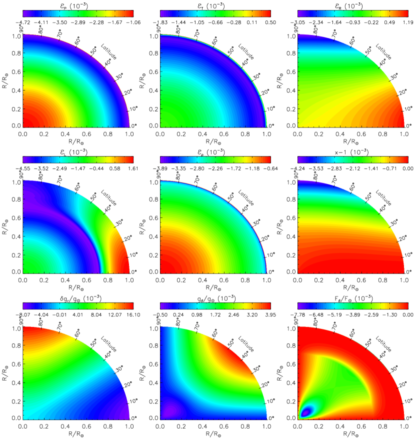
Figure 4: Contours of the 2D solar model with a uniform rotation rate $\Omega=10^{-4}$ s^-1. The top five sub-figures show the detail dependence of ${\cal E}_{P}$ to ${\cal E}_{\rho}$ on $R/R_{\sun}$ and $\theta$. The last fore sub-figures show the equipotential surface function $x-1$, the transverse component of energy flux ${\bf F}$, $F_{\theta}/F_{\sun}$, the radial perturbation component, and transverse component of the gravitational acceleration.

To see where the maximal rotation effect takes place, we plot ${\cal E}_{R}={\cal E}(m(R),\{\theta\};\Omega)$ as a function of $R/R_{\sun}$ and $\Omega$ in Fig. 3, where ${\cal E}_{R}$ is the maximal value among ${\cal E}_{P}$, ${\cal E}_{T}$, ${\cal E}_{r}$, ${\cal E}_{L}$ and ${\cal E}_{\rho}$ over all zones, and $R$ is the radius of the mass shell $m$ in the standard solar model. Similarly, we have ${\cal E}_{\theta}={\cal E}(\{m\},\theta;\Omega)$. Since it changes little with $\theta$, we do not need to plot it. Fig. 3 shows that the maximum takes place at the base of the convection zone or near the surface. Fig. 4 shows the detail dependence of ${\cal E}_{P}$, ${\cal E}_{T}$, ${\cal E}_{r}$, ${\cal E}_{L}$ and ${\cal E}_{\rho}$ on $R/R_{\sun}$ and $\theta$. It also shows the equipotential surface $x$, $F_{\theta}$, $\delta g_{r}$ and $g_{\theta}$, which have no 1D counterparts.

5.2.2 Uniform rotation-like magnetic field

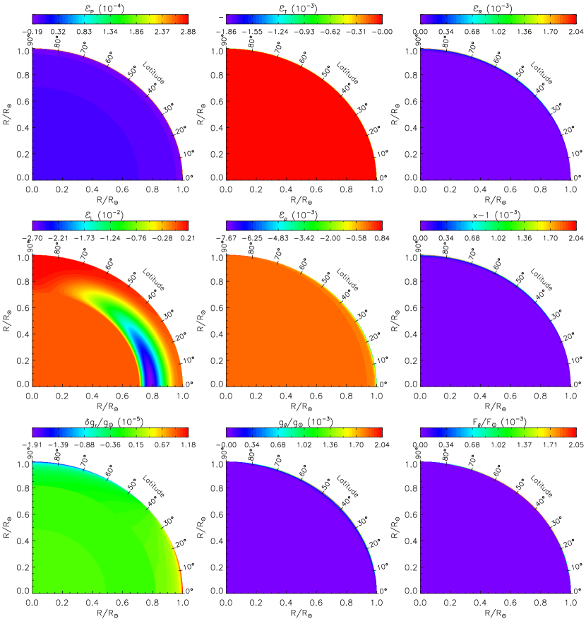
Figure 7: Contours of the 2D solar model with a uniform rotation-like toroidal magnetic field ${\bf B}=(0,0,(4\pi\rho)^{1/2}\Omega r\sin\theta)$, where $\Omega=10^{-6}$ s^-1. The top five sub-figures show the detail dependence of ${\cal E}_{P}$ to ${\cal E}_{\rho}$ on $R/R_{\sun}$ and $\theta$. The last fore sub-figures show the equipotential surface function $x-1$, the transverse component of energy flux ${\bf F}$, $F_{\theta}/F_{\sun}$, the radial perturbation component, and transverse component of the gravitational acceleration.

The uniform rotation-like toroidal magnetic field is ${\bf B}=(0,0,(4\pi\rho)^{1/2}\Omega r\sin\theta)$. We repeat the similar model calculations to rotation. Figs. 5 -7 show the results. Once again, the high-precision is achieved. Comparing them with Figs.2-4 we can see rotation-like magnetic fields affect stellar structures in a different way from the rotation: magnetic effects take place in the convection zone and peak near the surface. Rotation-like turbulence behaves like a rotation-like magnetic field.

5.2.3 Differential rotation-like magnetic field: torus

The torus field is a rotation-like toroidal magnetic field, ${\bf B}=(0,0,(4\pi\rho)^{1/2}\Omega r\sin\theta)$. The magnetic rotation rate $\Omega$ is defined in Appendix B. There are two torus tubes that are parallel to the equatorial plane since they are assumed to be symmetric with respect to the equatorial plane. As a result, there are four circles on any meridional plane.

Unlike the uniform rotation rate, we should first find out the discrete Fourier transform of the square of the differential rotation rate $\Omega$, $\Omega^{2}$, which is equally discretized in the range of $\theta$ from 0 to $\pi/2$, namely $\Omega_{i}$ for i = 0 to N. Here N should be a power of 2. We calculate $\Omega^{2}$ in the first quadrant and then extend it to the other three quadrants according to the symmetry described above. Its discrete Fourier transform $F_{n}$ are finally calculated by means of the Fast Fourier Transform (FFT) of a real function (See the subroutine realft.for given in Numerical Recipe) for n = 0 to 4N. Each pair of the data contain the real and imaginary parts of the FFT except for the first pair. The imaginary part vanishes since $\Omega^{2}$ is a real function of $\theta$, which is now in the range of 0 to $2\pi$. The odd components vanish due the equatorial symmetry. We use $y_{n}$ to denote the nonzero components. The nonzero $F_{n}$ contains $F_{0}$, which is twice the uniform component, $y_{0}=F_{0}/2$; and $F_{1}$, which stores the twice of the Nyquist critical wavenumber component, $y_{N}=F_{1}/2$; and the even components $y_{n}=F_{4n}$ for n = 1 to N-1. Consequently, we have

$$\Omega^{2}=\sum_{n=0}^{N}y_{n}\cos 2n\theta.$$ (114)

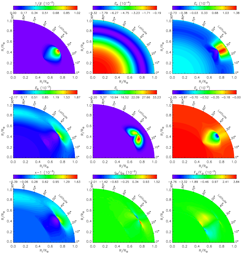
Figure 8: Contours of the 2D solar variability model with a torus field, in which the applied magnetic field (measured in the plasma $\beta$ parameter), the relative changes of the stellar structure variables (pressure, temperature, radius, luminosity and density) and the transverse components of the gravitational acceleration and flux vectors.

Fig. 8 contains nine sub-figures for the Gaussian profile defined in Appendix B, in which $\Omega_{0}=3\times 10^{-5}$. Sub-figure (1,1) shows the reciprocal of the plasma $\beta$ parameter as a function of ($R/R_{\sun},\theta$), which is defined as the ratio of the gas pressure over the magnetic pressure: $1/\beta=\frac{1}{2}\rho\Omega^{2}r^{2}\sin^{2}\theta/P$. Sub-figures (1,2)-(2,3) show ${\cal E}_{P}\sim{\cal E}_{\rho}$. The equipotential surface, the colatitudinal components of the gravitational acceleration vector and the flux vector are shown in the bottom panel, namely, sub-figures (3,1)-(3,3).

Sub-figure (1,2) shows that pressure does not vary with colatitude $\theta$ on the equipotential surface. It is the very feature that is required by the hydrostatic equilibrium on the surface. The numerical method of the solution to the 2D stellar structure equations presented in this paper is designed to achieve this feature. It is not trivial at all.

Sub-figure (1,3) indicates that the presence of the magnetic flux loop beneath the surface affects the temperature distribution in site and above. This is reasonable since the thermal time scale near the base of the convection zone (where the loop is located) is much longer than the solar cycle so that the temperature perturbation travels little inwards in the cyclic period. In contrast, it can substantially travel outwards in short time since the thermal timescale above the torus field is very small. Another feature for the 2D temperature effect is that the temperature increases above the buried field. We see sunspots in the solar active regions. It is well-known that sunspots reduce the energy output of the Sun. We also know that the active regions increase the net energy output of the Sun as a whole. The idea that the temperature increase caused by the buried fields over-compensates the sunspot is a natural explanation to the net increase of the energy output in the active regions of the Sun.

Sub-figures (2,1) and (3,1) are similar to each other. The distinction is their references: the former refers to the 1D radius of the equipotential surface, and the latter refers to the equatorial radius. The maximal radius change takes place at the minimal $\beta$ parameter. Both of them show the equipotential surface profile.

Comparing sub-figure (2,3) with (1,1) we can see that the density change inversely follows the plasma $\beta$ parameter and is of the same order of magnitude as $1/\beta$, which is in agreement with the analytical result: $(\rho\,-<\rho>)/<\rho>=1/(1+1/\beta)\approx-1/\beta$. The sub-figure also shows that the density decrease maximizes in the loop. This will give rise to a buoyant force on the loop in the radial direction. Its component on the plane that is parallel to the equator plane cancels out since the loop is azimuthally symmetric. Its component in the meridional direction will generate an acceleration in the same direction, $a_{m}$. Detailed calculation (see Appendix §B) shows $a_{m}\approx 32$ cm s^-2. The buoyant force is assumed to be balanced by the turbulent pressure generated by the down-flow plumes found in the realistic three-dimensional turbulent simulations of the solar convection zone near the surface of the Sun (e.g., Stein and Nordlund 1998; Robinson et al 2003). These simulations reveal that the up-flow and down-flow are not symmetric and the down-flow is stronger than the up-flow.

In the real Sun, this condition is obeyed until the magnetic field reaches a critical value whereby the buoyancy forces dominate, magnetic loops making up the torus float up, produce magnetic activity in the solar surface, and the toroidal field is depleted. We do not model these details in our code excepting in terms of the decrease of the toroidal field.

The transverse components of the gravitational acceleration vector ${\bf g}$ and the flux ${\bf F}$ shown in sub-figures (3,2) and (3,3) are purely 2D effects. Their characteristics and other 2D effects need to be investigated further and will be presented separately.

6 CONCLUSIONS

We present a new set of differential equations to describe the stellar equilibrium, in which two dimensional effects are explicitly taken into account. We improve the treatment presented in a previous paper of this series, by relaxing some approximations that had been made in that context; this task required one more differential equation, with the introduction of a new variable, i.e. the deviation of the radial component of gravity from the standard expression that is obtained when the Poisson equation is solved neglecting the angular derivatives.

We have shown that by selecting an appropriate convergence criterion our code can reach the precision required by current and forthcoming observations.

The code can now be used to test the effects of magnetic fields of any axisymmetric magnetic field configuration on the structure of the current Sun, and to investigate the change of the observable solar properties related to the variation of the magnetic field with the solar cycle. We have used the code to scan a very large region of the parameter space to test the code, and will present our findings in a separate paper.

Finally, we wish to emphasize that because we are interested in modeling the effects of a dynamo-type field on the detailed envelope structure and global properties of the Sun, the code has been optimized for short timescales phenomena (down to 1 yr). Consequently, the time dependence of the code has so far been tested exclusively to address such problems, and we can not assume that the code could be used to model long term stellar evolution without further modifications.

Appendix A COEFFICIENT MATRIX ELEMENTS

Eq. (98a) consists of a set of non-homogeneous linear algebraic equations. We work out these nonzero elements in this appendix.

A.1 Useful Partial Derivatives

The partial derivatives of the differential equations are required for the linearization. By defining the shorthand notation $\partial_{X}Y=\partial Y/\partial\log X$, we can calculate the useful derivatives as follows.

In fact, we need to calculate all the derivatives of ${\cal P}$, ${\cal T}$, ${\cal U}^{i}$ ($i=1,2,3,4,5$), ${\cal R}$, and ${\cal L}^{i}$ ($i=1,2$) with respect to $P^{\prime}$, $T^{\prime}$, $r^{\prime}$, $L$, and $U$, respectively. For the sake of completeness and conciseness, we write down all nonzero partial derivatives and formulas except for the same as in Paper I. The derivatives of ${\cal P}$, ${\cal T}$, and ${\cal L}^{1}$ are the same as in Paper I, where ${\cal L}^{1}$ is equivalent to ${\cal L}$ in Paper I.

The derivatives of ${\cal R}$ may be nonzero only for k = j and l = i - 1, i. The unique nonzero derivative is

$$\partial_{R}{\cal R}=-\cdot{\cal R},$$

which is different from Paper I.

The derivatives of ${\cal L}^{\ell}$ ($\ell=2,3$) may be nonzero not only for k = j and l = i - 1, i. For the sake of simplicity, we rewrite $F_{\theta}$ as follows:

$$F_{\theta}=(F^{1}+F^{2}+F^{3})\tilde{P},$$

where

$$F^{1} = -\frac{4acT^{4}\nabla}{3\kappa\rho}$$

$$F^{2} = -\frac{1}{2}\frac{\rho C_{P}Tl_{m}v_{\mbox{\scriptsize{conv}}}\nabla}{1+v_{\mbox{\scriptsize{conv}}}/v_{0}}$$

$$F^{3} = \frac{1}{2}\frac{\rho C_{P}Tl_{m}v_{\mbox{\scriptsize{conv}}}\nabla^{\prime}_{\mbox{\scriptsize{ad}}}}{1+v_{\mbox{\scriptsize{conv}}}/v_{0}}$$

$$\tilde{P} = \frac{GmQ\Lambda}{4\pi r_{e}^{4}P_{T}}.$$

In order to obtain the nonzero derivatives of $F_{\theta}$, we also need the following formulas:

$$\partial_{P}F^{1} = -F^{1}(\kappa_{P}+\alpha-\nabla_{P})$$

$$\partial_{T}F^{1} = -F^{1}(\kappa_{T}-\delta-\nabla_{T}-4)$$

$$\partial_{R}F^{1} = F^{1}\nabla_{R}$$

$$\partial_{L}F^{1} = F^{1}\nabla_{L}$$

$$\partial_{P}F^{2} = F^{2}(\alpha+\nabla_{P}+C_{\mbox{\scriptsize{PP}}})-\frac{v_{\mbox{\scriptsize{conv}}}/v_{0}}{1+v_{\mbox{\scriptsize{conv}}}/v_{0}}F^{2}(2\alpha+C_{\mbox{\scriptsize{PP}}}+\kappa_{P})$$

$$\partial_{T}F^{2} = F^{2}(1-\delta+\nabla_{T}+C_{\mbox{\scriptsize{PT}}})-\frac{v_{\mbox{\scriptsize{conv}}}/v_{0}}{1+v_{\mbox{\scriptsize{conv}}}/v_{0}}F^{2}(-2\delta+C_{\mbox{\scriptsize{PT}}}+\kappa_{T}-3)$$

$$\partial_{R}F^{2} = F^{2}\nabla_{R}$$

$$\partial_{L}F^{2} = F^{2}\nabla_{L}$$

$$\partial_{P}F^{3} = F^{3}(\alpha+\nabla^{\prime}_{P}+C_{\mbox{\scriptsize{PP}}})-\frac{v_{\mbox{\scriptsize{conv}}}/v_{0}}{1+v_{\mbox{\scriptsize{conv}}}/v_{0}}F^{3}(2\alpha+C_{\mbox{\scriptsize{PP}}}+\kappa_{P})$$

$$\partial_{T}F^{3} = F^{3}(1-\delta+\nabla^{\prime}_{T}+C_{\mbox{\scriptsize{PT}}})-\frac{v_{\mbox{\scriptsize{conv}}}/v_{0}}{1+v_{\mbox{\scriptsize{conv}}}/v_{0}}F^{3}(-2\delta+C_{\mbox{\scriptsize{PT}}}+\kappa_{T}-3)$$

$$\partial_{R}F^{3} = 0$$

$$\partial_{P}\tilde{P} = -\tilde{P}$$

$$\partial_{T}\tilde{P} = 0$$

$$\partial_{R}\tilde{P} = -4\tilde{P}$$

Here $\kappa_{P}\equiv\left(\frac{\partial\ln\kappa}{\partial\ln P_{T}}\right)_{T}$, $\kappa_{T}\equiv\left(\frac{\partial\ln\kappa}{\partial\ln T}\right)_{P_{T}}$, $C_{\mbox{\scriptsize{PP}}}\equiv\left(\frac{\partial\ln C_{P}}{\partial\ln P_{T}}\right)_{T}$, $C_{\mbox{\scriptsize{PT}}}\equiv\left(\frac{\partial\ln C_{P}}{\partial\ln T}\right)_{P_{T}}$, and $v_{0}=6acT^{3}/\rho^{2}C_{P}l_{m}\kappa$, $\nabla^{\prime}_{P}=(\partial\ln\nabla^{\prime}_{\mbox{\scriptsize{ad}}}/\partial\ln P_{T})_{T}$, and $\nabla^{\prime}_{T}=(\partial\ln\nabla^{\prime}_{\mbox{\scriptsize{ad}}}/\partial\ln T)_{P_{T}}$. As a result, we have

$$\partial_{P}F_{\theta} = \tilde{P}\sum_{\ell=1}^{3}\partial_{P}F^{\ell}+\partial_{P}\tilde{P}\sum_{\ell=1}^{3}F^{\ell}$$

$$\partial_{T}F_{\theta} = \tilde{P}\sum_{\ell=1}^{3}\partial_{T}F^{\ell}+\partial_{T}\tilde{P}\sum_{\ell=1}^{3}F^{\ell}$$

$$\partial_{R}F_{\theta} = \tilde{P}\sum_{\ell=1}^{2}\partial_{R}F^{\ell}+\partial_{R}\tilde{P}\sum_{\ell=1}^{3}F^{\ell}$$

$$\partial_{L}F_{\theta} = \tilde{P}\sum_{\ell=1}^{2}\partial_{L}F^{\ell}$$

$${\cal F} = \partial_{P}F_{\theta}+\partial_{T}F_{\theta}\cdot\nabla+\partial_{R}F_{\theta}\cdot\frac{\partial r^{\prime}}{\partial P^{\prime}}+\partial_{L}F_{\theta}\cdot{\cal L}/{\cal P}$$

where

$$\frac{\partial r^{\prime}}{\partial P^{\prime}}=-\frac{4\pi r_{e}^{3}P_{T}}{GmQx}.$$

These finish the expressions for ${\cal L}^{2}$ and ${\cal L}^{3}$, and their derivatives:

$$\partial_{P}{\cal L}^{2} = {\cal L}^{2}(F^{-1}_{\theta}\partial_{P}F_{\theta}-\alpha)$$

$$\partial_{T}{\cal L}^{2} = {\cal L}^{2}(F^{-1}_{\theta}\partial_{T}F_{\theta}+\delta)$$

$$\partial_{R}{\cal L}^{2} = {\cal L}^{2}(F^{-1}_{\theta}\partial_{R}F_{\theta}-1)$$

$$\partial_{L}{\cal L}^{2} = {\cal L}^{2}F^{-1}_{\theta}\partial_{L}F_{\theta}$$

$$\partial_{P}{\cal L}^{3} = -\alpha\cdot{\cal L}^{3}$$

$$\partial_{T}{\cal L}^{3} = \delta\cdot{\cal L}^{3}$$

$$\partial_{R}{\cal L}^{3} = -{\cal L}^{3}$$

After all nonzero components and their derivatives are calculated, we can sum them to obtain

$${\cal L} = \sum_{\ell=1}^{3}{\cal L}^{\ell}$$

$$\partial_{P}{\cal L} = \sum_{\ell=1}^{3}\partial_{P}{\cal L}^{\ell}$$

$$\partial_{T}{\cal L} = \sum_{\ell=1}^{3}\partial_{T}{\cal L}^{\ell}$$

$$\partial_{R}{\cal L} = \sum_{\ell=1}^{3}\partial_{R}{\cal L}^{\ell}$$

$$\partial_{L}{\cal L} = \partial_{L}{\cal L}^{2}$$

A.2 INTERIOR POINTS

The interior points can be grouped into four blocks:

Block I, l = i - 1 and k = j,

Block II, l = i and k = j.

A.2.1 w = P

For block I,

$$\frac{\partial F^{i}_{P}}{\partial R^{\prime}_{i-1}} = -\frac{1}{2}\Delta s_{i}\partial_{R}{\cal P}_{i-1}$$

$$\frac{\partial F^{i}_{P}}{\partial L_{i-1j}} = 0$$

$$\frac{\partial F^{i}_{P}}{\partial P^{\prime}_{i-1}} = -\frac{1}{2}\Delta s_{i}\partial_{P}{\cal P}_{i-1}-1$$

$$\frac{\partial F^{i}_{P}}{\partial T^{\prime}_{i-1j}} = 0$$

For block II,

$$\frac{\partial F^{i}_{P}}{\partial R^{\prime}_{i}} = -\frac{1}{2}\Delta s_{i}\partial_{R}{\cal P}_{i}$$

$$\frac{\partial F^{i}_{P}}{\partial L_{ij}} = 0$$

$$\frac{\partial F^{i}_{P}}{\partial P^{\prime}_{i}} = -\frac{1}{2}\Delta s_{i}\partial_{P}{\cal P}_{i}+1$$

$$\frac{\partial F^{i}_{P}}{\partial T^{\prime}_{ij}} = 0$$

A.2.2 w = T

For block I,

$$\frac{\partial F^{ij}_{T}}{\partial R^{\prime}_{i-1}} = -\frac{1}{2}\Delta s_{i}\partial_{R}{\cal T}_{i-1j}$$

$$\frac{\partial F^{ij}_{T}}{\partial L_{i-1j}} = -\frac{1}{2}\Delta s_{i}\partial_{L}{\cal T}_{i-1j}$$

$$\frac{\partial F^{ij}_{T}}{\partial P^{\prime}_{i-1}} = -\frac{1}{2}\Delta s_{i}\partial_{P}{\cal T}_{i-1j}$$

$$\frac{\partial F^{ij}_{T}}{\partial T^{\prime}_{i-1j}} = -\frac{1}{2}\Delta s_{i}\partial_{T}{\cal T}_{i-1j}-1$$

For block II,

$$\frac{\partial F^{ij}_{T}}{\partial R^{\prime}_{i}} = -\frac{1}{2}\Delta s_{i}\partial_{R}{\cal T}_{ij}$$

$$\frac{\partial F^{ij}_{T}}{\partial L_{ij}} = -\frac{1}{2}\Delta s_{i}\partial_{L}{\cal T}_{ij}$$

$$\frac{\partial F^{ij}_{T}}{\partial P^{\prime}_{i}} = -\frac{1}{2}\Delta s_{i}\partial_{P}{\cal T}_{ij}$$

$$\frac{\partial F^{ij}_{T}}{\partial T^{\prime}_{ij}} = -\frac{1}{2}\Delta s_{i}\partial_{P}{\cal T}_{ij}+1$$

A.2.3 w=R

For block I,

$$\frac{\partial F^{i}_{R}}{\partial R^{\prime}_{i-1}} = -\frac{1}{2}\Delta s_{i}\partial_{R}{\cal R}_{i-1}-1$$

$$\frac{\partial F^{i}_{R}}{\partial L_{i-1j}} = 0$$

$$\frac{\partial F^{i}_{R}}{\partial U_{i-1j}} = 0$$

$$\frac{\partial F^{i}_{R}}{\partial P^{\prime}_{i-1}} = -\frac{1}{2}\Delta s_{i}\partial_{P}{\cal R}_{i-1}$$

$$\frac{\partial F^{i}_{R}}{\partial T^{\prime}_{i-1j}} = -\frac{1}{2}\Delta s_{i}\partial_{T}{\cal R}_{i-1}$$

For block II,

$$\frac{\partial F^{i}_{R}}{\partial R^{\prime}_{i}} = -\frac{1}{2}\Delta s_{i}\partial_{R}{\cal R}_{i}+1$$

$$\frac{\partial F^{i}_{R}}{\partial L_{ij}} = 0$$

$$\frac{\partial F^{i}_{R}}{\partial U_{ij}} = 0$$

$$\frac{\partial F^{i}_{R}}{\partial P^{\prime}_{i}} = -\frac{1}{2}\Delta s_{i}\partial_{P}{\cal R}_{i}$$

$$\frac{\partial F^{i}_{R}}{\partial T^{\prime}_{ij}} = -\frac{1}{2}\Delta s_{i}\partial_{T}{\cal R}_{i}$$

A.2.4 w = L

For block I,

$$\frac{\partial F^{ij}_{L}}{\partial R^{\prime}_{i-1}} = -\frac{1}{2}\Delta s_{i}\partial_{R}{\cal L}_{i-1j}$$

$$\frac{\partial F^{ij}_{L}}{\partial L_{i-1j}} = 0$$

$$\frac{\partial F^{ij}_{L}}{\partial U_{i-1j}} = 0$$

$$\frac{\partial F^{ij}_{L}}{\partial P^{\prime}_{i-1}} = \frac{1}{2}\Delta s_{i}\partial_{P}{\cal L}_{i-1j}$$

$$\frac{\partial F^{ij}_{L}}{\partial T^{\prime}_{i-1j}} = -\frac{1}{2}\Delta s_{i}\partial_{T}{\cal L}_{i-1j}-1$$

For block II,

$$\frac{\partial F^{ij}_{L}}{\partial R^{\prime}_{i}} = -\frac{1}{2}\Delta s_{i}\partial_{R}{\cal L}_{ij}$$

$$\frac{\partial F^{ij}_{L}}{\partial L_{ij}} = 0$$

$$\frac{\partial F^{ij}_{L}}{\partial U_{ij}} = 0$$

$$\frac{\partial F^{ij}_{L}}{\partial P^{\prime}_{i}} = -\frac{1}{2}\Delta s_{i}\partial_{P}{\cal L}_{ij}$$

$$\frac{\partial F^{ij}_{L}}{\partial T^{\prime}_{ij}} = -\frac{1}{2}\Delta s_{i}\partial_{P}{\cal L}_{ij}+1$$

A.3 BOUNDARY POINTS

A.3.1 Center: w = R

Central boundary points have only block II for w = R:

$$\frac{\partial F^{1}_{R}}{\partial R^{\prime}_{1}} = 1$$

$$\frac{\partial F^{1}_{R}}{\partial L_{1j}} = 0$$

$$\frac{\partial F^{1}_{R}}{\partial U_{1j}} = 0$$

$$\frac{\partial F^{1}_{R}}{\partial P^{\prime}_{1}} = \frac{1}{3}\alpha_{01}$$

$$\frac{\partial F^{1}_{R}}{\partial T^{\prime}_{1j}} = -\frac{1}{3}\delta_{01}$$

A.3.2 Center: w = L

Central boundary points have block II for w = L:

$$\frac{\partial F^{1j}_{L}}{\partial R^{\prime}_{1}} = 0$$

$$\frac{\partial F^{1j}_{L}}{\partial L_{1j}} = 1$$

$$\frac{\partial F^{1j}_{L}}{\partial U_{1j}} = 0$$

$$\frac{\partial F^{1j}_{L}}{\partial P^{\prime}_{1}} = -\partial_{P}{\cal L}_{1j}$$

$$\frac{\partial F^{1j}_{L}}{\partial T^{\prime}_{1j}} = -\partial_{T}{\cal L}_{1j}$$

A.3.3 Surface: w = R

Surface boundary points have block I for w = R:

$$\frac{\partial F^{M+1}_{R}}{\partial R^{\prime}_{M}} = 1$$

$$\frac{\partial F^{M+1}_{R}}{\partial L_{Mj}} = 0$$

$$\frac{\partial F^{M+1}_{R}}{\partial U_{Mj}} = 0$$

$$\frac{\partial F^{M+1}_{R}}{\partial P^{\prime}_{Mj}} = -a_{1}$$

$$\frac{\partial F^{M+1}_{R}}{\partial T^{\prime}_{Mj}} = -a_{2}$$

A.3.4 Surface: w = L

Surface boundary points have block I for w = L:

$$\frac{\partial F^{M+1j}_{L}}{\partial R^{\prime}_{Mj}} = 0$$

$$\frac{\partial F^{M+1j}_{L}}{\partial L_{Mj}} = 1$$

$$\frac{\partial F^{M+1j}_{L}}{\partial U_{Mj}} = 0$$

$$\frac{\partial F^{M+1j}_{L}}{\partial P^{\prime}_{Mj}} = -L_{Mj}a_{4}$$

$$\frac{\partial F^{M+1j}_{L}}{\partial T^{\prime}_{Mj}} = -L_{Mj}a_{5}$$

Appendix B Buoyant acceleration of a magnetic flux loop in the meridional direction

The magnetic flux loop used in this paper is assumed to be axisymmetric with respect to the polar axis. Its buoyant force (${\bf f}_{B}$) is radial and can be decomposed into two components. One is parallel to the equatorial plane ($f_{e}$), and the other is perpendicular to it ($f_{m}$). The former is canceled out since the loop is axisymmetric with respect to the polar axis (i.e., $f_{e}=0$), and the latter is in the meridional direction ($f_{m}\neq 0$). In order to compute the buoyant acceleration of the loop in the meridional direction ($a_{m}=f_{m}/m_{L}$), we have to compute $f_{m}$ and the mass of the loop $m_{L}$.

We must first calculate the boundary of the loop. The polar axis is assumed to be the z-axis. The equation for a torus azimuthally symmetric about the z-axis in Cartesian coordinates is

$$(c-\sqrt{x^{2}+y^{2}})^{2}+(z-z_{0})^{2}=a^{2},$$ (B1)

where $c$ is the radius from the center of the hole to the center of the torus tube, $a$ is the radius of the tube, and $(0,0,z_{0})$ is the center point coordinate of the hole. In the xz-plane the torus becomes two circles. One of them is

$$(c-x)^{2}+(z-z_{0})^{2}=a^{2}$$ (B2)

in Cartesian coordinates. We need to determine its boundary. In the spherical polar coordinates ($r,\theta,\phi$), Eq. (B2) becomes

$$(c-r\sin\theta)^{2}+(r\cos\theta-c\cot\theta_{0})^{2}=a^{2},$$ (B3)

where $\theta_{0}$ is the colatitude of the center of the circle. The radius range of the circle for each $\theta$ is given by the solutions for $r$ of Eq. (B3): $r_{-}\leq r\leq r++$, where $r_{\pm}$ are defined by

$$r_{\pm}=c(\sin\theta+\cos\theta\cot\theta_{0})\pm c[(\sin\theta+\cos\theta\cot\theta_{0})^{2}-1-\cot^{2}\theta_{0}+a^{2}/c^{2}]^{1/2}.$$ (B4)

The colatitude range of the circle for each radius $r$ is determined by the solutions of Eq. (B3) for $\theta$:

$$\theta_{\pm}=\arccos\left[\frac{b\sin 2\theta_{0}\pm[b^{2}/\sin^{2}2\theta_{0}-4(b^{2}-1)\sin^{2}\theta_{0}]^{1/2}}{2}\right],$$ (B5)

where

$$b=\frac{c^{2}/\sin^{2}\theta_{0}+r^{2}-a^{2}}{2cr}.$$ (B6)

Since $\theta_{-}\geq\theta_{+}$, the boundary of Eq. (B2) can be expressed by

$${\cal C}:\hskip 11.38109ptr_{-}\leq r\leq r_{+},\mbox{ and }\theta_{+}\leq\theta\leq\theta_{-},\mbox{ and }0\leq\phi\leq 2\pi.$$ (B7)

We have two ways to define a torus field. One is to use the step function: $\Omega=\Omega_{0}$ within the loop confined by ${\cal C}$, but $\Omega=0$ outside the loop, where $\Omega_{0}$ is a constant. The other way is to use the Gaussian profile to smooth the step function: $\Omega=\Omega_{0}\exp[-\frac{1}{2}\frac{(\theta-\theta_{0})^{2}}{\sigma^{2}}]$, where $\sigma=\frac{1}{3}(\theta_{+}-\theta_{-})$.

We can then express the meridional buoyant force component $f_{m}$ and mass in the loop in terms of the following integrals:

$$f_{m} = 2\pi c\cos\theta_{0}\int_{\mbox{\scriptsize{{\cal C}}}}rg(<\rho>-\rho)drd\theta,$$ (B8)

$$m_{L} = 2\pi c\int_{\mbox{\scriptsize{{\cal C}}}}r\rho drd\theta.$$ (B9)

The acceleration equals $a_{B}=f_{m}/m_{L}$. Here $<\rho>$ is the averaged density over the colatitude $\theta$ from 0 to $\pi/2$.

Figure 1: The numerical accuracy of the 2D solar models with a zero-rotation rate as a function of convergence criteria. The symbols mark the data points.

Figure 2: Maximal rotation effect as a function of the rotation rate $\Omega$. The symbols mark the data points, and the dashed line shows the relative error estimate.

Figure 3: Maximal rotation effect in all zones as a function of both the rotation rate $\Omega$ and radius $R/R_{\sun}$.

Figure 5: Maximal rotation effect as a function of the rotation rate $\Omega$. The symbols mark the data points, and the dashed line shows the relative error estimate.

Figure 6: Maximal rotation effect in all zones as a function of both the rotation rate $\Omega$ and radius $R/R_{\sun}$.

References

• Antia et al. (1998) Antia, H. M., Basu, S., & Chitre, S. M. 1998, Mon. Not. Roy. Astron. Soc. 298, 543
• Bahcall et al (2006) Bahcall, J. N., Serenelli, A. M. & Basu, S., 2006, ApJS, 165, 400
• Gough et al (1996) D. O. Gough, A. G. Kosovichev, J. Toomre, E. Anderson, H. M. Antia, S. Basu, B. Chaboyer, S. M. Chitre, J. Christensen-Dalsgaard, W. A. Dziembowski, A. Eff-Darwich, J. R. Elliott, P. M. Giles, P. R. Goode, J. A. Guzik, J. W. Harvey, F. Hill, J. W. Leibacher, M. J. P. F. G. Monteiro, O. Richard, T. Sekii, H. Shibahashi, M. Takata, M. J. Thompson, S. Vauclair, and S. V. Vorontsov 1996, Sci, 272, 1296
• Li et al (2003) Li, L. H., Basu, S., Sofia, S., Demarque, P. & Guenther, D. B. 2003, ApJ, 591, 1267
• Li et al (2002) Li, L. H., Robinson, F. J., Demarque, P., Sofia, S. & Guenther, D. B. 2002, ApJ, 567, 1192
• Li et al (2006) Li, L. H., Ventura, P., Basu, S., Sofia, S. & Demarque, P. 2006, ApJS, 164, 215 (Paper I)
• Li & Sofia (2001) Li, L. H. & Sofia, S. 2001, ApJ, 549, 1204
• Lydon & Sofia (1995) Lydon, T.J. & Sofia, S. 1995, ApJS, 101, 357
• Prather (1976) Prather, M. J., 1976, Ph.D. thesis, Yale University (Appendix A)
• Robinson et al (2003) Robinson, F. J., Demarque, P., Li, L. H., Sofia, S., Kim, Y.-C., Chan, K.L., & Guenther, D. B. 2003, MNRAS, 340, 923
• Stein & Nordlund (1998) Stein, R. F., & Nordlund, Å 1998, ApJ, 499, 914
• Winnick et al (2002) Winnick, R. A., Demarque, P., Basu, S., & Guenther 2002, ApJ, 576, 1075
Refer to caption