Near-IR search for lensed supernovae behind galaxy clusters

Abstract

Aims. Powerful gravitational telescopes in the form of massive galaxy clusters can be used to enhance the light collecting power over a limited field of view by about an order of magnitude in flux. This effect is exploited here to increase the depth of a survey for lensed supernovae at near-IR wavelengths.

Methods. We present a pilot supernova search programme conducted with the ISAAC camera at VLT. Lensed galaxies behind the massive clusters A1689, A1835, and AC114 were observed for a total of 20 hours divided into 2, 3, and 4 epochs respectively, separated by approximately one month to a limiting magnitude $J\raise 1.29167pt\hbox{$<$}\kern-7.5pt{\lower 2.79857pt\hbox{$\sim$}}24$ (Vega). Image subtractions including another 20 hours worth of archival ISAAC/VLT data were used to search for transients with lightcurve properties consistent with redshifted supernovae, both in the new and reference data.

Results. The feasibility of finding lensed supernovae in our survey was investigated using synthetic lightcurves of supernovae and several models of the volumetric Type Ia and core-collapse supernova rates as a function of redshift. We also estimate the number of supernova discoveries expected from the inferred star-formation rate in the observed galaxies. The methods consistently predict a Poisson mean value for the expected number of supernovae in the survey of between N_SN=0.8 and 1.6 for all supernova types, evenly distributed between core collapse and Type Ia supernovae. One transient object was found behind A1689, $0.5\arcsec$ from a galaxy with photometric redshift $z_{\rm gal}=0.6\pm 0.15$. The lightcurve and colors of the transient are consistent with being a reddened Type IIP supernova at $z_{\rm SN}=0.59$. The lensing model predicts $1.4$ magnitudes of magnification at the location of the transient, without which this object would not have been detected in the near-IR ground-based search described in this paper (unlensed magnitude $J\sim 25$).

We perform a feasibility study of the potential for lensed supernovae discoveries with larger and deeper surveys and conclude that the use of gravitational telescopes is a very exciting path for new discoveries. For example, a monthly rolling supernova search of a single very massive cluster with the HAWK-I camera at VLT would yield $\raise 1.29167pt\hbox{$>$}\kern-7.5pt{\lower 2.79857pt\hbox{$\sim$}}10$ lensed supernova lightcurves per year, where Type Ia supernovae would constitute about half of the expected sample.

1 Introduction

Acting as powerful gravitational telescopes, massive galaxy clusters offer unique opportunities to observe extremely distant galaxies (Kneib et al., 2004), as well as distant supernovae (SNe), too faint to be otherwise detected (Kolatt & Bartelmann, 1998; Kovner & Paczynski, 1988; Sullivan et al., 2000; Gal-Yam et al., 2002; Gunnarsson & Goobar, 2003). Lensing magnifications of up to a factor $\sim$40 have been inferred for many multiple images of galaxies (Seitz et al., 1998) and typical magnification factors of 5 to 10 are common within the central few arcminutes of the most massive clusters of galaxies. Exploiting this remarkable boost in flux is an interesting avenue for probing the rate of exploding stars at redshifts beyond the detection capabilities of currently available telescopes. Successful programs detecting intermediate to high redshift SN at optical wavelengths include SDSS-II (Frieman et al., 2008), SNLS (Astier et al., 2006), and ESSENCE (Miknaitis et al., 2007), which all target $z\raise 1.29167pt\hbox{$<$}\kern-7.5pt{\lower 2.79857pt\hbox{$\sim$}}1$ supernovae, mainly Type Ia. For higher redshifts, Riess et al. (2007) demonstrated the power of space measurements by reporting the discovery and analysis of 23 Type Ia SNe with $z\geq 1$, although not without significant effort. The project made use of about 750 HST orbits to detect SNe, obtain multi-color lightcurves and grism spectroscopy with ACS and NICMOS. Dawson et al.(in prep.) improved the yield of high-$z$ Type Ia SN detections with ACS/HST by targeting SN in massive $z>1$ clusters. A common feature of both HST projects was that the search was done in the F850LP filter, i.e., $z$-band. Poznanski et al. (2007) used the extremely large FoV of the Suprime-Cam at Subaru 8.2m to measure SNIa rates up $z=1.6$. They reported the discovery of 13 SNIa beyond $z=1$ with repeated imaging of the Subaru Deep Field at optical wavelengths, including $z$-band.

We explore a complementary technique for SN detection and photometric follow-up that involves a near-IR, “rolling”, SN survey behind intermediate-redshift massive clusters. By exploiting the significant lensing magnification, the redshift discovery limit is enhanced. There are, however, two main limitations to this approach. First, the large lensing magnification is limited to small solid angles around the cluster core, of typically a few arc-minutes. Second, conservation of flux implies that the survey area behind the cluster in the source plane is shrunk due to lensing.

The choice of near-IR filter ensures that the survey has a potential for SNIa discoveries to unprecedented high redshifts, $z\sim 2.5$, and still samples the rest-frame optical part of the spectrum, potentially allowing a significant increase in the lever arm of the Type Ia SN Hubble diagram. Furthermore, because of the strong lensing effect, multiple images of high$-z$ SNe with time separations of between weeks and a few years could be observed. These rare events could provide strong constraints on the Hubble constant, using the time-delay technique (Refsdal, 1964) and possibly be used as tests of dark matter and dark energy in an unexplored redshift range (Goobar et al., 2002; Mörtsell & Sunesson, 2006). A feasibility study of the potential for improving the mass models of clusters of galaxies using lensed SNe will be presented in Riehm et al., in preparation (Paper III).

In this paper, we describe a pilot program using the ISAAC near-IR imaging camera at ESO’s Very Large Telescope (VLT), to detect gravitationally lensed SNe behind very massive clusters of galaxies. The potential for a scaled-up version of this project with the new HAWK-I near-IR instrument at VLT is also studied. A description of the observing strategy, the data-set and data reduction, as well as a full presentation of the photometry of the transient object discussed in Sect. 6.2, are presented in an accompanying paper (Stanishev et al. (2009), Paper I).

Throughout this paper, we adopt the concordance model cosmology, $\Omega_{\rm M}=0.3$, $\Omega_{\Lambda}=0.7$, $h=0.7$, $w=-1$. Magnitudes are given in the Vega system.

2 Supernova subtypes

SN explosions are broadly divided into two classes, core-collapse supernovae (SN CC), marking the end of very massive stars ($\raise 1.29167pt\hbox{$>$}\kern-7.5pt{\lower 2.79857pt\hbox{$\sim$}}8M_{\sun}$), and the so-called Type Ia supernovae (SNIa), believed to be either the result of merging white dwarfs or accreting white dwarfs in close binaries, where thermonuclear explosions are triggered when the system is close to the Chandrasekhar mass, $1.38M_{\sun}$.

Several subtypes of explosions belong to the core-collapse class, including Type II SN as well as Type Ib/c and hypernovae (HN), which are also interesting because of their association with GRBs. Type II SNe are furthermore subdivided into IIP, IIL, and IIn based on lightcurve and spectroscopic properties. For reviews of SN classification and their general properties, see Filippenko (1997) and Leibundgut (2008).

In Table 1, we summarize some of the main properties of the SNe being considered in this analysis, which are: the peak $V$-band brightness, $M_{V}$; the one-standard-deviation range around the peak intrinsic luminosity, $\sigma_{M_{V}}$ (a Gaussian distribution has been assumed for all types, except for Type IIL supernovae, for which a bi-Gaussian distribution is used, with the two peak values being labeled IIL and IIL_bright ); and the fraction of the core-collapse SN subtypes, $f_{CC}$, inferred from measurements of the local universe. We adopted the values of $f_{CC}$, lightcurve and spectral properties compiled by Peter Nugent, which in turn are based on work by Richardson et al. (2002). We note, however, that the uncertainty in the relative fractions within the core-collapse types is quite large. For instance, Smartt et al. (2009) found a much higher fraction of Type Ib/c (29%) than Richardson et al. (2002), while their estimate of the number of type IIL is about a factor 10 lower than what has been assumed here. Clearly, significantly larger data-sets are needed to determine the CC rates accurately, both at low and high redshifts.

Since the peak brightness, lighcurve shape and spectral energy density vary significantly between SN types, we treat each subtype separately when computing the expected rates. Synthetic lightcurves of SNe at a luminosity distance $d_{L}(z)$ are calculated for the observer NIR filters using cross-filter K-corrections (Kim et al., 1996)

$$m_{Y}(z,t)=M_{V}(t)+{\cal D}(z)+K_{V{Y}}(z,t)+\Delta m(z),$$ (1)

where $Y$ represents an arbitrary observer filter and the distance modulus is defined as

$${\cal D}(z)=25+5\log_{10}{\left(d_{L}(z)\over 1{\rm Mpc}\right)}\,.$$ (2)

The luminosity distance, $d_{L}$, in a flat ($\Omega_{K}=0$) Friedmann-Lemaître-Robertson-Walker model of the universe is given by:

$$d_{L}(z)=c(1+z)\int_{0}^{z}{{\rm d}z^{\prime}\over H(z^{\prime})},$$ (3)

where $c$ denotes the speed of light in vacuum and the Hubble parameter evolves with redshift as

$$H(z)=100\cdot h\sqrt{\Omega_{M}(1+z)^{3}+\Omega_{\Lambda}}\ ,$$ (4)

in units of ${\rm{\ km\ s^{-1}Mpc^{-1}}}$.

We also included in Eq. 1 the perturbation $\Delta m(z)=\Delta m_{\rm ext}(z)+\Delta m_{\rm lens}(z)$ in the observed magnitude from lensing magnification, $\Delta m_{\rm lens}$, and/or extinction by dust along the line of sight, $\Delta m_{\rm ext}$.

Table 1: Supernova properties.

SN type	$M_{V}\ (\rm mag)$	$\sigma_{M_{V}}\ (\rm mag)$	$f_{CC}$
Ia	-19.23	0.30
IIP	-16.90	1.12	0.50
IIL	-17.46	0.38	0.2025
IILbright	-19.17	0.51	0.0675
IIn	-19.05	0.50	0.05
Ib/c	-17.51	0.74	0.15
HN	-19.20	0.30	0.03

Figure 1 shows examples of synthetic lightcurves for a representative set of SN types at redshifts $z=1.5$ and $z=2.0$ through the ISAAC $SZ$-filter ($\lambda_{eff}=1.06$ $\mu$m; FWHM$=0.13$ $\mu$m), a broader and redder version of the more common $Y$ filter. Due to the large lensing magnifications from the foreground cluster (Sect. 4.1), significantly higher redshifts can be probed, not only for the intrinsically fainter core-collapse supernovae, but also for Type Ia supernovae beyond $z\sim 1.5$.

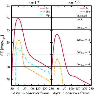
Figure 1: Synthetic lightcurves in $SZ$-band of Type Ia, Type Ib/c, and Type IIP supernovae at $z=1.5$ and $z=2$ at their mean peak brightness. Also shown is the increased sensitivity for lensing magnification by 1, 2, 3 and 4 mag. The unlensed limit, $\sim 24$, corresponds to the search depth for most of the data in Table 3. Type IIP supernovae are too faint to be detected with the ISAAC survey at $z=2$, even with $\Delta m_{\rm lens}=-4$.

3 Supernova rates

We now consider two different routes for computing the expected number of SNe in a survey. In Sect. 3.1, the volumetric approach is followed, i.e., the predictions are derived from the volume probed in the field of view of the survey and assumptions about the SN rate per co-moving volume for the various types of SNe as a function of redshift. In Sect. 3.2, we also consider the rates derived from the rest-frame UV luminosities of the resolved galaxies behind the clusters based on the assumption that they trace the star-formation rate in each individual galaxy.

3.1 Volumetric rate estimate

The expected number of SNe of a certain subclass, ${\rm d}N_{j}$, in a redshift interval, ${\rm d}z$, depends on the monitoring time for that specific SN type, $T_{j}$, the solid angle of the survey, $\omega$, and the volumetric SN rate, $r^{j}_{V}$ (with units Mpc^-3yr^-1), given by

$${\rm d}N_{j}=T_{j}(z)\cdot{r^{j}_{V}(z)\over(1+z)}\cdot dV_{C},$$ (5)

Furthermore, it is a function of cosmological parameters, since it includes the comoving volume element

$$dV_{C}={cd_{L}^{2}(z)\over H(z)(1+z)^{2}}\omega\ {\rm d}z.$$ (6)

Next, we explore the current estimates of the volumetric rates of core-collapse and Type Ia supernovae.

3.1.1 Core-collapse SNe

Large scale SN programs such as SDSS, SNLS, ESSENCE, or GOODS/PANS and even the planned survey at the LSST are rather inefficient at detecting core-collapse SNe at $z>1$. As an example, the two highest-redshift identified CC SNe in the five-year SNLS survey are at $z=0.617$ (a probable Ib/c) and $z=0.605$ (Ib/c confirmed). We note, however, that SNLS specifically targeted Type Ia supernovae, and thus not optimized for finding CC SNe.

The magnification provided by foreground clusters could enable the exploration of this population for the first time. Since the progenitors of CC SNe are massive short-lived stars, the CC SN rate, $r^{CC}_{V}$, reflects the ongoing star-formation rate (SFR, units $M_{\sun}$yr^-1Mpc^-3). Thus, we can use the SNR to obtain independent bounds on the cosmic SFR since

$$r^{CC}_{V}(z)=k_{8}^{50}\times{\rm SFR}(z),$$ (7)

where $k_{8}^{50}=0.007M^{-1}_{\sun}$ is estimated using a Salpeter IMF (Salpeter, 1955) and a progenitor mass range of between 8 and 50 solar masses, as in Dahlen et al. (2004). Although straightforward in principle, large uncertainties plague the procedure outlined in Eq. (7). The estimates of ${\rm SFR}(z)$ from various data sets show a large span (Chary & Elbaz, 2001; Giavalisco et al., 2004; Hopkins & Beacom, 2006; Mannucci et al., 2007), thus leading to a very uncertain range of predictions for the SN rates, as shown in Fig. 2, but also allowing for the possibility to constrain the ${\rm SFR}(z)$ by measuring $r^{CC}_{V}$. The estimate by Mannucci et al. (2007) (M07) shown in Fig.2 incorporates a strong efficiency cut due to dust obscuration. The underlying assumption is that star formation correlates with dust density. Thus, as the star formation increases with redshift, the fraction of obscured SNe increases. M07 parametrized the fraction of observable CC SNe at optical wavelengths as being $f=0.95-0.28\times z$ for $z\leq 2$. In a similar way to the approach followed by Lien & Fields (2009), the CC rate in M07 is extended smoothly up to $z\sim 4$ in a manner compatible with the upper limits on the fraction of radiation escaping high-redshift galaxies, $f\sim 0.02$ for the redshift interval $3<z<9$ (Gnedin et al., 2008). While this is a rather conservative approach, given that these estimates were derived for considerably shorter rest-frame wavelengths than those relevant to our work, it has a negligible impact on our results.

The observational results for the CC rates at high-$z$ (Dahlen et al., 2004) show an increase in the range $z\sim 0.3-0.7$, which is consistent with independent estimates of the SFR. Extending these measurements to $z\geq 1$ is clearly important for checking the underlying SFR models. Observations at near-IR, i.e. in the rest-frame optical, should also provide a direct probe of the star formation that could be missed by UV surveys due to extinction by dust along the line of sight. Since the VLT/ISAAC survey had very limited sensitivity beyond $z>2$, the smoothly extrapolated model of M07 is used mainly for our estimate of the feasibility of discovering lensed SNe in future surveys in Sect. 7.

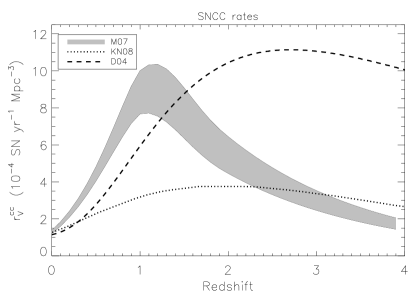
Figure 2: Predictions for the CC SN rate, $r^{CC}_{V}(z)$ derived from various estimates of the star formation rate, ${\rm SFR}(z)$. The shaded region (M07) is an extrapolation based on the dust corrected rate in Mannucci et al. (2007). The dashed line (D04) gives the best fit to the GOODS CC discoveries, as shown in Dahlen et al. (2004). The dotted line (KN08) shows the prediction in Kobayashi & Nomoto (2008).

3.1.2 Type Ia SNe

While SNIa have been used extensively for deriving cosmological parameters, it is unsatisfactory that the progenitor scenario preceding the SN explosion is still mostly unknown. Existing models predict that different scenarios, such as the single degenerate and the double degenerate models, should have different delay-time distributions $\phi(t)$, describing the time between the formation of the progenitor star and the explosion of the SN. The results of Mannucci et al. (2005) and Sullivan et al. (2006) suggest that the specific SNR (SNR per unit mass) is significantly higher in young star forming galaxies than in older galaxies. Pritchet et al. (2008) used the results from Sullivan et al. (2006) to show that the delay-time distribution, $\phi(t)$, is consistent with a power-law function and that the specific SNR is at least a factor of 10 higher in active star-forming galaxies compared to passive galaxies.

Using a different method, Strolger et al. (2004) compare the SFR(t) and the SNR, $r^{Ia}_{V}(t)$, derived in the GOODS fields to derive the delay-time distribution with the relation

$$r^{Ia}_{V}(t)=\nu\cdot\int_{0}^{t}{\rm SFR}(t^{\prime})\,\phi(t-t^{\prime})\,{\rm d}t^{\prime},$$ (8)

where $\nu$ is the number of SNe per unit stellar mass formed. Assuming that $\phi(t)$ has a Gaussian shape, they found a preferred delay time of $\tau\sim$3-4 Gyr, which is significantly longer than that found when using the specific SNR described above.

We note that the main driver of the relatively long delay-time found in the method used by Strolger et al. (2004) is the low number of Type Ia SNe found at high redshift $z>1.4$. Using the extended GOODS survey, Dahlen et al. (2008) also found fewer Type Ia SNe at $z>1.4$ than what is expected if the delay-time is short and SNR follows the SFR. Results for the Type Ia rate at $z>$1.4 were also presented in Poznanski et al. (2007) and Kuznetsova et al. (2008). While both these sets of results show a rate that is consistent with being constant at $z>1.4$, the large statistical errors can not exclude a rate that declines sharply as suggested by the results in Dahlen et al. (2008).

It is therefore particularly important to search for SNe at these redshifts, where the predicted rate is most sensitive to the delay time. If $\tau$ is large ($>$3-4 Gyr), there should be a steep decline in the SNIa rate at $z>$1.5, while if $\tau$ is short, the SNR should follow the SFR and remain fairly constant to $z\raise 1.29167pt\hbox{$>$}\kern-7.5pt{\lower 2.79857pt\hbox{$\sim$}}3$.

Furthermore, there are also theoretical predictions that the SNIa rate could be significantly suppressed (or even inhibited) at high redshifts ($z>2$ in spirals and $z>2.5$ in ellipticals) due to metallicity effects, e.g., Kobayashi et al. (1998). Kobayashi & Nomoto (2008) revised their analysis and found an expected increase of the SNIa rate in elliptical hosts above $z=2.5$. These results also show that deriving the Type Ia rate at high redshift is of great interest.

To calculate the number of detectable Type Ia SNe, we use a sample of SNIa rate model predictions and best-fit solutions to the available data, extrapolated to very high redshifts. These models are shown in Fig. 3. As for CC SNe, we used the smoothly extrapolated M07 model as a benchmark for the feasibility studies in Sect. 7.

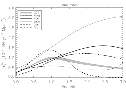
Figure 3: Extrapolations of available SNIa rate predictions, $r^{Ia}_{V}(z)$. The shaded region (M07) is an extrapolation based on the dust corrected rate in Mannucci et al. (2007). The dashed line (D08) gives the best fit to the HST supernova survey (Dahlen et al., 2008) corresponding to $\tau=3.4$ Gyr. The dot-dash line (TAU1) shows the corresponding rate for $\tau=1.0$ Gyr. In both cases, a Gaussian distribution was assumed for $\tau$. The thick solid line (N06) corresponds to the SNLS published rates in Neill et al. (2006). The thin solid line (SB05) stems from the so-called “A+B model” in Scannapieco & Bildsten (2005) and the dotted line (KN08) shows the prediction in Kobayashi & Nomoto (2008).

3.2 SN rates derived from the SFR of observed galaxies

Since the rate of SNe is expected to follow the star-formation rate, we also consider the numbers that can be derived for the SFR in the galaxies detected along the field of view. In Sect. 5, we describe how galaxy catalogs were generated for the resolved objects along the line of sight to massive clusters.

We used the rest-frame UV luminosity as a tracer of the SFR in the observed galaxies, redshifted to the optical bands. Since the UV luminosity is dominated by the most short-lived stars, it is closely related to star formation.

We use $L_{2800}$, the flux at rest-frame $\lambda_{eff}=2800\AA$, to estimate the SFR. We first used the photometric (or spectroscopic) redshift (see Sect. 5) to derive which two observed filters straddle the rest-frame $L_{2800}$ and interpolate between those using the best-fit spectral template to derive the apparent magnitude corresponding to the rest-frame $L_{2800}$ flux. The absolute $L_{2800}$ magnitude is thereafter derived after correcting for distance modulus and K-corrections. Next, the lensing magnification is taken into account, as described in Sect. 4.1.

Finally, we use the relation between $L_{2800}$ and SFR from (Dahlen et al., 2007) to relate the flux to star formation,

$${\rm SFR}(M_{\odot}{\rm yr}^{-1})={L_{2800}({\rm erg\cdot s}^{-1}{\rm Hz}^{-1})\over 7.0\cdot 10^{27}}.$$ (9)

The expected number of core collapse SNe are calculated using Eq. (7), whereas the SNIa rate is estimated using Eq. (8) for a Gaussian distribution of $\phi(t)$ with $(\tau,\sigma)=(3.4,0.68)$ in units of Gyr.

4 Clusters as gravitational telescopes

We have investigated the use of some of the most massive clusters of galaxies as gravitational telescopes; A1689, A1835, and AC114. A1689 ($z=0.183$) has the largest Einstein radius of all massive lensing clusters, $\theta_{E}\sim 50\arcsec$. Broadhurst et al. (2005) and Limousin et al. (2007) performed a strong lensing analysis using HST data and identified 115 images of 34 multiply lensed background galaxies in the redshift range $1<z<5.5$ based on spectroscopic and photometric redshift estimates. A cluster mass model of AC114 ($z=0.312$, $\theta_{E}\sim 30\arcsec$) and several strongly lensed sources, including a 5-image configuration at $z=3.347$ were presented in Campusano et al. (2001). The mass model for A1835 ($z=0.253$) yields an Einstein radius of $\theta_{E}\sim 40\arcsec$ at high-$z$ (Richard et al., 2006).

4.1 Lensing magnification: tunnel vision

To calculate the lensing magnification of the SN lightcurves, the public LENSTOOL software package was used. The code is specifically developed for modeling the mass distribution of galaxies and clusters in the strong and weak lensing regime (Kneib et al., 1996). It uses a Monte Carlo Markov Chain technique (Jullo et al., 2007) to constrain the parameters of the cluster model using observational data of the background galaxies as input. The output can then be used to compute, e.g., the magnification and time delay function at any given position behind the cluster. For A1689 the mass model by Limousin et al. (2007) was used. The clusters A1835 and AC114 were modeled as in Richard et al. (2006). Figure 4 shows the average lensing magnification as a function of source redshift in the FOV of the ISAAC camera, which is 2.5 $\times$ 2.5 arcmin² for the three cluster fields considered. We note that A1689 seems to be the most promising gravitational lens for reaching the highest redshifts. For the 2007 observations of A1689 centered on the cluster itself, the magnification is on average, $>$$\sim$2.5 mag for $z\raise 1.29167pt\hbox{$>$}\kern-7.5pt{\lower 2.79857pt\hbox{$\sim$}}1$ in the ISAAC field of view. The 2003/2004 archival observations that we used were offset from the cluster core, and therefore the average magnification for these observations is lower, $\sim$1.5 mag for $z\raise 1.29167pt\hbox{$>$}\kern-7.5pt{\lower 2.79857pt\hbox{$\sim$}}$1. For A1835, the average magnification is $\sim$1 mag for $z\raise 1.29167pt\hbox{$>$}\kern-7.5pt{\lower 2.79857pt\hbox{$\sim$}}1$. The width of the A1689 2003/2004 and A1835 curves indicate the slightly different pointings and effective FOV of these observations. AC114 has an average lensing magnification of $\sim$0.8 mag for $z\raise 1.29167pt\hbox{$>$}\kern-7.5pt{\lower 2.79857pt\hbox{$\sim$}}1$.

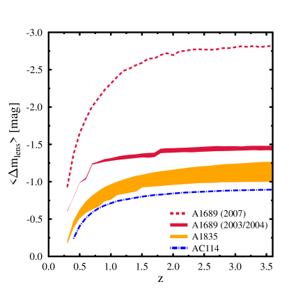
Figure 4: Average lensing magnification versus redshift for the three observed clusters computed with LENSTOOL (see text) for the ISAAC/VLT field of view. Two curves are shown for A1689, since the pointings in 2003/2004 (dashed red) and 2007 were different. The width of the curve for the A1689 pointings (solid red) in 2003/2004 and the A1835 pointings (orange) indicate that these pointings do not cover the same area, but are slightly shifted between observations and the effective area observed is different (details can be found in Paper I).

4.2 Monitoring time for SN surveys with gravitational telescopes

Because of flux conservation, large lensing magnifications result in small observed solid angle $\omega$.

Therefore, unlike other SN searches, the effective solid angle $\omega$ in Eq. (6) is not constant with redshift when cluster fields are targeted. The light beam at any given redshift behind the cluster is magnified by a factor

$$\mu=10^{-{0.4\cdot\Delta m_{\rm lens}}},$$ (10)

at the expense of a smaller solid angle $\widetilde{\omega}$ of viewing

$$\delta\widetilde{\omega}={\delta\omega_{0}\over\mu}={\delta\omega_{0}\cdot 10^{0.4\cdot\Delta m_{\rm lens}}},$$ (11)

where $\delta\widetilde{\omega}$ and $\delta\omega_{0}$ represent infinitesimal solid angle elements, with and without lensing magnification. Therefore, the effective volume of a lensed SN search ${\rm d}\widetilde{V}_{C}$ can be measured by substituting the expression into Eq. (6)

$${\rm d}\widetilde{V}_{C}={cd_{L}^{2}(z)\over H(z)(1+z)^{2}}\widetilde{\omega}\ {\rm d}z.$$ (12)

The corresponding reduction in the source area as a function of redshift for the strongest (A1689) and weakest (AC114) lens in our survey are shown in Fig. 5.

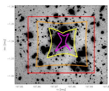
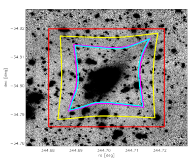
Figure 5: Source plane area shrinkage behind our strongest gravitational telescope A1689 (top figure) for various redshifts; $z=$0.25 (orange), 0.5 (yellow), 2.0 (magenta) and the weakest in the current survey AC114 (bottom figure) for various redshifts ($z=$ 0.5 (yellow), 2.0 (magenta), 3.0 (cyan). The utmost line (red) shows the effective FOV of the observations.

Although A1689 is the the most promising gravitational lens, the figures illustrate that the rapid shrinkage in the solid angle with increasing redshift is also very strong.

Thus, as shown in Gunnarsson & Goobar (2003), a gravitational lens does not always enhance the number of SN discoveries. However, it does increase the limiting redshift of a magnitude-limited survey. We exploit this effect to search for SNe at redshifts beyond those explored by “traditional” SN searches.

Weaker lenses, such as AC114 and A1835, may not go as deep in redshift, but one may still find a comparable number of SNe as behind A1689 (or even more), although these SNe would be found at somewhat lower average redshifts.

For the unlensed case, the monitoring time above threshold for a SN of type $j$, $T_{j}$, is a function of the SN lightcurve, the detection efficiency, $\epsilon$, the extinction by dust, $\Delta m_{\rm ext}$, and the intrinsic brightness $M_{j}$ with the probability distribution $P(M_{j})$. With $\Delta t_{j}$ being the lightcurve time period when the supernova is above the detection threshold,

$$T_{j}(z,\Delta m_{\rm ext})=\epsilon\cdot\int{\Delta t_{j}(z,M_{j}+\Delta m_{\rm ext})\,{P(M_{j})}{\rm d}M_{j}}.$$ (13)

We assume $P(M)$ to be Gaussian, and to have the mean values and standard deviations listed in Table 1.

Taking into account the lensing effect of the clusters, the monitoring time becomes

$$T_{j}(z,\Delta m_{\rm ext},\Delta m_{\rm lens})=\hskip 99.58464pt$$

$$\epsilon\cdot\int{\Delta t_{j}(z,M_{j}+\Delta m_{\rm ext}+\Delta m_{\rm lens})\,{P(M_{j})}{\rm d}M_{j}},$$ (14)

keeping in mind that $\Delta m_{\rm ext}>0$ corresponds to dimmed SNe. Usually, $\Delta m_{\rm lens}<0$, and SNe will be magnified (although there are also areas of the field where the gravitational lens demagnifies).

Thus, the expected number of SNe for a given type $j$, using volumetric rates, is then given by

$$N_{j}=\int T_{j}(z,\Delta m_{\rm ext},\Delta m_{\rm lens})\cdot{r^{j}_{V}(z)\over(1+z)}\cdot{\rm d}\widetilde{V}_{C},$$ (15)

where we assume an overall Milky-Way-like dust extinction (Cardelli et al., 1989) with $E(B-V)=0.15$ and $R_{V}=3.1$. In this study, we have assumed a constant optical depth for all supernovae. This choice matches the assumptions used to derive the SFR estimates that we have used.

5 Properties of background galaxies

For each one of the three considered clusters, galaxy catalogs were compiled using archival optical and near-IR photometry. The different instruments and filters are listed in Table 2.

The observed magnitudes in at least three bands, optical or near-IR, were used to derive a photometric redshift using the template-fitting technique (e.g., Gwyn (1995); Mobasher et al. (1996)). The software used is the code developed by the GOODS team as described in Dahlen et al. (2005; 2009, in prep.)

Figure 6 shows the distribution of galaxies in bins of $\Delta z=0.5$ for the three clusters. Furthermore, the restframe UV-flux at $2800$Å of each resolved galaxy was computed and used as a tracer of the SFR. Similarly, the integrated SFR was calculated in each redshift bin by summing the resolved galaxies behind each cluster. Thus, we compute the expected number of SNe with two methods: 1) the volumetric rate taken from the literature, and 2) the measured star-formation rate of the resolved galaxies in the FOV.

Table 2: Archival data used to calculate photometric redshifts.

Filter	Instrument/Camera
Abell 1689
F475W, F625W, F775W, F850LP	HST/ACS
F110W, F160W	HST/NICMOS
Abell 1835
V, R, I,	CFHT/CFH12K
F702W	HST/WFPC2
Z	VLT/FORS2
SZ, J, H, Ks	VLT/ISAAC
AC114
U	CTIO
B	AAT/CCD1
V	ESO-NTT
F702W, F814W	HST/WFPC2
J, H, Ks	VLT/ISAAC

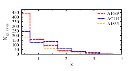
Figure 6: Resolved galaxies vs redshift behind A1689, A1835 and AC114.

6 The ISAAC pilot survey

During the spring of 2007, three clusters, A1689, AC114 and A1835, were monitored with the ISAAC instrument at VLT of approximately one-month intervals, as shown in Table 3. In total, the data set consists of 20 hours of VLT time on target: 4.5 hr, 5.85 hr and 10 hr for A1689, AC114 and A1835 respectively. The data is complemented by archival data (also listed in the table): 8.4 hr, 5.7 hr and 6.1 hr for A1689, AC114 and A1835. The survey filters in our 2007 program were chosen to match the deepest reference images. Thus, the SN search was done using the $SZ$-filter for A1689 and A1835 and $J$-band for AC114. A full description of the data reduction, SN search efficiency, and limiting magnitude is reported in Paper I. An average discovery depth at 90 % CL of $SZ,J\,\raise 1.29167pt\hbox{$<$}\kern-7.5pt{\lower 2.79857pt\hbox{$\sim$}}\,24$ mag (Vega) was derived by Monte Carlo simulations in which artificial stars were added to the images.

Table 3: Data used for transient search.

Date	Exposure	Seeing	90% detection	Areac
	[min]	[arcsec]	efficiency [mag]	[arcmin2]
Abell 1689 – VLT/ISAAC $SZ$-band
2003 02 09b	159	0.52	24.28, transient	3.70
2003 04 27	43	0.43	transient
2004 01 13	43	0.52	23.58, non-detect
2004 02 14	43	0.58	23.64, non-detect
2003 01 16	43	0.58	23.48	3.72
2003 02 15	43	0.50	23.60
2003 04 27	86	0.44
2004 01 12	43	0.55	23.64
2007 04 08	117	0.64	23.95	4.44
2007 05 14/15	117	0.65	23.95
2007 06 06	39	0.70	23.15
AC 114 – VLT/ISAAC $J$-band
2002 08 20	108	0.49	23.87	5.06
2007 07 13a	234	0.43	24.04
2007 08 09	117	0.73	23.79
2007 09 02	117	0.55	23.83
2007 09 28	117	0.46	24.04
Abell 1835 – VLT/ISAAC $SZ$-band
area 1
2004 04 20	231	0.49	24.06	3.75
2004 05 15	135	0.62	24.06	3.75
2007 04 18	117	0.79	23.80	2.50
2007 05 18	78	0.74	23.83	3.75
2007 07 18	117	0.62	23.80	2.50
area 2
2007 04 18	117	0.79	23.70	1.57
2007 05 14/18	60	0.80	23.45	2.13
2007 07 18	117	0.62	23.70	1.57

^a – average of observations obtained on July 11,12,13 and 15.

^b – average of observations obtained on February 5,11 and 15.

^c – overlap region with other images to which the detection limit in column 4 applies.

6.1 Expected event rate in the survey

One of the most important aspects of the pilot survey is to explore whether the use of gravitational telescopes significantly enhances the survey depth given the observational magnitude limit. In the upper panels of Figs. 7, 8, and 9, we explore the differential number of SNe expected for each one of the three clusters with lensing magnification. The lower panels of the figures show the gain/loss due to the lensing compared to the same survey without lensing as a function of redshift. In particular, the lower panels indicate the redshift regions where the use of gravitational telescopes enhances the detection probability.

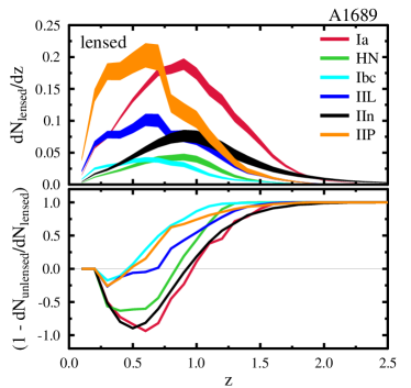
Figure 7: Upper: Redshift distribution for the number of SNe (for each type) assuming the rates estimates by Mannucci et al. (2007) for A1689 in $SZ$-band. Lower: Gain/loss of using A1689 as a lens compared to an equivalent survey without the lens for different redshifts. The crossing of the curves through the zero line indicates the redshift for which a transition to a net gain in SN discoveries is obtained due to the gravitational telescope. An average Milky-Way like extinction with E(B-V)=0.15 was assumed for both plots.

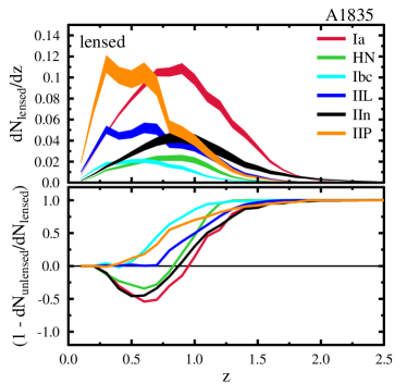
Figure 8: Upper: Redshift distribution of the expected number of SNe (for each type) assuming the rates estimates by Mannucci et al. (2007) for A1835 in $SZ$-band. Lower: Gain/loss of using A1835 as a lens compared to an equivalent survey without the lens for different redshifts. The crossing of the curves through the zero line indicates the redshift for which a transition to a net gain in SN discoveries is obtained due to the gravitational telescope. An average Milky-Way-like extinction with E(B-V)=0.15 was assumed.

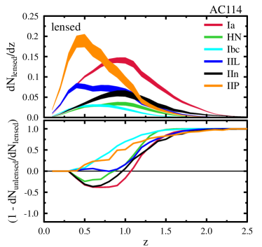
Figure 9: Upper: Redshift distribution of the expected number of SNe (for each type) assuming the rates estimates by Mannucci et al. (2007) for AC114 in $J$-band. Lower: Gain/loss of using AC114 as a lens compared to an equivalent survey without the lens for different redshifts. The crossing of the curves through the zero line indicates the redshift for which a transition to a net gain in SN discoveries is obtained due to the gravitational telescope. An average Milky-Way-like extinction with E(B-V)=0.15 was assumed.

As expected, the boost is most important for the fainter core-collapse supernovae, Type Ib/c and IIP in particular, where the detection efficiency is increased for $z>0.5$. For the brighter SNe, such as Type Ia, it is only for $z>1$ that a net gain is expected. Thus, the foreground massive cluster, besides increasing the flux levels, serves as a high-$z$ filter.

Both AC114 and A1835 (to a somewhat lesser extent) provide comparable total SN rates to A1689 although A1689 is a much stronger lens than the other two clusters. This is because, as already mentioned, the magnification is associated with a shrinkage in the effective volume element.

For simplicity, we restricted this comparison in Figs. 7 to 9 to the volumetric rates estimates in Mannucci et al. (2007). In Fig. 10, the various model predictions for the three clusters combined are shown for each SN type separately.

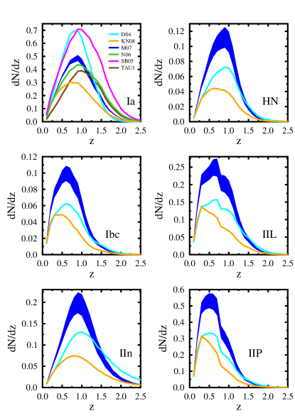
Figure 10: Redshift distribution (including an overall reddening of $E(B-V)=0.15$ and $R_{V}=3.1$) for the number of SNe for the various model predictions for the three clusters combined for each SN type separately.

The expected total number of SNe in our survey is shown in Fig. 11. The estimated rates assume extinction by Galactic-like dust (Cardelli et al., 1989) with an average color excess of $E(B-V)=0.15$ and a total-to-selective extinction coefficient $R_{V}=3.1$, i.e., $A_{V}=0.46$ mag. Since the lensing magnification is typically $\Delta m_{\rm lens}\raise 1.29167pt\hbox{$<$}\kern-7.5pt{\lower 2.79857pt\hbox{$\sim$}}-0.8$, the impact from dust extinction accounts for less than a factor two decrease in the expected number of SN discoveries, compared to the results where dimming by dust is completely neglected.

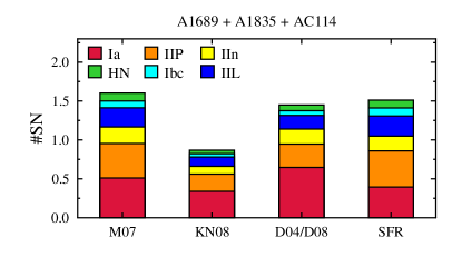
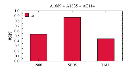
Figure 11: Number of expected SNe for the observations given in Table 3 for (1) the SN rates shown in Figs. 2 and 3, and (2) the SN rates derived from SFR (denoted by SFR) in resolved galaxies described in Sect. 3.2.

6.2 A transient candidate

Paper I described the image subtractions used to search for transient objects in our data set. Transients were sought in both the new images, using archival data as a reference, and for transients in the archival images using the period 79 (April-July 2007) data as a reference. The images were geometrically aligned and the point-spread functions and the flux levels of the two images were matched prior to the pixel subtraction.

In this process, one transient candidate was found in the A1689 archival images in the $SZ$-band. One $I$-band data point of A1689 and two $z$-band data points were observed with FORS2 and another in $J$-band with ISAAC at VLT during the time that the transient was bright. We used HAWK-I $J$-band images from our program in period 81 (July 2008) as a reference to obtain a measurement of the transient flux in that band. Additional reference data from FORS2 and HST/ACS were available for the optical bands. These were used to measure the flux in the region of the transient after it had faded. The transient photometry is summarized in Table 4. The location of the transient and the lensing magnification map is shown in Fig. 12.

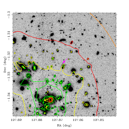
Figure 12: LENSTOOL lensing magnification map of A1689 based on mass model in Limousin et al. (2007) superimposed on top of a HAWK-I $J$-band image from our P81 program (July 2008). The lensing contours for a source at $z=0.6$ for $\Delta m_{\rm lens}$=$(-0.5,-1,-2,-5)$ mag shown in (orange,red,yellow,green). The arrow points to the position of the transient, where a magnification of 1.4$\pm$0.3 mag is expected.

Table 4: Transient candidate photometry from Paper I.

Date	Filter	Magnitude (mag)
2003-02-06	$I$	24.09 $\pm$ 0.20
2003-02-09/10	$z$	23.93 $\pm$ 0.08
2003-02-26/27	$z$	23.94 $\pm$ 0.09
2003-02-09	$SZ$	23.24 $\pm$ 0.08
2003-04-12	$J$	23.61 $\pm$ 0.15
2003-04-27	$SZ$	23.73 $\pm$ 0.16

All available SN templates and a grid of redshifts ($z=[0,3]$) and reddening parameters were tested (allowing for an intrinsic variation in the brightness) and the best fit was found for a Type IIP template based on lightcurves of SN2001cy from Poznanski et al. (2009), redshifted to $z_{\rm SN}=0.59$. Moreover, the best fit of the transient colors was found by assuming that the SN is highly reddened, with a low total-to-selective extinction ratio ($A_{V}$=1.27, $R_{V}$=1.5), as shown in Fig. 13. We note that low values of $R_{V}$, although not seen in the Milky Way, were reported for extinction of quasars (Wang et al., 2004; Östman et al., 2008) and shown to be very common along SN lines of sight (Nobili & Goobar, 2008), possibly as a result of multiple scattering by circumstellar dust (Goobar, 2008). Another possibility is that the intrinsic colors of the SN candidate differ significantly from SN2001cy, in which case a bias could be introduced in the K-corrections. However, a recent study of 40 low-$z$ Type IIP SN lightcurves (Poznanski et al., 2009) found a low average value of the total to selective extinction ratio, $R_{V}=1.5\pm 0.5$, in excellent agreement with the best-fit solution for our SN candidate.

For the nearest galaxy, at $0.5\arcsec$ projected distance, a photometric redshift $z_{\rm gal}=0.60\pm 0.15$ is derived, as shown in Fig. 14. The closest galaxy, $1.2\arcsec$ away, has a photometric redshift that also peaks at $z=0.6$. The distance to the galaxy cores is thus $3.3$ and $7.7$ kpc, respectively.

It should be noted that at $z=0.6$ because of the dust extinction the transient ($J\sim 25$ mag, unlensed) would not have been detected in our survey without the magnification power of the cluster, 1.4 mag. Taking into account the lensing magnification and the assumed host galaxy extinction, we find that the best fit shown in Fig. 13 corresponds to an absolute magnitude $M_{V}=-17.6\pm 0.3$, in good agreement with the assumptions in Table 1. It is striking that the tentative identification of the transient redshift and type match well the expectations for the survey in terms of SN subtype and redshift, as shown in Fig. 7.

We now address the alternative possibility that the transient is at the cluster redshift. A Type Ia supernova more than $70$ days past lightcurve maximum could potentially match the observed brightness of the transient. Sharon et al. (2007) estimated the rate of Type Ia supernovae in intermediate-z clusters to $\sim 0.3$ SNu. For the integrated galaxy luminosity in A1689 of $L_{B}\sim 1.25\cdot 10^{12}L_{\odot}$ and a monitoring time of $\sim 100$ days, about 0.1 Type Ia supernovae were expected in A1689 in our dataset, i.e., a non-negligible possibility. However, as discussed in paper I, the decline rate of SNIa lighturves at late times is 0.01-0.02 mag/day, which is inconsistent with the transient lightcurve.

To conclude, we find that the match to the photometric redshifts of the potential host galaxy and the supernova lightcurves, along with the fitted peak magnitude being consistent with a Type IIP supernova (reddened by dust with $R_{V}$ similar to that found for the nearby sample of Type IIP SNe in (Poznanski et al., 2009)) to represent the most compelling fit to the transient behind A1689.

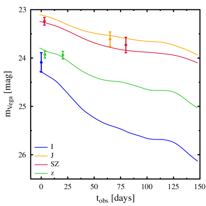
Figure 13: Transient candidate photometry (also listed in Table 4) plotted on top of redshifted ($z_{\rm SN}=0.59$) lightcurves of the very well observed Type IIP SN SN2001cy Poznanski et al. (2009). The nearby SN lightcurves were K-corrected using IIP spectral templates derived from spectra and photometry of SN2001cy and reddened following the extinction law in Fitzpatrick (1999) with the parameters $E(B-V)=0.85$ and $R_{V}=1.5$ yielding $\chi^{2}=3.5$ for 6 data points and 4 free parameters.

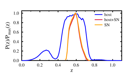
Figure 14: Probability distribution function for the photometric redshift (seven bands) of the galaxy closest (0.5 arcseconds) to the transient, the SN photo-$z$ assuming a IIP template matching SN2001cy and the product of the two, yielding $z=0.59\pm 0.05$.

7 Implications for future near-IR surveys

The pilot survey was completed with the ISAAC instrument at VLT, which has a FOV of 2.5’$\times$2.5’ and a threshold of $\sim$24 mag (Vega) for $SZ$ and $J$-bands and relatively few observations. We briefly discuss the feasibility of building up lightcurves of lensed SNe behind clusters of galaxies for surveys with 8-meter class ground-based telescopes and large FOV near-IR instruments, such as HAWK-I at VLT or MOIRCS at Subaru. We consider a five-year “rolling” search survey, with imaging spaced at intrevals of 30 days.

The lensing model of A1689 is used as our baseline for estimating the number of SNe behind a massive cluster as a function of redshift. Thus, the results below apply to the most massive clusters, $M\sim 10^{15}M_{\odot}$. We also consider a survey period of five years since this is optimal for the discovery of multiple images (Sect. 7.1). In practice, several clusters would have to be observed to correspond to ’five A1689 years’ since that particular field is behind the Sun part of the year.

During period 81 (P81, July 2008), our team started a survey targeting lensed SNe behind A1689 using the increased sensitivity and FOV ($\approx$ 7.5’$\times$7.5’) of HAWK-I on VLT. The limited availability of the instrument in P81, only a few, closely spaced observations were completed. Although the observations were not suited to transient searches, the dataset could be used to estimate the depth of the point-source search in $J$-band that was continued during P82 (early 2009) to $\sim 24.65$ mag (Vega) for 90% detection efficiency, i.e., about 0.65 mag deeper than the survey done with ISAAC.

We now examine the feasibility of SN detection with HAWK-I. We use LENSTOOL to calculate the lensing magnification map of A1689 for the larger FOV. Although the magnification decreases with distance from the cluster core, reaching $\Delta m_{\rm lens}\sim-0.25$ at the edges of the FOV, the impact of lensing remains very important for detecting distant supernovae. In the upper panel of Fig. 15, the differential number of SNe is shown for the various types of SNe. The lower part of the figure shows the gain and loss of lensing compared to the same survey without lensing as a function of redshift. As expected, fewer SNe are found at low redshifts, while the survey depth is significantly increased. The integrated number of SNe for the various models is shown in Fig. 16.

For HAWK-I (and the A1689 mass model), we expect on the order of 40-70 SNe (depending on the underlying rate estimate for the various SN types) of which about a dozen will be at $z>1.5$. In Fig. 17, the potential of the suggested rolling search for generating lensed supernova lightcurves in the redshift range $(1<z<2)$ is shown. The repeated images are used both to discover new supernovae and to build up lightcurves for earlier discoveries. The supernova types and redshift distribution matches the differential rates in Fig. 15.

Surveys for lensed supernovae with space instruments would complementthe ground-based approaches since even higher redshifts could be reached due to the deeper point source sensitivity.

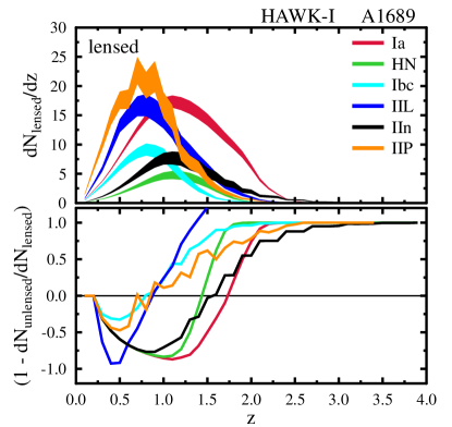
Figure 15: Upper: Redshift distribution of SN discoveries in a 5-year survey behind a very massive cluster (model of A1689 used). Lower: Gain/loss of using a A1689-like cluster as a lens compared to an equivalent survey without the lens for different redshifts. The crossing of the curves through the zero line indicates the redshift for which a transition to a net gain in SN discoveries is obtained due to the gravitational telescope. An average Milky-Way-like extinction with $E(B-V)=0.15$ was assumed together with SN rates from M07.

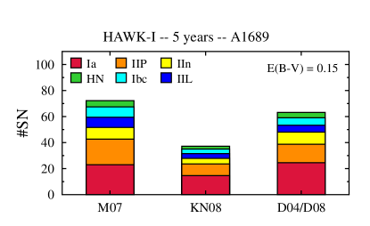
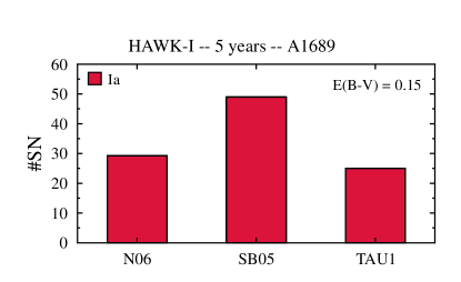
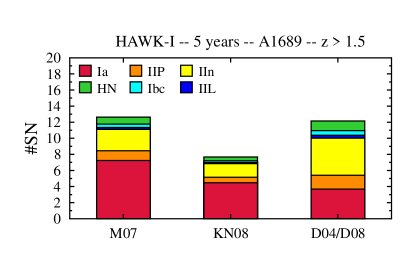
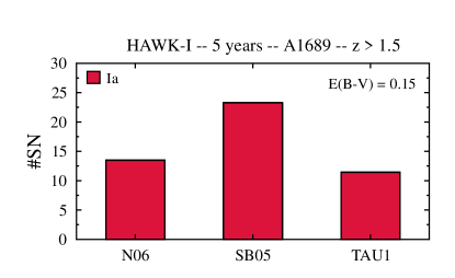
Figure 16: (Top) Number of SNe expected in a 5 year monthly survey of one very massive, A1689-like cluster, with HAWK-I. (Bottom) Number of SNe with $z>1.5$.

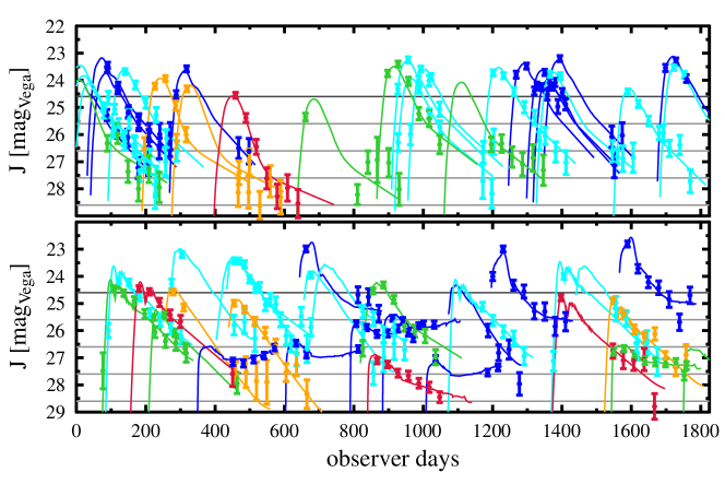
Figure 17: Simulated lightcurve sampling for supernovae in the redshift range $1<z<2$ in a 5-year monthly survey of A1689 and AC114 with HAWK-I. The top panel shows the expected lightcurves sampling SNIa. Core-collapse SNe are shown in the bottom panel. The vertical axis shows the unlensed magnitudes. The symbol colors indicate the SN redshift: blue ($z=[1.0,1.2]$), cyan ($z=[1.2,1.4]$), green ($z=[1.4,1.6]$), orange ($z=[1.6,1.8]$), and red ($z=[1.8,2.0]$).

7.1 Multiple SN images

When looking through a gravitational lens, multiple images of the same source image can be observed. This is also true for SNe that, due to strong lensing, can potentially be detected to very high redshifts. About one in a hundred SNe behind A1689 in the HAWK-I FOV would have multiple images with time separations of between weeks and a few years. Thus, about 0.5-1.0 SNe with multiple images are expected in a 5 year survey with HAWK-I.

Figure 18 indicates the fraction of the source areas with multiply lensed SNe that can be observed as a function of survey time for two different redshifts. For $z=1$, all SN types show the same behavior and given a sufficiently large survey time, at least two (or more) images of the SN could be observed, regardless of its type. At higher redshifts ($z=2$), given a sufficiently large survey time, most of the brighter SNe (Ia and IIn) and about half of the IIL_bright and HN will be observable and have at least two (or more) images. The other SN types (IIL, Ib/c, and IIP) will be too faint – even with magnification – to be observed. For all considered redshifts, a 5 year survey (or longer) is optimal for discovering multiple images of SNe behind clusters.

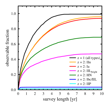
Figure 18: Fraction of SNe with multiple images that are observable as a function of survey duration.

Detecting these rare events could provide important constraints on the Hubble constant with the time-delay technique (Refsdal, 1964) as well testing dark matter and energy properties in an unexplored redshift range (Goobar et al., 2002; Mörtsell & Sunesson, 2006). Models of lens systems are in general uncertain due to the possibility to rescale the density distribution of the lens and add a circularly symmetric density mass-sheet, while preserving the observed image configuration (Gorenstein et al., 1988; Liesenborgs et al., 2008). This mass-sheet degeneracy can be broken if the absolute magnification of the lens is known. Since SNIa have a very tight dispersion in brightness, these lens systems would constitute an ideal sample for minimizing three major systematic uncertainties in the estimates of $H_{0}$ using the time-delay technique: accurate time estimates from supernova lightcurves, elimination of the mass-sheet degeneracy, and accurate lens models because of the large number of lensed background galaxies, as discussed in Paper III.

8 Conclusions

Powerful gravitational telescopes in the form of massive galaxy clusters provide unique opportunities to discover transient objects such as SNe at redshifts beyond what can be reached with current telescopes. The lensing magnification $\mu$ corresponds to a gain factor in exposure length, $\mu^{2}$, while at the same time the solid angle at the source planes shrinks by a factor $\mu$ for source redshifts higher than the cluster redshift. The net gain/loss of searching for supernovae behind massive clusters is therefore a non-trivial combination of FOV, limiting depth, and supernova luminosity functions. In general, the lens works as a magnifying glass and high-$z$ filter, i.e., by reducing the number of detections of bright/close supernovae and enhancing the detections of distant/faint objects. Thus, to be successful, a SN survey behind galaxy clusters needs to be optimized. Clearly, for extremely sensitive (e.g JWST or ELT) or very large FOV instruments, the positive impact of the lensing cluster may be negligible, at least for the brightest types of supernovae. The net benefit of exploiting the suggested approach will ultimately depend on the rate and intrinsic brightness of the various types of SNe at redshifts beyond what is currently known. For Type Ia supernovae, an important parameter determining the rates beyond $z=1.5$ is the delay time, $\tau$. By increasing the redshift sensitivity beyond that achieved by “standard” surveys, we may significantly improve our understanding of SNIa progenitors. Similarly, little is known about the dimming of supernovae by dust at very high redshifts. The combination of a longer wavelength-survey and higher sensitivity to fainter high-$z$ SNe could thus lead to detections of a different population of objects.

A combined 40-hour dataset involving archival ISAAC data and new observations obtained in 2007 for three very massive clusters (A1689, A1835, and AC114) was used to determine the feasibility of discovering lensed core-collapse and Type Ia SNe. Considering the monitoring time available, the area surveyed, the lensing magnification, and the survey magnitud limit, rate estimates of the various SN subtypes considered were calculated. Synthetic lightcurves of SNe and several models of the volumetric Type Ia and core-collapse SN rates as a function of redshift were used, all consistently predicting a Poisson mean value for the expected number of SNe in the survey of between N_SN=0.8 and 1.6 for all SNe. One transient object was found behind A1689 on a galaxy with photometric redshift $z_{\rm gal}=0.6\pm 0.15$, the most probable redshift for SN detection in the ISAAC/VLT survey. The lightcurve is consistent with being a reddened Type IIP supernova at $z_{\rm SN}=0.59\pm 0.05$. At the position and redshift of the transient, the lensing model predicts $1.4$ magnitudes of magnification.

Because of the recent deployment of large and sensitive near-IR cameras, such as HAWK-I at VLT, the search for the highest redshift SNe can now be moved to longer wavelengths, thus avoiding the difficulties involved with restframe UV observations, and extending the potential for supernova discoveries, especially Type Ia supernovae, beyond $z>2$. A feasibility study of the potential to build up lightcurves of lensed SNe with larger and deeper surveys shows that this is a very exciting path for new discoveries. The equivalent of a five-year monthly survey of a single very massive cluster with the HAWK-I camera at VLT would yield $40-70$ lensed SNe, most of them with good lightcurve sampling. Thus, a dedicated multi-year NIR rolling search targeting several massive clusters would lead to a high rate of very high-$z$ SN discoveries, thus making this approach complementary to deep optical space-based SN surveys (Riess et al., 2007) as well large field-of-view optical SN searches, e.g., (Poznanski et al., 2007).

Although very rare, multiple images of strongly lensed SNe are within reach of such a survey and could offer potentially exciting tests of cosmological parameters as well as improvements to the cluster mass modeling.

References

- Astier et al. (2006) Astier, P. et al. 2006, A&A, 447, 31
- Broadhurst et al. (2005) Broadhurst, T. et al. 2005, ApJ, 621, 53
- Campusano et al. (2001) Campusano, L. E., Pelló, R., Kneib, J.-P., Le Borgne, J.-F., Fort, B., Ellis, R., Mellier, Y., & Smail, I. 2001, A&A, 378, 394
- Cardelli et al. (1989) Cardelli, J. A., Clayton, G. C., & Mathis, J. S. 1989, ApJ, 345, 245
- Chary & Elbaz (2001) Chary, R., & Elbaz, D. 2001, ApJ, 556, 562
- Dahlen et al. (2007) Dahlen, T., Mobasher, B., Dickinson, M., Ferguson, H. C., Giavalisco, M., Kretchmer, C., & Ravindranath, S. 2007, ApJ, 654, 172
- Dahlen et al. (2005) Dahlen, T., Mobasher, B., Somerville, R. S., Moustakas, L. A., Dickinson, M., Ferguson, H. C., & Giavalisco, M. 2005, ApJ, 631, 126
- Dahlen et al. (2008) Dahlen, T., Strolger, L.-G., & Riess, A. G. 2008, ApJ, 681, 462
- Dahlen et al. (2004) Dahlen, T. et al. 2004, ApJ, 613, 189
- Filippenko (1997) Filippenko, A. V. 1997, ARA&A, 35, 309
- Fitzpatrick (1999) Fitzpatrick, E. L. 1999, PASP, 111, 63
- Frieman et al. (2008) Frieman, J. A. et al. 2008, AJ, 135, 338
- Gal-Yam et al. (2002) Gal-Yam, A., Maoz, D., & Sharon, K. 2002, MNRAS, 332, 37
- Giavalisco et al. (2004) Giavalisco, M. et al. 2004, ApJ, 600, L103
- Gnedin et al. (2008) Gnedin, N. Y., Kravtsov, A. V., & Chen, H.-W. 2008, ApJ, 672, 765
- Goobar (2008) Goobar, A. 2008, ApJ, 686, L103
- Goobar et al. (2002) Goobar, A., Mörtsell, E., Amanullah, R., & Nugent, P. 2002, A&A, 393, 25
- Gorenstein et al. (1988) Gorenstein, M. V., Shapiro, I. I., & Falco, E. E. 1988, ApJ, 327, 693
- Gunnarsson & Goobar (2003) Gunnarsson, C., & Goobar, A. 2003, A&A, 405, 859
- Gwyn (1995) Gwyn, S. D. J. 1995, Master’s thesis, MS Thesis, University of Victoria (1995)
- Hopkins & Beacom (2006) Hopkins, A. M., & Beacom, J. F. 2006, ApJ, 651, 142
- Jullo et al. (2007) Jullo, E., Kneib, J.-P., Limousin, M., Elíasdóttir, Á., Marshall, P. J., & Verdugo, T. 2007, New Journal of Physics, 9, 447
- Kim et al. (1996) Kim, A., Goobar, A., & Perlmutter, S. 1996, PASP, 108, 190
- Kneib et al. (2004) Kneib, J.-P., Ellis, R. S., Santos, M. R., & Richard, J. 2004, ApJ, 607, 697
- Kneib et al. (1996) Kneib, J.-P., Ellis, R. S., Smail, I., Couch, W. J., & Sharples, R. M. 1996, ApJ, 471, 643
- Kobayashi & Nomoto (2008) Kobayashi, C., & Nomoto, K. 2008, ArXiv:0801.0215
- Kobayashi et al. (1998) Kobayashi, C., Tsujimoto, T., Nomoto, K., Hachisu, I., & Kato, M. 1998, ApJ, 503, L155+
- Kolatt & Bartelmann (1998) Kolatt, T. S., & Bartelmann, M. 1998, MNRAS, 296, 763
- Kovner & Paczynski (1988) Kovner, I., & Paczynski, B. 1988, ApJ, 335, L9
- Kuznetsova et al. (2008) Kuznetsova, N. et al. 2008, ApJ, 673, 981
- Leibundgut (2008) Leibundgut, B. 2008, General Relativity and Gravitation, 40, 221
- Lien & Fields (2009) Lien, A., & Fields, B. D. 2009, Journal of Cosmology and Astro-Particle Physics, 1, 47
- Liesenborgs et al. (2008) Liesenborgs, J., de Rijcke, S., Dejonghe, H., & Bekaert, P. 2008, MNRAS, 386, 307
- Limousin et al. (2007) Limousin, M. et al. 2007, ApJ, 668, 643
- Mannucci et al. (2007) Mannucci, F., Della Valle, M., & Panagia, N. 2007, MNRAS, 377, 1229
- Mannucci et al. (2005) Mannucci, F., Della Valle, M., Panagia, N., Cappellaro, E., Cresci, G., Maiolino, R., Petrosian, A., & Turatto, M. 2005, A&A, 433, 807
- Miknaitis et al. (2007) Miknaitis, G. et al. 2007, ApJ, 666, 674
- Mobasher et al. (1996) Mobasher, B., Rowan-Robinson, M., Georgakakis, A., & Eaton, N. 1996, MNRAS, 282, L7
- Mörtsell & Sunesson (2006) Mörtsell, E., & Sunesson, C. 2006, Journal of Cosmology and Astro-Particle Physics, 1, 12
- Neill et al. (2006) Neill, J. D. et al. 2006, AJ, 132, 1126
- Nobili & Goobar (2008) Nobili, S., & Goobar, A. 2008, A&A, 487, 19
- Östman et al. (2008) Östman, L., Goobar, A., & Mörtsell, E. 2008, A&A, 485, 403
- Poznanski et al. (2009) Poznanski, D. et al. 2009, ApJ, 694, 1067
- Poznanski et al. (2007) ——. 2007, MNRAS, 382, 1169
- Pritchet et al. (2008) Pritchet, C. J., Howell, D. A., & Sullivan, M. 2008, ApJ, 683, L25
- Refsdal (1964) Refsdal, S. 1964, MNRAS, 128, 307
- Richard et al. (2006) Richard, J., Pelló, R., Schaerer, D., Le Borgne, J.-F., & Kneib, J.-P. 2006, A&A, 456, 861
- Richardson et al. (2002) Richardson, D., Branch, D., Casebeer, D., Millard, J., Thomas, R. C., & Baron, E. 2002, AJ, 123, 745
- Riess et al. (2007) Riess, A. G. et al. 2007, ApJ, 659, 98
- Salpeter (1955) Salpeter, E. E. 1955, ApJ, 121, 161
- Scannapieco & Bildsten (2005) Scannapieco, E., & Bildsten, L. 2005, ApJ, 629, L85
- Seitz et al. (1998) Seitz, S., Saglia, R. P., Bender, R., Hopp, U., Belloni, P., & Ziegler, B. 1998, MNRAS, 298, 945
- Sharon et al. (2007) Sharon, K., Gal-Yam, A., Maoz, D., Filippenko, A. V., & Guhathakurta, P. 2007, ApJ, 660, 1165
- Smartt et al. (2009) Smartt, S. J., Eldridge, J. J., Crockett, R. M., & Maund, J. R. 2009, MNRAS, 395, 1409
- Stanishev et al. (2009) Stanishev, V. et al. 2009, ArXiv e-prints, 0908.4176
- Strolger et al. (2004) Strolger, L.-G. et al. 2004, ApJ, 613, 200
- Sullivan et al. (2000) Sullivan, M., Ellis, R., Nugent, P., Smail, I., & Madau, P. 2000, MNRAS, 319, 549
- Sullivan et al. (2006) Sullivan, M. et al. 2006, ApJ, 648, 868
- Wang et al. (2004) Wang, J., Hall, P. B., Ge, J., Li, A., & Schneider, D. P. 2004, ApJ, 609, 589