Partition Function of Spacetime

Abstract

We consider a microscopic model of spacetime, where spacetime is assumed to be a specific graph with Planck size quantum black holes on its vertices. As a thermodynamical system under consideration we take a certain uniformly accelerating, spacelike two-surface of spacetime which we call, for the sake of brevity and simplicity, as acceleration surface. Using our model we manage to obtain an explicit and surprisingly simple expression for the partition function of an acceleration surface. Our partition function implies, among other things, the Unruh and the Hawking effects. It turns out that the Unruh and the Hawking effects are consequences of a specific phase transition, which takes place in spacetime, when the temperature of spacetime equals, from the point of view of an observer at rest with respect to an acceleration surface, to the Unruh temperature measured by that observer. When constructing the partition function of an acceleration surface we are forced to introduce a quantity which plays the role of thermal energy of the surface. An interpretation of that quantity as energy in a normal manner yields Einstein’s field equation with a vanishing cosmological constant for general matter fields.

I Introduction

Is spacetime made of some elementary constituents in the same way as matter is made of atoms? This is one of the central questions of the so called emergent gravity, which views gravity as an emergent, instead of a fundamental property of spacetime. According to some ideas of emergent gravity, which have gained increasing popularity during some recent years, gravitation appears at macroscopic length scales as a consequence of the properties of a some still unknown substructure of spacetime in the same way as, say, an elasticity of a solid body is a consequence of the properties of its atoms. yksi If the aims of emergent gravity were realized, one should be able to obtain all of the ”hard facts” of gravity as such as we know them today, together with some possible new predictions, from an appropriate microscopic model of spacetime. Those hard facts include, among other things, Einstein’s classical general relativity with all of its consequences, together with the Unruh and the Hawking effects. An ability to predict general relativity, as well as the Unruh and the Hawking effects, at macroscopic length scales acts as a crucial test for any viable microscopic model of spacetime.

When one goes over from a microscopic to a macroscopic description of any system, the key role is played by the partition function

$$Z(\beta):=\sum_{n}g(E_{n})e^{-\beta E_{n}}$$ (1)

of the system. If we know the partition function of a system, we may calculate the macroscopic quantities relevant to the system as functions of its inverse temperature $\beta$ in a very simple manner. For instance, the average total energy of the system is

$$E(\beta)=-\frac{\partial}{\partial\beta}\ln Z(\beta),$$ (2)

and its entropy is, in natural units:

$$S(\beta)=\beta E(\beta)+\ln Z(\beta).$$ (3)

In Eq.(1.1) $E_{n}$ denotes the possible energy eigenvalues of a system, and $g(E_{n})$ is the number of degenerate states corresponding to the same energy eigenvalue $E_{n}$. When one attempts to obtain the macroscopic propeties of gravity from an appropriate microscopic model of spacetime, one must first calculate the partition function of spacetime. The properties of the partition function should then imply the properties of gravity at macroscopic length scales.

In this paper we consider a specific microscopic model of spacetime. Using our model we manage to obtain an explicit - and surprisingly simple - expression for the partition function of spacetime. Our partition function implies, among other things, the Hawking and the Unruh effects, together with a formula very similar to the Bekenstein-Hawking entropy law for black holes. According to our model the Hawking and the Unruh effects are consequences of a certain type of phase transition, which takes place in spacetime. During this phase transition the fundamental constituents of spacetime jump from a one quantum state to another in a very specific way. When calculating the partition function we are forced to introduce a concept, which plays the role of thermal energy in our model. An interpretation of that concept as energy in a normal manner implies Einstein’s field equation with a vanishing cosmological constant.

This paper is a continuation to a series of papers, where Planck size quantum black holes were used as the fundamental constituents of spacetime. kaksi ; kolme ; nelja As in those papers, we model spacetime by a specific graph, where black holes lie on the vertices. The only physical degree of freedom associated with an individual black hole is its event horizon area, which is assumed to have a discrete spectrum with an equal spacing. More precisely, the eigenvalues of the event horizon area are assumed to be of the form

$$A_{n}=(n+\frac{1}{2})32\pi\ell_{Pl}^{2},$$ (4)

where $n=0,1,2,...$, and

$$\ell_{Pl}:=\sqrt{\frac{\hbar G}{c^{3}}}\approx 1.6\times 10^{-35}m$$ (5)

is the Planck length. A horizon area spectrum with an equal spacing for black holes was proposed by Bekenstein already in 1974. viisi Since then Bekenstein’s proposal has been recovered by several authors on various grounds, and it has been an object of wide and detailed investigations. kuusi One of the key ideas of our model of spacetime is to reduce all properties of spacetime to the horizon area eigenstates of the Planck size quantum black holes constituting spacetime. kaksi

There are some indications that at the Planck scale of distances microscopic black holes might really play some role in the structure of spacetime. For instance, if we close a particle inside a box with an edge length equal to the Planck length $\ell_{Pl}$, then Heisenberg’s uncertainty principle implies that the momentum of the particle has an uncertainty $\Delta p\sim\hbar/\ell_{Pl}$. In the ultrarelativistic limit the uncertainty $\Delta p$ in the momentum corresponds to the uncertainty $\Delta E\sim c\Delta p$ in the energy of the particle. In other words, inside a box with edge length equal to $\ell_{Pl}$ we have closed a particle, which has the Planck energy

$$E_{Pl}:=\sqrt{\frac{\hbar c^{5}}{G}}\approx 2.0\times 10^{9}J$$ (6)

as an uncertainty in its energy. This energy, however, is enough to shrink the box into a black hole with a Schwarzschild radius equal to about one Planck length. So it seems that when probing spacetime at the Planck scale of distances one is likely to meet with Planck size black holes.

The idea that spacetime might consist of tiny black holes is far from new. Somewhat related ideas have been expressed, for instance, by Misner, Thorne and Wheeler in their book. seitseman Unfortunately, the idea of spacetime being made of Planck size black holes has never been taken very far. This paper is a part of an ongoing project, where this idea is being explored systematically.

The very first question one should always ask at the beginning of an investigation of a physical problem is: ”What is the system under consideration?” For a solid state physicist, for instance, the system may be a piece of metal, and he may be interested to explain its macroscopic properties, such as specific heat and electric conductivity, by means of the properties of its atoms, whereas an elementary particle physicist, in turn, may be interested in a system which consists of two elementary particles, and a particle which intermediates their mutual interactions.

In this paper we propose that the system one should consider in gravitational physics at the macroscopic length scales is the so called acceleration surface which was introduced in Ref. kolme . To put it simply, an acceleration surface may be described as a smooth, orientable, simply connected, spacelike two-surface of spacetime, whose every point accelerates uniformly with a constant proper acceleration to the direction of a spacelike unit normal vector field of the surface. Examples of acceleration surfaces include, among other things, a uniformly accelerating spacelike plane in flat Minkowski spacetime, and the $t=constant$ slices of a timelike hypersurface, where $r=constant$ $(>2M)$ in Schwarzschild spacetime equipped with the Schwarzschild coordinates. In our model acceleration surfaces are assumed to be made of Planck size quantum black holes in a somewhat similar way as solids are made of atoms, and from the postulated properties of those black holes we infer the macroscopic properties of acceleration surfaces.

A detailed investigation of the geometrical and the dynamical properties of acceleration surfaces was performed in Ref. kolme . To make our presentation self-contained, we begin our considerations, in Section 2, by an extensive review of those properties. One of the motivations for introducing the concept of acceleration surface is Jacobson’s remarkable discovery of the year 1995 that Einstein’s field equation may be obtained from the thermodynamical relation $\delta Q=T\,dS$ and certain assumptions concerning the properties of the local past Rindler horizon of an accelerating observer. kahdeksan More precisely, Jacobson assumed that when matter flows through of a finite part of the horizon, that part shrinks such that the entropy carried by the matter through the horizon is, in natural units, exactly one-quarter of the decrease in the area of that part. In other words, Jacobson managed to show that Einstein’s field equation may be obtained from certain thermodynamical assumptions concerning the properties of Rindler horizons. Acceleration surfaces may be viewed as generalizations of the horizons of spacetime in the sense that an arbitrary horizon of spacetime is always a limit of a certain acceleration surface, if we take the proper acceleration $a$ of that surface to infinity. One of the key questions is, whether Jacobson’s thermodynamical derivation of Einstein’s field equation may be extended for surfaces more general than Rindler horizons, and acceleration surfaces provide an appropriate generalization.

In Section 2 we present a mathematically precise definition of the concept of acceleration surface. When an acceleration surface propagates in spacetime, its area may change, and we write the equations, exactly derived in Ref. kolme , which tell how the changes in the area of an acceleration surface depend on the geometry of the underlying spacetime. A question of fundamental importance is, whether it is possible to associate a quantity analogous to thermal energy with acceleration surfaces in any physically meaningful way. Motivated by the analogies drawn from Newtonian gravity, Unruh effect, and the mass formula of black holes we argue that this is indeed possible. Additional motivation for defining the concept of thermal energy, or heat, for an acceleration surface in a certain manner is provided by the fact that Einstein’s field equation with a vanishing cosmological constant may be obtained from a very simple equation which describes the exchange of heat between an acceleration surface and massless, non-interacting radiation flowing through that surface. Since that equation really implies, as we show in Section 2, Einstein’s field equation with a vanishing cosmological constant, not only for radiation, but for general matter fields, we call that equation, in our model, as the ”fundamental equation” of the thermodynamics of spacetime. The derivation of Einstein’s field equation from our fundamental equation provides a generalization of Jacobson’s thermodynamical derivation.

In Section 3 we proceed from the macroscopic and classical description of acceleration surfaces performed in Section 2 to their microscopic and quantum-mechanical description. We pose four independence- and two statistical postulates for the black holes constituting the acceleration surfaces of spacetime. The independence postulates imply, among other things, that the possible eigenvalues of the area $A$ of an acceleration surface are of the form:

$$A=\alpha\ell_{Pl}^{2}(n_{1}+n_{2}+...+n_{N}),$$ (7)

where $\alpha$ is a pure number of the order of unity, and the non-negative integers $n_{1},n_{2},...,n_{N}$ are the quantum numbers labelling the horizon area eigenstates of the $N$ individual black holes which constitute the surface. The statistical postulates, in turn, identify the microscopic and the macroscopic states of an acceleration surface. The microscopic states of an acceleration surface are determined by the different combinations of the non-vacuum ($n\neq 0$) horizon area eigenstates of the quantum black holes on the surface, and each microscopic state yielding the same area eigenvalue of the surface corresponds to the same macroscpic state. When writing the partition function of an acceleration surface we identify the energy of the surface as the thermal energy defined in Section 2. Our definition implies that there is a one-to-one relationship between the area- and the energy eigenvalues of a given acceleration surface, and therefore the number $g(E_{n})$ of the degenerate states corresponding to the same energy eigenvalue $E_{n}$ of the surface equals to the number of microstates corresponding to the same area $A$. Hence the calculation of the degeneracy $g(E_{n})$ becomes to an easy excercise of combinatorics: Basically, the calculation of $g(E_{n})$ boils down to the question of in how many ways a given positive integer $n$ may be expressed as a sum of at most $N$ positive integers.

After finding the allowed values of $E_{n}$ and the corresponding values of $g(E_{n})$ it is easy to write the partition function of an acceleration surface. An actual calculation of the partition function, however, is rather involved, and the details of that calculation have been expressed in the Appendix A of this paper. Nevertheless, the calculation may be carried out explicitly, and the final result turns out to be miraculously simple. The partition function of an acceleration surface consisting of $N$ Planck size quantum black holes is, in natural units:

$$Z(\beta)=\frac{1}{2^{\beta T_{C}}-2}\biggl{[}1-\biggl{(}\frac{1}{2^{\beta T_{C}}-1}\biggr{)}^{N+1}\biggr{]}.$$ (8)

In this equation

$$T_{C}:=\frac{\alpha\hbar a}{4(\ln 2)\pi k_{B}c},$$ (9)

and we call $T_{C}$ as the characteristic temperature of an acceleration surface with a proper acceleration $a$. Eq.(1.8) holds, whenever $\beta T_{C}\neq 1$. If $\beta T_{C}=1$, we have $Z(\beta)=N+1$.

In Sections 4 and 5 we work out the consequences of Eq.(1.8). In Section 4 we consider the dependence of the energy $E$ of an acceleration surface on its absolute temperature $T$. It turns out that the characteristic temperature $T_{C}$ plays an important role: If $T<T_{C}$, the energy $E$ is, for large $N$, effectively zero, which means that all quantum black holes on an acceleration surface are in vacuum. However, when $T=T_{C}$, the acceleration surface performs a phase transition, where the energy of the surface increases, although its temperature remains the same. During this phase transition the black holes constituting an acceleration surface jump, in average, from the vacuum to the second excited states. We have investigated this phase transition both analytically and numerically. When $T>T_{C}$, the energy of an acceleration surface depends, in effect, linearly on its absolute temperature $T$.

Because the energy of an acceleration surface is effectively zero, when the temperature $T$ measured by an observer for the surface is less than its characteristic temperature $T_{C}$, one may view the temperature $T_{C}$ as the lowest possible temperature which an accelerated observer may measure; otherwise all black holes on the surface would be in vacuum. So we find that our model predicts the Unruh effect. According to the Unruh effect the Unruh temperature $T_{U}:=\frac{a}{2\pi}$ is the lowest possible temperature which an accelerated observer may measure in the sense that $T_{U}$ is the characteristic temperature of the thermal radiation detected by an accelerated observer even when all matter fields are, from the point of view of all inertial observers, in vacuum. yhdeksan It is a common feature of the temperatures $T_{C}$ and $T_{U}$ that they are both proportional to the proper acceleration $a$ of the observer. If we identify the temperatures $T_{C}$ and $T_{U}$ we may fix the undetermined number $\alpha$ in Eqs.(1.7) and (1.9). We get:

$$\alpha=2\ln 2.$$ (10)

In addition of predicting the Unruh effect, our model also predicts the Hawking effect, which we show explicitly for Schwarzschild black holes in Section 4. More precisely, we show that we may take an appropriate acceleration surface arbitrarily close to the Schwarzschild horizon of a Schwarzschild black hole, and the temperature measured by an observer at rest on that surface is exactly the Hawking temperature measured by an observer just outside of the horizon.

Section 5 is dedicated to the investigation of the entropic properties of acceleration surfaces. One finds that for an acceleration surface area $A$ there is a certain critical value $A_{crit}$, which corresponds to the situation, where all black holes on the surface are, in average, on the second excited state. If $A<A_{crit}$, the temperature of the surface is $T_{C}=T_{U}$ to a very great precision and the entropy $S$ of the surface is, for large $N$, directly proportional to $A$. More precisely, the entropy $S$ is, in natural units, exactly one-half of the area, when $N$ goes to infinity. In other words, one gains for the acceleration surface entropy a value which is exactly twice the Bekenstein-Hawking entropy of a black hole with the same event horizon area. kymmenen ; yksitoista This result is in harmony with the findings of Refs. kaksitoista ; kolmetoista ; neljatoista . When $A>A_{crit}$, however, one finds for the entropy $S$ an expression:

$$S(A)=\frac{1}{2\ln 2}\frac{k_{B}c^{3}}{\hbar G}A\ln(\frac{2A}{2A-A_{crit}})+Nk_{B}\ln(\frac{2A-A_{crit}}{A_{crit}}).$$ (11)

As one may observe, this expression contains logarithms of the area $A$.

We close our dicussion in Section 6 with some concluding remarks. Unless otherwise stated, we shall always use the natural units, where $\hbar=G=c=k_{B}=1$.

II Preliminaries: Acceleration Surfaces and Their Properties

II.1 The Concept of Acceleration Surface

During some recent years there has been accumulating evidence that general relativity may be understood in terms of the properties of certain spacelike two-surfaces of spacetime. One of the first steps in this direction was taken by Jacobson already in 1995, when he managed to show that Einstein’s field equation may be obtained from the first law of thermodynamics and an assumption that any finite part of the past Rindler horizon of an accelerating observer possesses, in a certain sense, an amount of entropy which, in the natural units, is exactly one-quarter of the area of that part. kahdeksan More precisely, Jacobson considered the flow of matter through the past Rindler horizon of an accelerating observer, and he identified the boost energy flow of the matter through the horizon as its heat flow. Assuming that the horizon shrinks during the flow of matter through the horizon such that the amount of entropy carried by the matter through the horizon is, when the temperature of the matter equals with the Unruh temperature of the observer, exactly one-quarter of the decrease in the horizon area, Jacobson found that Einstein’s field equation is a straightforward consequence of the first law of thermodynamics. Somewhat related investigations have been made by Padmanabhan and his collaborators. viisitoista They have found that Einstein’s field equation may be obtained by varying the boundary term in the Einstein-Hilbert action, when the boundary consists of a horizon of spacetime.

A horizon of spacetime is a certain null hypersurface, and it is created, when the points of an appropriate spacelike two-surface move along certain null curves of spacetime. A Rindler horizon in Minkowski spacetime equipped with the flat Minkowski metric, for instance, consists of the world lines of the points of the plane with $x\equiv 0$ for $t=0$, when the points of that plane move along the null lines, where $x=\pm t$, and the coordinates $y$ and $z$ of the points are constants. One may therefore wonder, whether Einstein’s field equation could as well be obtained from the properties of a spacelike two-surface whose points move along curves different from the null curves of spacetime. In other words, is it really necessary to restrict the considerations to the horizons of spacetime?

There really exist spacelike two-surfaces which are not parts of any horizons of spacetime in the sense described above, and whose dynamical properties nevertheless imply Einstein’s field equation. A specific example of this kind of a surface is the so called acceleration surface. In broad terms, acceleration surface may be described as a smooth, orientable, simply connnected, spacelike two-surface of spacetime, whose every point is accelerated with a constant proper acceleration $a$ to the direction of a spacelike unit normal $n^{\mu}$ of the surface. For instance, a flat plane parallel to the $xy$-plane and accelerating, in the rest frame of the plane, with a constant proper acceleration to the direction of the $z$-axis in flat Minkowski spacetime provides a simple example of an acceleration surface. A mathematically precise definition of acceleration surface is pretty involved, and it deals with the properties of the proper acceleration vector field

$$a^{\mu}:=u^{\alpha}u^{\mu}_{;\alpha}$$ (12)

of a certain smooth congrunce of certain timelike curves. For the sake of brevity and simplicity we shall call the congruence in question as acceleration congruence. In Eq.(2.1) the semicolon denotes the covariant derivative, and $u^{\mu}$ is the future directed unit tangent vector field of the congruence.

To be quite precise, acceleration congruence is defined as a smooth congruence of future directed timelike curves parametrized by the proper time $\tau$ measured along these curves such that:

(i) All those sets of points, where $\tau=constant$ along the elements of the congruence are smooth, orientable, spacelike two-surfaces of spacetime.

(ii) The norm, or absolute value

$$||a^{\mu}||:=\sqrt{a^{\mu}a_{\mu}}:=a$$ (13)

of the proper acceleration vector field $a^{\mu}$ of the congruence is identically constant.

(iii) For arbitrary, fixed $\tau$ the proper acceleration vector field $a^{\mu}$ is parallel to a spacelike unit normal vector field $n^{\mu}$ of the spacelike two-surface, where $\tau=constant$.

(iv) The spacelike two-surface, where $\tau=0$, intersects orthogonally the elements of the congruence.

After defining the concept of acceleration congruence we may define acceleration surface, quite simply, as an equivalence class of those sets of points, where $\tau=constant$ along the elements of an acceleration congruence. By definition, the elements of these equivalence classes are smooth, spacelike two-surfaces of spacetime. If we pick up any two spacelike two-surfaces of spacetime with these properties, the surfaces are equivalent, i. e. they belong to the same equivalence class, if they are $\tau=constant$ surfaces of the same congruence. In other words, acceleration surfaces are labelled by the corresponding acceleration congruences. Physically, we may think acceleration surface, as in our heuristic definition, as a certain spacelike two-surface propagating in spacetime in a certain way. Viewed in this manner, the acceleration congruence determining a given acceleration surface constitutes the congruence of the world lines of the points of that surface.

Our definition implies that acceleration surface has a spacelike unit normal vector field $n^{\mu}$ such that

$$a^{\mu}n_{\mu}\equiv constant:=a$$ (14)

at every point of an acceleration surface propagating in spacetime. So we see that our mathematically precise definition reproduces our heuristic definition: All points of an acceleration surface are accelerated with the same constant proper acceleration $a$ to the direction of a spacelike unit normal vector field $n^{\mu}$ of the surface. It is easy to see that the vector fields $u^{\mu}$ and $a^{\mu}$ are orthogonal, i. e.

$$a^{\mu}u_{\mu}\equiv 0,$$ (15)

and therefore Eq.(2.3) implies:

$$u^{\mu}n_{\mu}\equiv 0.$$ (16)

Eqs.(2.1), (2.3) and (2.5) imply that the vector fields $u^{\mu}$ and $n^{\mu}$ will change during the propagation of an acceleration surface through space and time such that

$$u^{\alpha}u^{\mu}_{;\alpha} = an^{\mu},$$ (17a)

$$u^{\alpha}n^{\mu}_{;\alpha} = au^{\mu}.$$ (17b)

An important example of an acceleration surface, in addition to a flat plane accelerating uniformly in flat Minkowski spacetime, is provided by the equivalence class of the $t=constant$ slices of the timelike hypersurface, where the Schwarzschild coordinate $r=constant>2M$ in Schwarzschild spacetime equipped with the Schwarzschild metric

$$ds^{2}=-(1-\frac{2M}{r})\,dt^{2}+\frac{dr^{2}}{1-\frac{2M}{r}}+r^{2}(d\theta^{2}+\sin^{2}\theta\,d\phi^{2}),$$ (18)

where $M$ is the Schwarzschild mass. Indeed, the congruence of the timelike, future directed curves, where $r$, $\theta$ and $\phi$ are constants constitutes an acceleration congruence: The sets of points, where the proper time

$$\tau=(1-\frac{2M}{r})^{1/2}t$$ (19)

measured along the elements of the congruence is constant, are spacelike two-spheres with radius $r$, and as such they are smooth, simply connected, spacelike two-surfaces of spacetime. One also finds that the only non-zero component of the proper acceleration vector field $a^{\mu}$ of the congruence in question is

$$a^{r}=\frac{M}{r^{2}},$$ (20)

and therefore its norm

$$||a^{\mu}||=\sqrt{a^{\mu}a_{\mu}}=(1-\frac{2M}{r})^{-1/2}\frac{M}{r^{2}}$$ (21)

is constant for constant $r$. Since the only non-zero component of the vector field $n^{\mu}$ is

$$n^{r}=(1-\frac{2M}{r})^{1/2},$$ (22)

we observe that the vectors $a^{\mu}$ and $n^{\mu}$ are parallel for every $\tau$ and

$$a^{\mu}n_{\mu}=a.$$ (23)

Hence we have proved that the conditions (i)-(iii) of our definition of acceleration congruence are satisfied. The condition (iv) holds trivially, because the only non-zero component of the vector field $u^{\mu}$ is

$$u^{t}=(1-\frac{2M}{r})^{-1/2}$$ (24)

which is orthogonal to the spacelike two-sphere, where $\tau=t=0$.

II.2 Kinematics of Acceleration Surfaces

Acceleration surfaces have many interesting properties, which have been derived in Ref. kolme . For instance, one may show that for arbitrary $\tau$ an acceleration surface intersects othogonally the world lines of its points. Moreover, the area $A$ of an acceleration surface may change when the surface proceeds in space and time. The first proper time derivative of the area $A$ takes, in general, the form:

$$\frac{dA}{d\tau}=\int_{\mathcal{S}}u^{\mu;\nu}\gamma_{\mu\nu}\,d\mathcal{A},$$ (25)

where $d\mathcal{A}$ denotes the area element on the acceleration surface $\mathcal{S}$, and the tensor $\gamma_{\mu\nu}$ is defined in terms of the fields $u^{\mu}$ and $n^{\mu}$ and the spacetime metric $g_{\mu\nu}$ as:

$$\gamma_{\mu\nu}:=g_{\mu\nu}+u_{\mu}u_{\nu}-n_{\mu}n_{\nu}.$$ (26)

Even more important is the expression to the second proper time derivative of the area $A$: If the vectors $u^{\mu}$ associated with the points of an acceleration surface are parallel to each other, when $\tau=0$, i. e.

$$u^{\mu}_{;\alpha}E^{\alpha}_{I}\equiv 0,$$ (27)

for arbitrary spacelike, orthonormal tangent vector fields $E^{\mu}_{I}$ $(I=1,2)$ of the surface, when $\tau=0$, the second proper time derivative takes the form:

$$\frac{d^{2}A}{d\tau^{2}}|_{\tau=0}=\int_{\mathcal{S}}(ak_{n}+R_{\mu\nu}u^{\mu}u^{\nu}-R_{\alpha\mu\nu\beta}n^{\alpha}n^{\beta}u^{\mu}u^{\nu})\,d\mathcal{A}.$$ (28)

$R_{\mu\nu}$ and $R_{\alpha\mu\nu\beta}$, respectively, are the Ricci and the Riemann tensors of spacetime, and

$$k_{n}:=n^{\mu}_{;\nu}E^{I}_{\mu}E^{\nu}_{I}$$ (29)

is the trace of the exterior curvature tensor induced on the surface in the direction determined by the vector field $n^{\mu}$. So we see that if the exterior curvature tensor vanishes identically, i. e.

$$n^{\mu}_{;\nu}E^{\nu}_{I}\equiv 0$$ (30)

for all $I=1,2$ when $\tau=0$, we have:

$$\frac{d^{2}A}{d\tau^{2}}|_{\tau=0}=\int_{\mathcal{S}}(R_{\mu\nu}u^{\mu}u^{\nu}-R_{\alpha\mu\nu\beta}n^{\alpha}n^{\beta}u^{\mu}u^{\nu})\,d\mathcal{A}.$$ (31)

II.3 Thermal Energy of Acceleration Surfaces

The primary reason for defining the concept of acceleration surface is that with acceleration surfaces it is possible to associate a concept somewhat similar to energy. In general, the concept of energy is very problematic in general relativity (See, for instance, the discussion in Ref. seitseman .). To gain some insight into this problem it is useful to consider the good old Newtonian theory of gravitation. A mathematically advanced way of putting Newton’s celebrated universal law of gravitation is to say that the flux of the gravitational field $\vec{g}(\vec{r})$ through a closed, orientable, non self-intersecting two-surface $\sigma$ of space is proportional to the total mass $M_{tot}$ inside the surface. More precisely,

$$M_{tot}=-\frac{1}{4\pi G}\oint_{\sigma}\vec{g}(\vec{r})\bullet\hat{n}(\vec{r})\,dS,$$ (32)

where $G$ is Newton’s gravitational constant, $\hat{n}(\vec{r})$ is an outward pointing unit normal of the surface, and $dS$ is its area element. The gravitational field $\vec{g}(\vec{r})$ tells the acceleration an observer at the point $\vec{r}$ of space may measure for a test particle in a free fall. Since mass and energy are equivalent, we may view the right hand side of Eq.(2.21) as the gravitational energy in Newton’s theory.

An interesting aspect of Eq.(2.21) is that the gravitational mass inside a closed two-surface of space may be read off from the gravitational field $\vec{g}(\vec{r})$ on the surface alone, without any specific knowledge whatsoever about the gravitational field inside the surface. In other words, if we know the accelerations of test masses in a free fall at every point of a closed two-surface, we may calculate the mass, and hence the gravitational energy, inside the surface. This important observation prompts a natural question: Is it possible to associate, in any meaningful way, the concept of energy with accelerating surfaces themselves? After all, for a given total mass $M_{tot}$ the right hand side of Eq.(2.21) gives exactly the same result, no matter whether the mass $M_{tot}$ lies in a single point at the centre of the region bounded by the surface, or is uniformly distributed along the surface itself.

There are really some indications that it is possible to associate the concept of energy with acceleration surfaces. More precisely, it seems that acceleration surface possesses a certain amount of heat. For instance, it follows from general relativistic quantum field theories that an observer at rest with respect to an acceleration surface will observe thermal radiation with a characteristic temperature

$$T_{U}:=\frac{a}{2\pi}$$ (33)

or, in SI units:

$$T_{U}:=\frac{\hbar a}{2\pi k_{B}c},$$ (34)

even when all matter fields are, form the point of observers in a free fall, in vacuum. yhdeksan This effect is known as the Unruh effect, and it is one of the most remarkable results of quantum field theory. The temperature $T_{U}$, in turn, is known as the Unruh temperature, and it may be viewed as the temperature of an acceleration surface. If acceleration surface possesses a certain temperature, then why should it not possess, at least in some sense, a certain amount of heat as well?

It is natural to write the amount of heat possessed by an acceleration surface $\mathcal{S}$ as a straightforward relativistic generalization of the right hand side of Eq.(2.21). We just replace the acceleration $\vec{g}$ of the test particles in a free fall by the proper acceleration $a^{\mu}$, and the unit normal $\hat{n}$ by the vector field $n^{\mu}$. As a result we get a quantity

$$Q_{as}:=\frac{1}{4\pi}\int_{\mathcal{S}}a^{\mu}n_{\mu}\,d\mathcal{A}.$$ (35)

Using Eq.(2.3) we find:

$$Q_{as}=\frac{1}{4\pi}aA$$ (36)

or, in SI units:

$$Q_{as}=\frac{c^{2}}{4\pi G}aA,$$ (37)

where $A$ is the area of the acceleration surface. We suggest that $Q_{as}$ gives, at least in certain special cases, the heat possessed by an acceleration surface. One should compare Eq.(2.26) with the mass formula of black holes. kuusitoista According to that formula the ADM mass of a non-rotating black hole in vacuum is

$$M_{ADM}=\frac{1}{4\pi}\kappa A,$$ (38)

where $A$ is the event horizon area of the hole, and $\kappa$ is the surface gravity at the horizon. $M_{ADM}$ gives the maximum amount of heat, which may be extracted from a black hole when it radiates away. As one may observe, the only difference between Eqs.(2.26) and (2.27) is that in Eq.(2.27) we have replaced the proper acceleration $a$ of Eq.(2.26) by the surface gravity $\kappa$. The similarity between Eqs.(2.26) and (2.27) provides further support for our idea that $Q_{as}$ gives the heat which may be extracted from an acceleration surface.

II.4 Interaction of Acceleration Surfaces with Matter

If we accept the view that acceleration surfaces possess a certain amount of heat, we are faced with a possibility that acceleration surface may exchange heat with the matter flowing through the surface. In other words, the interactions between matter and the geometry of spacetime, which in general relativity explain the properties of gravity, may actually be some specific, presumably very simple, heat exchange processes between matter and the acceleration surfaces of spacetime.

To see how these heat exchange processes may take place, consider a special case, where the acceleration surface satisfies the initial conditions (2.16) and (2.19), when $\tau=0$, and the matter consists of massless, non-interacting radiation (electromagnetic radiation, for instance) only. In that case one may show that the boost energy flow

$$\frac{dE_{b}}{d\tau}=\int_{\mathcal{S}}T_{\mu\nu}n^{\mu}u^{\nu}\,d\mathcal{A}$$ (39)

(boost energy flown during a unit proper time) carried by the radiation through the acceleration surface equals to its heat flow $\frac{\delta Q_{rad}}{d\tau}$, i. e.

$$\frac{\delta Q_{rad}}{d\tau}=\frac{dE_{b}}{d\tau},$$ (40)

and the first proper time derivative of the area $A$ vanishes, when $\tau=0$:

$$\frac{dA}{d\tau}|_{\tau=0}=0.$$ (41)

In Eq.(2.28) $T_{\mu\nu}$ is the energy momentum stress tensor of the matter fields. Eq.(2.30) implies, through Eq.(2.26):

$$\frac{\delta Q_{as}}{d\tau}|_{\tau=0}=0.$$ (42)

When the radiation flows through the acceleration surface, it interacts with the surface such that both the area and the heat flow through the surface will change. As a result, the second proper time derivatives of the quantities $Q_{as}$ and $Q_{rad}$ may become non-zero, when $\tau=0$. We postulate for these second proper time derivatives an equation

$$\frac{\delta^{2}Q_{as}}{d\tau^{2}}|_{\tau=0}=-\frac{\delta^{2}Q_{rad}}{d\tau^{2}}|_{\tau=0}.$$ (43)

This equation, which describes the heat exchange between radiation and an acceleration surface, will play an important role in our discussion. Because of that it may be called, in our approach, as the ”fundamental equation” of the thermodynamics of spacetime. Einstein’s field equation with a vanishing cosmological constant for general matter fields (not just radiation) is a straightforward consequence of Eq.(2.32), and it may also be used as a derivation of the Unruh and the Hawking effects once after the entropy of an acceleration surface is known. kolme

II.5 Einstein’s Field Equation for Massless, Non-Interacting Radiation

When matter consists of massless, non-interacting radiation in thermal equilibrium, it is very easy to obtain Einstein’s field equation from Eq.(2.32). The energy density $\rho$ and the pressure $p$ of such radiation have, from the point of view of an observer at rest with respect to the acceleration surface, the following properties:

$$\rho = T_{\mu\nu}u^{\mu}u^{\nu},$$ (44a)

$$p = T_{\mu\nu}n^{\mu}n^{\nu},$$ (44b)

$$p = \frac{1}{3}\rho.$$ (44c)

It is an important property of the radiation that its energy momentum stress tensor is traceless, i. e.

$$T^{\alpha}_{\,\,\,\alpha}=0.$$ (45)

One may show, using Eqs.(2.6) and (2.28), that the rate of change of the boost energy flow through the surface is, in general, when $\tau=0$:

$$\frac{d^{2}E_{b}}{d\tau^{2}}|_{\tau=0}=a\int_{\mathcal{S}}T_{\mu\nu}(u^{\mu}u^{\nu}+n^{\mu}n^{\nu})\,d\mathcal{A}.$$ (46)

For our radiation field this equals to the rate of change in the heat flow, and using Eq.(2.33) we find:

$$\frac{\delta^{2}Q_{rad}}{d\tau^{2}}|_{\tau=0}=\frac{4}{3}a\int_{\mathcal{S}}T_{\mu\nu}u^{\mu}u^{\nu}\,d\mathcal{A}.$$ (47)

In thermal equilibrium the radiation field is homogenous and isotropic. As a consequence, spacetime expands and contracts in exactly the same ways in all spatial directions, and we have:

$$R_{\alpha\mu\nu\beta}E^{\alpha}_{(1)}E^{\beta}_{(1)}=R_{\alpha\mu\nu\beta}E^{\alpha}_{(2)}E^{\beta}_{(2)}=R_{\alpha\mu\nu\beta}n^{\alpha}n^{\beta}$$ (48)

everywhere on the acceleration surface. Hence Eq.(2.20) implies:

$$\frac{d^{2}A}{d\tau^{2}}|_{\tau=0}=\frac{2}{3}\int_{\mathcal{S}}R_{\mu\nu}u^{\mu}u^{\nu}\,d\mathcal{A},$$ (49)

provided that the initial conditions (2.16) and (2.19) are satisfied. Using Eqs.(2.26) and (2.36) we find that the fundamental equation (2.32) takes the form:

$$\frac{a}{6\pi}\int_{\mathcal{S}}R_{\mu\nu}u^{\mu}u^{\nu}\,d\mathcal{A}=-\frac{4}{3}a\int_{\mathcal{S}}T_{\mu\nu}u^{\mu}u^{\nu}\,d\mathcal{A}.$$ (50)

Since the acceleration surface $\mathcal{S}$, as well as the vector field $u^{\mu}$ are arbitrary, we get:

$$R_{\mu\nu}=-8\pi T_{\mu\nu},$$ (51)

which is exactly Einstein’s field equation

$$R_{\mu\nu}=-8\pi(T_{\mu\nu}-\frac{1}{2}g_{\mu\nu}T^{\alpha}_{\,\,\,\alpha}),$$ (52)

or

$$R_{\mu\nu}-\frac{1}{2}Rg_{\mu\nu}=-8\pi T_{\mu\nu}$$ (53)

in the special case, where the tensor $T_{\mu\nu}$ is traceless, i. e. Eq.(2.34) holds.

II.6 Einstein’s Field Equation for General Matter Fields

As we saw, the fundamental equation (2.32) indeed implies Einstein’s field equation for massless, non-interacting radiation in thermal equilibrium. For general matter fields the key idea in the derivation of Einstein’s field equation from the fundamental equation is an observation that when an acceleration surface moves with respect to the matter fields with a velocity very close to that of light, all matter behaves, in the rest frame of the acceleration surface, in the same way as does massless, non-interacting radiation. nelja More precisely, in the rest frame of an acceleration surface moving with an enormous speed with respect to the matter fields the components of the tensor $T_{\mu\nu}$ are, in effect, related to each other in the same way as they are for massless non-interacting radiation fields. Moreover, in the high speed limit the rate of change in the boost energy flow through an acceleration surface is exactly the rate of change in the heat flow, no matter what kind of matter we happen to have.

To consider Eq.(2.32) in the high speed limit we Lorentz boost the vector fields $u^{\mu}$ and $n^{\mu}$ at every point of our acceleration surface to the direction of the vector $-n^{\mu}$. More precisely, we define the new vector fields $u^{\prime\mu}$ and $n^{\prime\mu}$ in terms of the vector fields $u^{\mu}$ and $n^{\mu}$ such that

$$u^{\prime\mu}: = \frac{1}{2}(\frac{k^{\mu}}{\sqrt{\epsilon}}+\sqrt{\epsilon}\,l^{\mu}),$$ (54a)

$$n^{\prime\mu}: = \frac{1}{2}(\frac{k^{\mu}}{\sqrt{\epsilon}}-\sqrt{\epsilon}\,l^{\mu}),$$ (54b)

and we replace in Eqs.(2.20) and (2.35) the vector fields $u^{\mu}$ and $n^{\mu}$ by the vector fields $u^{\prime\mu}$ and $n^{\prime\mu}$. In Eq.(2.42) the vector fields $k^{\mu}$ and $l^{\mu}$ are future directed and null such that

$$k^{\mu}: = u^{\mu}-n^{\mu},$$ (55a)

$$l^{\mu}: = u^{\mu}+n^{\mu}.$$ (55b)

In other words, the vectors $k^{\mu}$ and $l^{\mu}$, respectively, span the past and the future Rindler horizons of our accelerating surface. The parameter $\epsilon$ has been defined as:

$$\epsilon:=\frac{1-v}{1+v},$$ (56)

where $v$ is the velocity of the boosted frame of reference with respect to the original frame. As one may see, $v$ gets close to 1, the speed of light in the natural units, when $\epsilon\rightarrow 0$, and $v$ goes to zero, when $\epsilon\rightarrow 1$.

If we replace the vector fields $u^{\mu}$ and $n^{\mu}$ in Eq.(2.20) by the vector fields $u^{\prime\mu}$ and $n^{\prime\mu}$ defined in Eq.(2.42) we find, using Eq.(2.26) and the symmetry properties of the Riemann and the Ricci tensors: kolme

$$\frac{\delta^{2}Q_{as}}{d\tau^{2}}|_{\tau=0}=\frac{a}{16\pi\epsilon}\int_{\mathcal{S}}R_{\mu\nu}k^{\mu}k^{\nu}\,d\mathcal{A}+\mathcal{O}(1),$$ (57)

where $\mathcal{O}(1)$ denotes the terms, which are of the order $\epsilon^{0}$, or higher. Eq.(2.35), in turn, implies:

$$\frac{\delta^{2}Q_{rad}}{d\tau^{2}}|_{\tau=0}=\frac{a}{2\epsilon}\int_{\mathcal{S}}T_{\mu\nu}k^{\mu}k^{\nu}\,d\mathcal{A}+\mathcal{O}(\epsilon),$$ (58)

where $\mathcal{O}(\epsilon)$ denotes the terms, which are of the order $\epsilon^{1}$, or higher. So we find that our fundamental equation implies, in the high speed limit, where $\epsilon\rightarrow 0$:

$$\int_{\mathcal{S}}R_{\mu\nu}k^{\mu}k^{\nu}\,d\mathcal{A}=-8\pi\int_{\mathcal{S}}T_{\mu\nu}k^{\mu}k^{\nu}\,d\mathcal{A}.$$ (59)

Since the acceleration surface $\mathcal{S}$, as well as the null vector $k^{\mu}$ are arbitrary, we must have

$$R_{\mu\nu}+fg_{\mu\nu}=-8\pi T_{\mu\nu}$$ (60)

for some function $f$ of the spacetime coordinates. Using the Bianchi identity

$$(R^{\mu}_{\,\,\,\nu}-\frac{1}{2}\delta^{\mu}_{\nu}R)_{;\mu}=0,$$ (61)

we observe that

$$f=-\frac{1}{2}R+\Lambda$$ (62)

for some constant $\Lambda$, and therefore we arrive at an equation

$$R_{\mu\nu}-\frac{1}{2}Rg_{\mu\nu}+\Lambda g_{\mu\nu}=-8\pi T_{\mu\nu},$$ (63)

which is Einstein’s field equation with the cosmological constant $\Lambda$. So we see that Einstein’s field equation indeed follows, not only for radiation, but for general matter fields, from our fundamental equation (2.32).

There is an interesting difference between Eq.(2.42), which was obtained from our fundamental equation in the special case, where matter consists of massless, non-intercating radiation in thermal equilibium only, and Eq.(2.52), which was obtained for general matter fields: Eq.(2.52) involves an arbitrary cosmological constant $\Lambda$, whereas Eq.(2.42) does not. Since Eq.(2.42) is a special case of Eq.(2.52), Eq.(2.52) should reduce to Eq.(2.42), when matter consists of massless, non-interacting radiation only. Obviously, this is not possible, unless the cosmological constant will vanish. In other words, our fundamental equation implies that we must have:

$$\Lambda=0.$$ (64)

So we see that our fundamental equation makes a precise prediction, which is consistent with the current observations, which imply that the cosmological constant, although not necessarily exactly zero, must nevertheless be very small. seitsemantoista

III Partition Function of Spacetime

III.1 Systems in Gravitational Physics

As we saw in the previous Section, Einstein’s field equation with a vanishing cosmological constant may be obtained by means of very simple considerations concerning the thermodynamical properties of spacetime and matter fields. We introduced the concept of acceleration surface, associated acceleration surfaces with the concept of heat, and postulated an equation which tells in which way an acceleration surface and the radiation flowing through the surface exchange heat. Einstein’s field equation was a simple and straightforward consequence of that equation.

Ever since the works of Boltzmann and, in fact, those of Daniel Bernoulli, who was the first to be able to show that Boyle’s law may be obtained by assuming that gases consist of tiny particles, kahdeksantoista we have learned that the thermodynamical properties of any system follow from the physical properties of its constituents. For instance, we may calculate the specific heat of a piece of a metal, if we know the characteristic frequencies of the oscillations performed by its atoms in the metallic lattice. The fundamental object in the derivation of the thermodynamical properties of any system from its microphysics is the partition function

$$Z(\beta):=\sum_{n}g(E_{n})e^{-\beta E_{n}}$$ (65)

of the system. If we know the partition function of a system, we may calculate all of its thermodynamical properties. In Eq.(3.1) $\beta$ is, in natural units, the inverse of the absolute temperature of the system, $n$ is an index which labels the possible energy eigenvalues $E_{n}$ of the system, and $g(E_{n})$ is the degeneracy of a state with energy $E_{n}$. In other words, $g(E_{n})$ tells the number of the microscopic states of the system corresponding to the same total energy $E_{n}$.

When attempting to write the partition function of spacetime, one is faced with several questions of a fundamental nature: What actually is the system we should investigate? What are the microscopic states of the system? What are its microscopic constituents? What is the number of microscopic states corresponding to the same total energy of the system?

We begin with with an investigation of the concept of ”system” in gravitational physics. Even if we restricted our attention to classical general relativity, there are several possible choices for systems in gravitational physics. A field theorist, for instance, might say that the system one should investigate in gravitational physics is the gravitational field $h_{\mu\nu}$, which may be understood as a small perturbation in the flat Minkowski metric $\eta_{\mu\nu}$, when we write the spacetime metric $g_{\mu\nu}$ as $g_{\mu\nu}=\eta_{\mu\nu}+h_{\mu\nu}$. In contrast, an enthusiastic of canonical gravity would maintain that it is not the gravitational field but those spacelike hypersurfaces of spacetime, where the time parameter $t=constant$, which play the role of systems in gravitational physics. The concept of system becomes even more diversed and more complicated, if one attempts to quantize gravity. For instance, in loop quantum gravity the notion of system is totally different from that in string theory.

One of the defining ideas of this paper is to take, at least in the macroscopic level, acceleration surfaces as the systems under consideration. This kind of a choice is quite natural, because we saw in the previous Section that Einstein’s field equation, and thereby the whole classical general relativity with all of its consequences, may be reduced to the properties of acceleration surfaces in a very simple and straightforward manner. One of the advantages of taking acceleration surfaces as the systems in gravitational physics is that it allows one to associate the concept of energy with the physical systems uner study: In this paper we identify the energy $E$ of an acceleration surface simply as the heat, or thermal energy $Q_{as}$ of Eq.(2.26).

III.2 Microscopic Properties of Acceleration Surfaces

A much more difficult problem is posed by the microscopic structure of our systems. Following the ideas presented in Refs. kaksi and kolme we model spacetime by a specific graph, where Planck size quantum black holes lie on the vertices. At this point it is not necessary to go into the details of this model. An interested reader may consult the Refs. kaksi and kolme . It is sufficient to say that the only physical degree of freedom associated with a Planck size quantum black hole acting as a fundamental building block of spacetime is its horizon area, and acceleration surfaces, as well as spacetime as a whole is made, in our model, of these black holes. The key idea is to reduce all geometrical properties of spacetime to the horizon area eigenvalues of the black holes, which are assumed to be of the form:

$$A_{n}=(n+\frac{1}{2})32\pi\ell_{Pl}^{2},$$ (66)

where the possible values of $n$ are 0, 1, 2, 3,…, and $\ell_{Pl}$ is the Planck length. In other words, we assume that the quantum black holes have an equal spacing in their horizon area spectrum. An equally spaced horizon area spectrum for quantum black holes was originally proposed by Bekenstein already in 1974. viisi Since then Bekenstein’s proposal has been recovered by several authors on various grounds. kuusi

The area of an acceleration surface depends on the horizon areas of the Planck size holes constituting that surface. As in Ref. kaksi we pose the following independence postulates for these holes:

(IP1) The quantum states of the microscopic quantum black holes constituting an acceleration surface $\mathcal{S}$ are independent of each other.

(IP2) The vacuum, or ground states, where $n=0$, do not contribute to the area of $\mathcal{S}$.

(IP3) When a hole is in the $n$’th excited state, it contributes to $\mathcal{S}$ an area, which is directly proprotional to $n$.

(IP4) The total area $A$ of $\mathcal{S}$ is the sum of the areas contributed by the black holes on $\mathcal{S}$ to the total area of $\mathcal{S}$.

The physical meaning of these postulates has been considered in details in Ref. kaksi . When put in together, the postulates (IP1)-(IP4) imply that the possible eigenvalues of the total area $A$ of an acceleration surface $\mathcal{S}$ are, in natural units, of the form:

$$A=\alpha(n_{1}+n_{2}+...+n_{N}),$$ (67)

where the non-negative integers $n_{1},n_{2},...,n_{N}$ are the quantum numbers labelling the horizon area eigenvalues of the $N$ microscopic black holes lying on $\mathcal{S}$, and $\alpha$ is a pure number to be determined later. Since we have decided to identify the total energy $E$ of an acceleration surface, from the point of view of of an observer at rest with respect to that surface, as the thermal energy $Q_{as}$ of Eq.(2.26), we find that the eigenvalues of $E$ are, in natural units, of the form:

$$E_{n}=n\frac{\alpha a}{4\pi}$$ (68)

or, in SI units:

$$E_{n}=n\frac{\alpha\hbar a}{4\pi c},$$ (69)

where $a$ is the proper acceleration of the surface, and $n$ is a non-negative integer such that:

$$n:=n_{1}+n_{2}+...+n_{N}.$$ (70)

In addition to the independence postulates (IP1)-(IP4) the holes constituting $\mathcal{S}$ are assumed to obey the following statistical postulates, which specify the micro- snd the macrostates of an acceleration surface:

(SP1) The microstates of an acceleration surface $\mathcal{S}$ are uniquely determined by the combinations of the non-vacuum horizon area eigenstates of the quantum black holes on $\mathcal{S}$.

(SP2) Each microstate on $\mathcal{S}$ yielding the same energy eigenvalue of $\mathcal{S}$ corresponds to the same macrostate of $\mathcal{S}$.

III.3 Degeneracy of the Energy Eigenvalues

Our statistical postulates (SP1) and (SP2), together with the four indpendence postulates (IP1)-(IP4), enable us to calculate the degeneracy $g(E_{n})$ of a given energy eigenvalue $E_{n}$ of an acceleration surface, when $n=1,2,...$. $g(E_{n})$ is simply the number of ways to express the positive integer $n$ as a sum of at most $N$ positive integers. More precisely, $g(E_{n})$ is the number of the ordered strings $(n_{1},n_{2},...,n_{m})$, where $n_{1},n_{2},...,n_{m}\in\{1,2,3,...,\}$ and $1\leq m\leq N$ such that

$$n_{1}+n_{2}+...+n_{m}=n.$$ (71)

It is pretty easy to find an explicit expression for $g(E_{n})$. To begin with, we observe that the number of ways of writing a given positive integer $n$ as a sum of exactly $m$ positive integers is, when $m\leq n$, given by the binomial coefficient

$$\Omega_{m}(n)=\left(\begin{array}[]{ccc}n-1\\ m-1\end{array}\right).$$ (72)

For instance, there are $\left(\begin{array}[]{ccc}5-1\\ 3-1\end{array}\right)=\left(\begin{array}[]{ccc}4\\ 2\end{array}\right)=6$ ways to express a number 5 as a sum of exactly 3 positive integers. Indeed, we have:

$$5=3+1+1=1+3+1=1+1+3=1+2+2=2+1+2=2+2+1.$$ (73)

To see how Eq.(3.8) comes out, consider $n$ identical balls in a row. It is easy to see that $\Omega_{m}(n)$ is the number of ways of arranging the $n$ balls in $m$ groups by putting $m-1$ divisions in the $n-1$ available empty spaces between the balls. There are $\left(\begin{array}[]{ccc}n-1\\ m-1\end{array}\right)$ ways of picking up $m-1$ places for the divisions, and so Eq.(3.8) follows.

The calculation of $g(E_{n})$ is based on Eq.(3.8). Let us first assume that $N$, the number of microscopic black holes on the acceleration surface $\mathcal{S}$, is smaller than $n$. In that case

$$g(E_{n})=\sum_{m=1}^{N}\Omega_{m}(n)=\sum_{k=0}^{N-1}\left(\begin{array}[]{ccc}n-1\\ k\end{array}\right).$$ (74)

In the special case, where $N=n$, we have:

$$g(E_{n})=\sum_{k=0}^{n-1}\left(\begin{array}[]{ccc}n-1\\ k\end{array}\right)=2^{n-1}.$$ (75)

If $N>n$, $g(E_{n})$ is simply the number of ways of expressing $n$ as a sum of positive integers, no matter how many. Since the maximum number of those positive integers is $n$, we find that $g(E_{n})$ is given by Eq.(3.11), whenever $N\geq n$.

III.4 The Partition Function

Our considerations allow us to write the partition function $Z(\beta)$ of Eq.(3.1) for an acceleration surface with a proper acceleration $a$. Using Eq.(3.5) for $E_{n}$ and Eqs.(3.10) and (3.11) for $g(E_{n})$ we find:

$$Z(\beta)=Z_{1}(\beta)+Z_{2}(\beta),$$ (76)

where

$$Z_{1}(\beta): = \sum_{n=1}^{N}2^{n-1}e^{-n\beta E_{1}},$$ (77a)

$$Z_{2}(\beta): = \sum_{N+1}^{\infty}\biggl{[}\sum_{k=0}^{N}\left(\begin{array}[]{ccc}n-1\\ k\end{array}\right)e^{-n\beta E_{1}}\biggr{]}.$$ (77d)

It turns out useful to define the temperature

$$T_{C}:=\frac{\alpha\hbar a}{4(\ln 2)\pi k_{B}c}.$$ (78)

When written in terms of $T_{C}$, $Z_{1}(\beta)$ and $Z_{2}(\beta)$ take, in the natural units, the forms:

$$Z_{1}(\beta) = \frac{1}{2}\sum_{n=1}^{N}2^{(1-\beta T_{C})n},$$ (79a)

$$Z_{2}(\beta) = \sum_{n=N+1}^{\infty}\biggl{[}\sum_{k=0}^{N}\left(\begin{array}[]{ccc}n-1\\ k\end{array}\right)2^{-n\beta T_{C}}\biggr{]}.$$ (79d)

We shall see later that the temperature $T_{C}$ will play an important role in the satistical and the thermodynamical considerations of our model. We shall call $T_{C}$ as the characteristic temperature of an acceleration surface.

The calculation of the partition function has been performed in details in the Appendix A. It is most gratifying that the calculations may be performed analytically from the beginning to the end. The final result turns out to be surprisingly simple. We find:

$$Z(\beta)=\frac{1}{2^{\beta T_{C}}-2}\biggl{[}1-\biggl{(}\frac{1}{2^{\beta T_{C}}-1}\biggr{)}^{N+1}\biggr{]},$$ (80)

if $\beta T_{C}\neq 1$, and

$$Z(\beta)=N+1,$$ (81)

if $\beta T_{C}=1$.

IV Energy of an Acceleration Surface

After finding, in Eq.(3.16), an explicit and miraculously simple expression for the partition function of an arbitrary acceleration surface, we are now able to work out its physical consequences.

First, let us consider the dependence of the energy $E$ of an acceleration surface on the absolute temperature $T$ of the surface, when the surface is in thermal equilibrium with its surroundings. If we know the partition function $Z(\beta)$ of any system, the total energy of the system corresponding to its inverse temperature $\beta$ is, in general,

$$E(\beta)=-\frac{\partial}{\partial\beta}\ln Z(\beta).$$ (82)

Using Eq.(3.16) we get for the energy $E(\beta)$ of an acceleration surface, in natural units:

$$E(\beta)=\biggl{[}\frac{2^{\beta T_{C}}}{2^{\beta T_{C}}-2}-\frac{(N+1)2^{\beta T_{C}}}{(2^{\beta T_{C}}-1)^{N+2}-2^{\beta T_{C}}+1}\biggr{]}(\ln 2)T_{C}.$$ (83)

The number $N$, which tells the number of the Planck size black holes on the acceleration surface under consideration, is assumed to be very large. For instance, if the area of the acceleration surface is, say, $1m^{2}$, then $N$ is of the order $10^{70}$. It is therefore useful to divide the quantity $E(\beta)$ by $N$, and to consider the quantity

$${\bar{E}}(\beta):=\frac{E(\beta)}{N},$$ (84)

which tells the energy of an acceleration surface per a hole. Although it makes no physical sense to associate the concept of energy with an individual Planck size black hole lying on an acceleration surface, Eq.(4.3) nevertheless tells how far the black holes are, in average, from the vacuum. More precisely, the average value of the quantum number $n$ of Eq.(3.2) associated with an individual black hole is, in SI units:

$${\bar{n}}(\beta)=\frac{1}{\alpha}\frac{4\pi c}{a\hbar}{\bar{E}}(\beta),$$ (85)

which follows from Eq.(3.5)

IV.1 The Unruh Effect

Eq.(4.2) implies, for very large $N$:

$${\bar{E}}(\beta)=\frac{1}{N}\frac{2^{\beta T_{C}}}{2^{\beta T_{C}}-2}(\ln 2)T_{C}-\frac{2^{\beta T_{C}}}{(2^{\beta T_{C}}-1)^{N+2}-2^{\beta T_{C}}+1}(\ln 2)T_{C}.$$ (86)

When obtaining Eq.(4.5) we have approximated $N+1$ by $N$. Since $N$ is assumed to be very large, we find that, except for the special case, where $T=T_{C}$, the first term on the right hand side of Eq.(4.5) becomes negligible, when compared to the second term. Hence we may write, in effect,

$${\bar{E}}(\beta)=\frac{2^{\beta T_{C}}}{2^{\beta T_{C}}-1-(2^{\beta T_{C}}-1)^{N+2}}(\ln 2)T_{C},$$ (87)

whenever $T\neq T_{C}$. As one may observe, the right hand side of Eq.(4.6) is positive, whenever $2^{\beta T_{C}}-1<1$, which means that $T>T_{C}$. On the other hand, if $T<T_{C}$, $2^{\beta T_{C}}-1>1$, and $(2^{\beta T_{C}}-1)^{N+2}$ becomes huge for large $N$. Hence we get an important result:

$$\lim_{N\rightarrow\infty}{\bar{E}}(\beta)=0.$$ (88)

for all $T<T_{C}$. In other words, all Planck size black holes constituting an acceleration surface are in vacuum, when $T<T_{C}$. This means that the characteristic temperature $T_{C}$ defined in Eq.(3.13) is the lowest possible temperature which an acceleration surface may have from the point of view of an observer moving along with the surface. Putting this in another way, we may say that when matter fields are in thermal equilibrium with spacetime, an accelerated observer will always measure for the matter fields a temperature, which is at least $T_{C}$. An importance of this result lies in its close relationship with the Unruh effect, which was briefly mentioned in Section 2 as a motivation for our decision to associate the concept of energy with an acceleration surface. yhdeksan According to the Unruh effect an accelerated observer will always observe thermal radiation with the Unruh temperature $T_{U}$ of Eq.(2.23), which is proportional to the observer’s proper acceleration $a$, whereas we found that the minimum temperature an accelerated observer may ever measure for the matter in thermal equilibrium with spacetime is given by the characteristic temperature $T_{C}$, which is also proportional to $a$. So it appears that our model predicts the Unruh effect, and we may identify the characteristic temperature $T_{C}$ as the Unruh temperature $T_{U}$ measured by an accelerated observer. In other words, we have:

$$T_{C}=T_{U}.$$ (89)

Using Eqs.(2.23) and (3.13) we find:

$$\frac{\alpha\hbar a}{4(\ln 2)\pi k_{B}}=\frac{\hbar a}{2\pi k_{B}c},$$ (90)

which will fix the undetermined numerical constant $\alpha$ such that

$$\alpha=2\ln 2.$$ (91)

Hence it follows, through Eq.(3.3), that the possible area eigenvalues of an acceleration surface are of the form:

$$A_{n}=2n\ell_{Pl}^{2}\ln 2$$ (92)

where $n=0,1,2,...$. The same result was obtained, by different methods, in Ref.kolme .

IV.2 The Hawking Effect

In addition of predicting the Unruh effect, our model also predicts the Hawking effect as well. To see how the Hawking effect comes out from our model at least for Schwarzschild black holes, let us recall from Section 2 that the equivalence class of the $t=constant$ slices of the timelike hypersurfaces, where $r=constant>2M$ in Schwarzschild spacetime is an acceleration surface with a proper acceleration $a$ given by Eq.(2.10). Using Eqs.(3.13) and (4.10) we find that the minimum temperature measured by an observer at rest with respect to such a surface is, in natural units,

$$T_{C}=(1-\frac{2M}{r})^{-1/2}\frac{M}{2\pi r^{2}}.$$ (93)

When $r$ gets close to the Schwarzschild radius $R_{S}=2M$, our acceleration surface approaches the Schwarzschild horizon and we may write, just outside of the horizon,

$$T_{C}=(1-\frac{2M}{r})^{-1/2}\frac{1}{8\pi M},$$ (94)

which is exactly the Hawking temperature yksitoista

$$T_{H}:=\frac{1}{8\pi M},$$ (95)

corrected by the red shift factor $(1-\frac{2M}{r})^{-1/2}$. So we may conclude that the event horizon of a Schwarzschild black hole has a minimum temperature which, from the point of view of a faraway observer at rest with respect to the hole, is given by the Hawking temperature $T_{H}$ of Eq.(4.14). In other words, we have inferred the Hawking effect for Schwarzschild black holes from the properties of our partition function.

IV.3 The High Temperature Limit

Our next task is to consider the case, where $T>T_{C}$. In that case $\beta T_{C}<1$, which implies that $2^{\beta T_{C}}-1<1$. Hence one observes that when $T>T_{C}$, the term $(2^{\beta T_{C}}-1)^{N+2}$ becomes negligible for very large $N$, and we may write, in effect:

$${\bar{E}}(\beta)=\frac{2^{\beta T_{C}}}{2^{\beta T_{C}}-1}(\ln 2)T_{C}.$$ (96)

For very high temperature $T>>T_{C}$, $\beta T_{C}$ is very small and we may write $2^{\beta T_{C}}$ as a Taylor expansion:

$$2^{\beta T_{C}}=1+\beta T_{C}(\ln 2)+\mathcal{O}[(\beta T_{C})^{2}],$$ (97)

where $\mathcal{O}[(\beta T_{C})^{2}]$ denotes the terms, which are of the order $(\beta T_{C})^{2}$, or higher. So we may write Eq.(4.15) as:

$${\bar{E}}(\beta)=\frac{1}{\beta}+\mathcal{O}(1),$$ (98)

where $\mathcal{O}(1)$ denotes the terms, which are of the order $(\beta T_{C})^{0}$, or higher. This result implies, together with Eq.(4.3), that when the absolute temperature $T$ of an acceleration surface is very much higher than its characteristic temperature $T_{C}$, its total energy is, in natural units,

$$E(T)=NT$$ (99)

or, in SI units,

$$E(T)=Nk_{B}T.$$ (100)

Eq.(4.19) may be used as a consistency check of our model. It is a general property of any system that in very high temperature $T$ its thermal energy is of the form:

$$E=\gamma Nk_{B}T,$$ (101)

where $N$ is a the number of the constituents of the system, and $\gamma$ is a pure number which depends on the number of the independent degrees of freedom of each constituent. For instance, the thermal energy of a piece of an arbitrary solid is given, for sufficiently high temperatures, by the so called Dulong-Petit law: yhdeksantoista

$$E=3Nk_{B}T,$$ (102)

where $N$ i the number of the fundamental constituents (atoms or molecules) of the solid. As one may observe from Eq.(4.19), the general high temperature property given by Eq.(4.20) for any system is also possessed by an acceleration surface. So it seems that at least in the high temperature limit our model should give a correct description of the properties of spacetime.

IV.4 Phase Transition

So far we have not investigated what happens to ${\bar{E}}(\beta)$, when $T$ is very close to the characteristic temperature $T_{C}$. It has been shown in the Appendix B that

$${\bar{E}}=T_{C}\ln 2,$$ (103)

when $T=T_{C}$, and that

$$\frac{d{\bar{E}}}{dT}|_{T=T_{C}}=\frac{1}{6}(\ln 2)^{2}N+\mathcal{O}(1),$$ (104)

where $\mathcal{O}(1)$ denotes the terms, which are of the order $N^{0}$, or less. As one may observe, $\frac{d{\bar{E}}}{dT}|_{T=T_{C}}$ becomes very large for large $N$. This means that ${\bar{E}}$ increases very fast as a function of $T$, when we are close to $T_{C}$. Putting this in another way, close to $T_{C}$ the temperature $T$ of an acceleration surface remains practically constant when we increase ${\bar{E}}$. The physical meaning of this result is that there is a phase transition in spacetime, when the temperature $T$ of an acceleration surface equals to the characteristic temperarure $T_{C}$: When $T<T_{C}$, the energy of an acceleration surface per a hole is virtually zero, whereas at the point, where $T=T_{C}$, the energy suddenly jumps, and it gets a certain finite value. The latent heat ${\bar{L}}$ per a hole corresponding to this phase transition may be estimated by susbstituting $1/T_{C}$ for $\beta$ in Eq.(4.15). One finds for the latent heat per a hole:

$${\bar{L}}=2(\ln 2)T_{C}$$ (105)

or, in SI units:

$${\bar{L}}=2(\ln 2)k_{B}T_{C}.$$ (106)

Since we have seen that $T_{C}$ may be identified as the Unruh temperature $T_{U}$ of an observer moving along with the acceleration surface we find, using Eq.(2.23):

$${\bar{L}}=\frac{\hbar a}{\pi c}\ln 2.$$ (107)

The conclusions drawn by means of the analytical approximations performed above are confirmed by the numerical results. In Fig. 1 we have made a plot of the average energy ${\bar{E}}$ per a hole as a function of the absolute temperature $T$, when $N=100$. When $T<T_{C}$, ${\bar{E}}$ is practically zero. However, when $T=T_{C}$, the curve ${\bar{E}}={\bar{E}}(T)$ becomes practically vertical. When $T$ is slightly bigger than $T_{C}$, ${\bar{E}}(T)$ is approximately $1.4T_{C}$, which is about the same as $2(\ln 2)T_{C}$. Finally, the dependence of ${\bar{E}}(T)$ on $T$ becomes approximately linear, when $T>>T_{C}$.

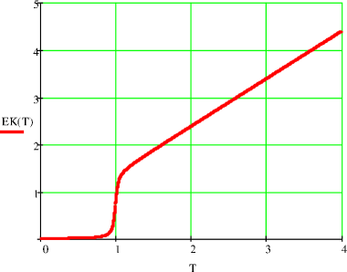
Figure 1: The average energy ${\bar{E}}$ $(=EK(T))$ of an acceleration surface per a hole as a function of the absolute temperature $T$, when the number of the holes on the surface is $N=100$. The absolute temperature $T$ has been expressed in the units of $T_{C}$, and the average energy ${\bar{E}}$ in the units of $k_{B}T_{C}$. If $T<T_{C}$, ${\bar{E}}$ is effectively zero, which means that the black holes on the acceleration surface are in vacuum. When $T=T_{C}$, the curve ${\bar{E}}={\bar{E}}(T)$ is practically vertical, which indicates a phase transition at the temperature $T=T_{C}$. During this phase transition the black holes on the acceleration surface are excited from the vacuum to the second excited states. The latent heat per a hole corresponding to this phase transition is ${\bar{L}}=2(\ln 2)k_{B}T_{C}\approx 1.4k_{B}T_{C}$. When $T>T_{C}$, the curve ${\bar{E}}={\bar{E}}(T)$ is approximately linear.

Our analysis shows that the characteristic, or Unruh temperature $T_{C}$ plays a crucial role in the statistics and the thermodynamics of spacetime. The Unruh temperature is the lowest possible temperature an acceleration surface may have, and at the Unruh temperature a phase transition occurs with a sudden increase in the energy of the acceleration surface.

It is interesting to consider the microphysical reason for the phase transition observed. What happens to the quantum states of the Planck size black holes constituting an acceleration surface during the phase transition? Combining Eqs.(4.4) and (4.10) we find that the average value of the quantum number $n$ characterizing the quantum states of an individual hole on an acceleration surface at the temperature $T=1/\beta$ is:

$${\bar{n}}=\frac{2\pi c}{(\ln 2)a\hbar}{\bar{E}}(\beta).$$ (108)

If we substitute for ${\bar{E}}(\beta)$ the quantity ${\bar{L}}$ of Eq.(4.26), which gives the average latent heat per a hole on the surface, we get:

$${\bar{n}}=2.$$ (109)

The physical meaning of this result is obvious: It means that during the phase transition the Planck size black holes on the acceleration surface become excited from the ground state to the second excited state. In this process the holes absorb quanta of energy from the matter fields until the holes are, in average, in the second excited state. The Unruh effect is a process inverse to the excitations of the holes, and it is caused by the de-excitations of the holes from the second excited state to the ground state.

IV.5 Zero Point Energy

Before closing the discussion about the energy of an acceleration surface it is appropriate to return to Eq.(4.2), which gives the precise expression to the total energy $E(\beta)$ of an acceleration surface as a function of its inverse temperature $\beta$. One finds that although the quantity ${\bar{E}}(\beta)$ vanishes for large $N$ and low temperature, the quantity $E(\beta)$ does not: In the low temperature limit $T\rightarrow 0$, where $\beta T_{C}\longrightarrow\infty$, the first term inside the brackets on the right hand side of Eq.(4.2) goes to unity. As a consequence we have:

$$\lim_{T\rightarrow 0}E(\beta)=k_{B}T_{C}\ln 2.$$ (110)

So we see that in our model the total energy of an acceleration surface has a certain non-vanishing zero point value.

V Entropy of an Acceleration Surface

V.1 Entropy vs Temperature

We shall now turn our attention to the entropy of an acceleration surface. How does the entropy of an acceleration surface depend on its temperature? How does it depend on the energy? Finally, we have the most interesting question of all: How does the entropy of an acceleration surface depend on its area? In particular, what is the relationship between the acceleration surface entropy and the Bekenstein-Hawking entropy of black holes?

In general, the entropy $S$ of any system obeys the relationship:

$$F=E-TS,$$ (111)

where

$$F:=-k_{B}T\ln Z$$ (112)

is the Helmholtz free energy of the system. So we find that the entropy of any system may be expressed as a function of its inverse temperature $\beta$, in natural units, as:

$$S(\beta)=\beta E(\beta)+\ln Z(\beta).$$ (113)

Using Eqs.(3.16) and (4.2) we get an expression to the entropy of an acceleration surface:

$$S(\beta)=\biggl{[}\frac{2^{\beta T_{C}}}{2^{\beta T_{C}}-2}-\frac{(N+1)2^{\beta T_{C}}}{(2^{\beta T_{C}}-1)^{(}N+2)-2^{\beta T_{C}}+1}\biggr{]}(\ln 2)\beta T_{C}+\ln\biggl{\{}\frac{1}{2^{\beta T_{C}}-2}\biggl{[}1-\biggl{(}\frac{1}{2^{\beta T_{C}}-1}\biggr{)}^{N+1}\biggr{]}\biggr{\}},$$ (114)

whenever $T\neq T_{C}$.

The first observation one may make about the properties of the entropy $S(\beta)$ is that in the limit, where $T\rightarrow 0$, which means that $\beta\rightarrow\infty$, we have:

$$\lim_{T\rightarrow 0}S(\beta)=0$$ (115)

for all $N$. In other words, our system obeys the third law of thermodynamics. Since $N$ is assumed to be of the order $10^{70}$, it is useful to consider the rescaled entropy

$${\bar{S}}(\beta):=\frac{S(\beta)}{N},$$ (116)

instead of the entropy $S(\beta)$ itself. One finds that, in general:

$${\bar{S}}(\beta)=\frac{1}{N}\frac{2^{\beta T_{C}}}{2^{\beta T_{C}}-2}(\ln 2)\beta T_{C}-\frac{N+1}{N}\frac{2^{\beta T_{C}}}{(2^{\beta T_{C}}-1)^{N+2}-2^{\beta T_{C}}+1}(\ln 2)\beta T_{C}+\frac{1}{N}\ln\biggl{\{}\frac{1}{2^{\beta T_{C}}-2}\biggl{[}1-\biggl{(}\frac{1}{2^{\beta T_{C}}-1}\biggr{)}^{N+1}\biggr{]}\biggr{\}}.$$ (117)

V.1.1 The case $T<T_{C}$

Consider first the special case, where $T<T_{C}$. In that case $2^{\beta T_{C}}-1>1$, and therefore $(2^{\beta T_{C}}-1)^{N}$ becomes huge for large $N$. So we observe that

$$\lim_{N\rightarrow\infty}{\bar{S}}(\beta)=0,$$ (118)

whenever $T<T_{C}$. In other words, the rescaled entropy effectively vanishes for large $N$, when $T<T_{C}$. The entropy $S(\beta)$ itself has the property:

$$\lim_{N\rightarrow\infty}S(\beta)=\frac{2^{\beta T_{C}}}{2^{\beta T_{C}}-1}(\ln 2)\beta T_{C}-\ln(2^{\beta T_{C}}-2)$$ (119)

which, in the natural units, is of the order of unity, when $T<T_{C}$. We shall see in a moment that $S(\beta)$ is of the order of $N$ in the natural units, when $T>T_{C}$. So we may conclude that not only the does rescaled entropy ${\bar{S}}(\beta)$, but also the entropy $S(\beta)$ itself effectively vanishes in the large $N$ limit, when $T<T_{C}$.

V.1.2 The case $T>T_{C}$

When $T>T_{C}$, $0<2^{\beta T_{C}}-1<1$, and $(2^{\beta T_{C}}-1)^{N}$ becomes very small for large $N$. Hence it follows that when $T>T_{C}$, we may write for large $N$:

$${\bar{S}}(\beta)=\frac{2^{\beta T_{C}}}{2^{\beta T_{C}}-1}(\ln 2)\beta T_{C}-\ln(2^{\beta T_{C}}-1).$$ (120)

When the temperature is very high, i.e. $T>>T_{C}$, then $\beta T_{C}$ is very small, and we find:

$${\bar{S}}(\beta)=\ln(\frac{T}{T_{C}})-\ln(\ln 2)+\mathcal{O}[(\beta T_{C})],$$ (121)

where $\mathcal{O}[(\beta T_{C})]$ denotes the terms, wich are of the order $(\beta T_{C})^{1}$, or higher. Hence we observe that in very high temperatures the entropy depends, in effect, logarithmically on the temperature $T$.

V.1.3 The case $T=T_{C}$

It only remains to consider the case, where $T=T_{C}$. Using Eqs.(3.17), (4.22) and (5.3) we find:

$${\bar{S}}(T_{C})=\ln 2+\frac{1}{N}\ln N.$$ (122)

Moreover, because

$${\bar{S}}^{\prime}(T)=\frac{1}{T}{\bar{E}}^{\prime}(T),$$ (123)

which follows from Eqs.(4.1) and (5.3), together with the result:

$$\frac{d\beta}{dT}=-\frac{1}{T^{2}},$$ (124)

we find, using Eq.(4.23):

$${\bar{S}}^{\prime}(T_{C})=\frac{(\ln 2)^{2}}{6T_{C}}N+\mathcal{O}(1),$$ (125)

where $\mathcal{O}(1)$ denotes the terms, which are of the order $N^{0}$, or less. So we see that when $T=T_{C}$, the first derivative ${\bar{S}}^{\prime}(T)$ of ${\bar{S}}(T)$ is, in effect, proportional to $N$. For large $N$ this indicates a rapid jump in the values of ${\bar{S}}(T)$ at the point, where $T=T_{C}$. The magnitude of this jump is, in natural units,

$$\Delta{\bar{S}}=2\ln 2,$$ (126)

which may be obtained from Eq.(5.10), if we substitute $1/T_{C}$ for $\beta$.

The conclusions made above are confirmed by numerical investigations. In Fig. 2 we have made a plot of the graph of the function ${\bar{S}}(T)$ in the special case, where $N=100$. As one may observe, ${\bar{S}}(T)$ is virtually zero, when $T<T_{C}$. At the point, where $T=T_{C}$, the curve ${\bar{S}}={\bar{S}}(T)$ is almost vertical, and there is a discrete jump $\Delta{\bar{S}}$, which is about $1.4\approx 2\ln 2$, in the values of ${\bar{S}}(T)$. When $T>>T_{C}$, ${\bar{S}}(T)$ depends logarithmically on $T$.

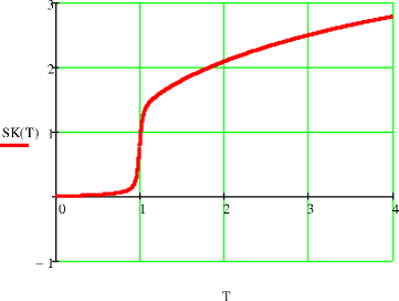
Figure 2: The rescaled entropy ${\bar{S}}$ $(=SK(T))$ (average entropy per a hole) of an acceleration surface as a function of the absolute temperature $T$ of spacetime, when the number of black holes on the surface is $N=100$. The absolute temperature has been expressed in the units of $T_{C}$, and the rescaled entropy ${\bar{S}}$ in the units of $k_{B}$. If $T<T_{C}$, ${\bar{S}}$ is effectively zero. At the temperature $T=T_{C}$ corresponding to the phase transition, the curve ${\bar{S}}={\bar{S}}(T)$ is practically vertical, and there is a discrete jump $\Delta{\bar{S}}=2(\ln 2)k_{B}\approx 1.4k_{B}$ in the values of ${\bar{S}}$. Finally, when $T>T_{C}$, there is an approximately logarithmic dependence of ${\bar{S}}$ on $T$.

V.2 Entropy vs Area

We shall now turn our attention to the relationship between the area and the entropy of an acceleration surface. Our starting point is Eq.(5.13), which implies:

$$\frac{d{\bar{S}}}{d{\bar{E}}}=\frac{1}{T}.$$ (127)

Consider first the special case, where $T$ is very close to the characteristic temperature $T_{C}$. In that case we may write:

$$T=T_{C}+\Delta T,$$ (128)

where $\Delta T$, the difference between $T$ and $T_{C}$, may be approximated by an expression:

$$\Delta T=\frac{dT}{d{\bar{E}}}|_{E=E_{C}}\,\Delta{\bar{E}},$$ (129)

where

$$\Delta{\bar{E}}:={\bar{E}}-{\bar{E}}_{C},$$ (130)

and ${\bar{E}}_{C}$ is given by the right hand side of Eq.(4.22), i. e. ${\bar{E}}_{C}$ is the average energy per a hole corresponding to the temperature $T_{C}$. Because $\frac{dT}{d{\bar{E}}}=1/\frac{d{\bar{E}}}{dT}$ we find, using Eq.(4.23):

$$\Delta T=\frac{6}{N(\ln 2)^{2}}\,({\bar{E}}-{\bar{E}}_{C})+\mathcal{O}(N^{-2}),$$ (131)

where $\mathcal{O}(N^{-2})$ denotes the terms, which are of the order $N^{-2}$, or less. Since $N$ is assumed to be very large, we may observe that close to the characteristic temperature $T_{C}$ the right hand side of Eq.(5.17) is effectively independent of ${\bar{E}}$. This is the same conclusion which we may arrive at, if we look at the curve ${\bar{E}}={\bar{E}}(T)$ of Fig. 1: When $E$ lies within the interval $[0,2T_{C}\ln 2]$, $T$ is close to $T_{C}$, and the curve ${\bar{E}}={\bar{E}}(T)$ is practically vertical. This means that the temperature $T$ is, in effect, a constant function of ${\bar{E}}$, when $0<{\bar{E}}<2T_{C}\ln 2$. So we find that when $0<{\bar{E}}<2T_{C}\ln 2$, we may write Eq.(5.17), as an excellent approximation, as:

$$\frac{d{\bar{S}}}{d{\bar{E}}}=\frac{1}{T_{C}}.$$ (132)

Because the characteristic temperature $T_{C}$ may identified as the Unruh temperature $T_{U}$ of Eq.(2.23), and the rescaled entropy ${\bar{S}}$ goes to zero together with the average energy ${\bar{E}}$, Eq.(5.22) implies, in the natural units,

$${\bar{S}}({\bar{E}})=\frac{2\pi}{a}{\bar{E}}$$ (133)

or, in the SI units,

$${\bar{S}}({\bar{E}})=\frac{2\pi k_{B}c}{\hbar a}{\bar{E}},$$ (134)

whenever $0<{\bar{E}}<2T_{C}\ln 2$. Multiplying the both sides of Eq.(5.25) by $N$ we get the relationship between the entropy $S$ and the energy $E$ of an acceleration surface, when $0<E<2NT_{C}\ln 2$:

$$S(E)=\frac{2\pi k_{B}c}{\hbar a}E.$$ (135)

If we use Eq.(2.26), which gives the relationship between the area $A$ and the energy $E$ of an acceleration surface, we may convert Eq.(5.25) to a relationship between the entropy and the area of an acceleration surface. In the natural units we get:

$$S(A)=\frac{1}{2}A$$ (136)

which, in the SI units, takes the form:

$$S(A)=\frac{1}{2}\frac{k_{B}c^{3}}{\hbar G}A.$$ (137)

Eq.(5.27) is most remarkable. It gives an expression for the entropy of an acceleration surface when the surface is, from the point of view of an observer at rest with respect to the acceleration surface, in thermal equilibrium with the matter fields, and the temperature is close to the Unruh temperature $T_{U}$ measured by the observer. Eq.(5.27) states that in this case the entropy of an acceleration surface is, in natural units, exactly one-half of the area of the surface. Hence we have obtained a result which is closely related, although not quite identical, to the Bekenstein-Hawking entropy law. According to the Bekenstein-Hawking entropy law the entropy of a black hole event horizon is, in natural units, one-quarter of its area. kymmenen ; yksitoista So we have obtained for the acceleration surface entropy an expression, which is exactly twice the entropy of a black hole event horizon with the same area.

The reason for the difference by the factor of two between the right hand side of Eq.(5.27) and that of the Bekenstein-Hawking entropy law has been considered in details in Ref. kolme . At least for a Schwarzschild black hole the reason for the difference is easy to understand, if we consider Eq.(2.27), which gives the ADM mass $M_{ADM}$ of the hole in terms of the surface gravity $\kappa$ and the area $A$ of its event horizon. Differentiating the both sides of Eq.(2.27) we get:

$$dM_{ADM}=\frac{1}{4\pi}A\,d\kappa+\frac{1}{4\pi}\kappa\,dA=\frac{1}{8\pi}\kappa\,dA,$$ (138)

where we have used the result: kuusitoista

$$A\,d\kappa=-\frac{1}{2}\kappa\,dA.$$ (139)

If we identify $dM_{ADM}$ as the change in the thermal energy of the hole, the fundamental thermodynamical relation $\delta Q=T\,dS$ implies that $dS=\frac{1}{4}\,dA$, provided that the temperature $T=\frac{\kappa}{2\pi}$. In contrast, differentiation of the both sides of Eq.(2.25), which gives the thermal energy $Q_{as}$ of an acceleration surface, yields the result:

$$\delta Q_{as}=\frac{1}{4\pi}a\,dA,$$ (140)

which follows from the fact that the proper acceleration $a$ has been kept as a constant during the differentiation. Hence the relation $\delta Q=T\,dS$ implies that $dS=\frac{1}{2}\,dA$, when $T=T_{U}=\frac{a}{2\pi}$. So we see that the basic difference between the thermodynamical properties of black hole event horizons and those of acceleration surfaces is that for black hole event horizons a change in the area implies a certain change in its surface gravity, whereas for acceleration surfaces the change in the area preserves the proper acceleration $a$, which plays the role of surface gravity for acceleration surfaces, as a constant. It is this difference, which is the reason for the different entropies of black hole event horizons and acceleration surfaces.

One of the crucial points in the derivation of the expression given by Eq.(5.27) for the entropy $S(A)$ of an acceleration surface, when $T$ is close to $T_{C}$, was an observation that close to $T_{C}$ the temperature $T$ is virtually independent of the energy $E$ of the acceleration surface. However, as we saw in our discussion, an independence of the temperature $T$ on the energy $E$ is a valid approximation if and only if ${\bar{E}}$ is smaller than $2T_{C}\ln 2$, which means that $E$ is smaller than the critical energy

$$E_{crit}:=2NT_{C}\ln 2=\frac{Na\ln 2}{\pi}$$ (141)

or, in SI units:

$$E_{crit}=\frac{N\hbar a\ln 2}{\pi c}.$$ (142)

If we substitute $E_{crit}$ for $Q_{as}$ in Eq.(2.26), and solve the area $A$ of an acceleration surface, we find that the critical energy $E_{crit}$ corresponds to the critical area

$$A_{crit}:=\frac{4\pi}{a}E_{crit}=4N\ln 2$$ (143)

or, in SI units:

$$A_{crit}=4N\ell_{Pl}^{2}\ln 2,$$ (144)

where $\ell_{Pl}$ is the Planck length. The entropy of an acceleration surface is given, as an excellent approximation, by Eq.(5.27), whenever its area $A$ is less than the critical area $A_{crit}$. When $A=A_{crit}$, the microscopic black holes are, in average, on the second excited state.

What happens, when $A>A_{crit}$? When $A>A_{crit}$, the black holes on the acceleration surface are excited, in average, above the second excited state, and the temperature exceeds the Unruh temperature $T_{U}=T_{C}$. In that case Eq.(5.27) is no more valid, and we must find another expression for the entropy of an acceleration surface in terms of its area $A$.

Our starting point is Eq.(5.10), which gives the rescaled entropy ${\bar{S}}(\beta)$ of an acceleration surface in terms of its inverse temperature $\beta$, when $T>T_{C}$ and $N$ is very large. As the first step we solve the quantity $2^{\beta T_{C}}$ in terms of ${\bar{E}}$ from Eq.(4.15), which is valid, when $T>T_{C}$, and substitute the resulting expression in Eq.(5.10). We get:

$${\bar{S}}({\bar{E}})=\frac{{\bar{E}}}{T_{C}\ln 2}\ln\biggl{(}\frac{\bar{E}}{{\bar{E}}-T_{C}\ln 2}\biggr{)}+\ln\biggl{(}\frac{{\bar{E}}}{T_{C}\ln 2}-1\biggr{)}.$$ (145)

As one may observe, Eq.(5.35) reduces to Eq.(5.23), when ${\bar{E}}=2T_{C}\ln 2$. So we find that the entropy of an acceleration surface may be written in terms of its total energy as:

$$S(E)=\frac{E}{T_{C}\ln 2}\ln\biggl{(}\frac{E}{E-NT_{C}\ln 2}\biggr{)}+N\ln\biggl{(}\frac{E-NT_{C}\ln 2}{NT_{C}\ln 2}\biggr{)}$$ (146)

which, in turn, may be converted to a relationship between entropy and area:

$$S(A)=\frac{1}{2\ln 2}A\ln\biggl{(}\frac{2A}{2A-A_{crit}}\biggr{)}+N\ln\biggl{(}\frac{2A-A_{crit}}{A_{crit}}\bigg{)}$$ (147)

or, in SI units:

$$S(A)=\frac{1}{2\ln 2}\frac{k_{B}c^{3}}{\hbar G}A\ln\biggl{(}\frac{2A}{2A-A_{crit}}\biggr{)}+Nk_{B}\ln\biggl{(}\frac{2A-A_{crit}}{A_{crit}}\biggr{)},$$ (148)

which is valid, whenever $A>A_{crit}$. As one may observe, the entropy is no more a linear function of the area, but it involves certain logarithmic functions of the area.

When the area $A$ is close to the critical area $A_{crit}$, the first term on the right hand side of Eq.(5.38) will dominate. However, when $A>>A_{crit}$, which means that the temperature of the acceleration surface is very much higher than its Unruh temperature $T_{U}$ and the black holes on the surface lie on highly excited states, the second term will dominate. In this limit we may write, in effect:

$$S(A)=Nk_{B}\ln(\frac{A}{A_{crit}}),$$ (149)

where we have neglected the physically irrelevant additive constants from our expression of entropy. In other words, in the high temperature limit the entropy of an acceleration surface will no more depend linearly but logarithmically on its area. This result reproduces the findings of Ref. kolme .

To conclude, we have found that when $A<A_{crit}$, the entropy of an acceleration surface is, in natural units, exactly one-half of its area. However, when $A>A_{crit}$, the linear dependence between entropy and area breaks down, and when $A>>A_{crit}$, the entropy depends logarithmically on the area. These conclusions of ours are confirmed by numerical investigations. In Fig. 3 we have made a plot of $S$ as a function of $A$, when $N=100$, and both $S$ and $A$ have been expressed in the units of $A_{crit}$. One finds that when $A<A_{crit}$, $S=\frac{1}{2}A$ as an excellent approximation. However, when $A>A_{crit}$, $S$ will no more depend linearly on $A$.

Figure 3: The entropy $S$ $(=SA(T))$ of an acceleration surface as a function of the area $A$ of the surface, when $N=100$. Both $S$ and $A$ have been expressed in the units of the critical area $A_{crit}$. When $A<A_{crit}$, $S=\frac{1}{2}A$ as an excellent approximation. However, when $A>A_{crit}$, $S$ will no more depend linearly on $A$.

V.3 Equation of State

If one knows the entropy $S$ and the temperature $T$ of any system, one may calculate its pressure $p$:

$$p=\biggl{(}\frac{\partial S}{\partial V}\biggr{)}_{N,E}T.$$ (150)

The entropy of a perfect classical gas, for instance, is proportional to the number $N$ of its molecules, and it depends logarithmically on its volume $V$. Therefore Eq.(5.40) implies for a perfect classical gas the well known equation of state:

$$pV=Nk_{B}T.$$ (151)

What is the corresponding equation of state of an acceleration surface? For two-dimensional systems, such as acceleration surfaces, the pressure $p$ is replaced by the surface tension

$$\sigma:=\biggl{(}\frac{\partial S}{\partial A}\biggr{)}_{N,E}T.$$ (152)

The physical meaning of the surface tension $\sigma$ is that if the area $A$ of the surface is increased by $dA$, the work done on the surface during the process is

$$dW=\sigma\,dA.$$ (153)

Because the work done on an acceleration surface is ultimately converted to heat we find, using Eq.(2.26), that the surface tension of an acceleration surface with a proper acceleration $a$ is, in general:

$$\sigma_{as}=\frac{c^{2}a}{4\pi G}.$$ (154)

So we see that the surface tension of an acceleration surface depends on its proper acceleration $a$ only, and it is independent of the area $A$ and the temperature $T$ of the surface. The equation of state of an acceleration surface gives a relationship between the surface tension $\sigma_{as}$ (and therefore the proper acceleration $a$), the area and the temperature of the surface. If $A<A_{crit}$, we may use Eq.(5.27), and the resulting equation of state is:

$$\sigma_{as}=\frac{1}{2}T$$ (155)

or, in SI units:

$$\sigma_{as}=\frac{1}{2}\frac{k_{B}c^{3}}{\hbar G}T.$$ (156)

If $A<A_{crit}$, then $T=T_{C}=T_{U}$. If we substitute $T_{C}$ for $T$ in Eq.(5.47), we recover Eq.(5.45).

If $A>A_{crit}$, we must use Eq.(5.37). In that case Eq.(5.42) implies the following equation of state:

$$\sigma_{as}=\frac{1}{2\ln 2}\frac{k_{B}c^{3}}{\hbar G}\biggl{[}\ln\biggl{(}\frac{2A}{2A-A_{crit}}\biggr{)}-\frac{A_{crit}}{2A-A_{crit}}\biggr{]}T+\frac{2Nk_{B}}{2A-A_{crit}}T.$$ (157)

In the very high temperatures, where $A>>A_{crit}$, we may write Eq.(5.47), in effect, as:

$$\sigma_{as}A=Nk_{B}T,$$ (158)

which is analogous to Eq.(5.41).

VI Concluding Remarks

In this paper we have considered the partition function of spacetime in gravitational physics. The calculation of the partition function was based on a model of spacetime, where spacetime was assumed to be a specific graph, with Planck size quantum black holes on its vertices, and where the macroscopic properties of spacetime were reduced to the horizon area eigenstates of the holes. In the macroscopic level, the thermodynamical system under consideration was taken to be the so called acceleration surface of spacetime. In broad terms, acceleration surface may be described as a spacelike two-surface of spacetime, whose every point is accelerated uniformly, with the same proper acceleration, to the direction of a spacelike unit normal vector field of the surface. For acceleration surfaces it is possible to define a quantity which describes the thermal energy of the surface. In the classical level, Einstein’s field equation with a vanishing cosmological constant may be shown to be a simple and straightforward consequence of a thermodynamical equation, which describes the exchange of energy between an acceleration surface and the matter which flows through the surface, and which we called as the ”fundamental equation” of the thermodynamics of spacetime. In the quantum level, the Planck size quantum black holes lying on the acceleration surface were assumed to obey certain independence- and statistical postulates. Using these postulates, together with our definition of the concept of thermal energy of an acceleration surface, we were able to write the partition function of the surface. We were able to find an explicit and surprisingly simple expression for the partition function of an acceleration surface in terms of the inverse temperature $\beta$ of the surface, and to work out the physical consequences of the partition function.

We found that acceleration surface possesses, from the point of view of an observer at rest with respect to the surface, a certain characteristic temperature $T_{C}$, which may be identified as the Unruh temperature $T_{U}$ measured by the observer. When the temperature of an acceleration surface is, from the point of view of our observer, less than its Unruh temperature, the energy of the acceleration surface is effectively zero. However, when the temperature $T$ of the surface is the same as its Unruh temperature, the surface performs a phase transition, where the Planck size quantum black holes on the surface are, in average, excited from the vacuum to the second excited states. During this phase transition the temperature of the surface remains the same, but its energy jumps from zero to a certain finite, well-defined value. The latent heat corresponding to the phase transition equals to the energy which the surface has, from the point of view of our observer, when all of the Planck size quantum black holes on the surface lie on the second excited state. When the temperature exceeds the Unruh temperature $T_{U}$, the energy of the surface depends, in effect, linearly on the temperature $T$.

The same investigations were performed for the entropy of an acceleration surface. As in the case of energy, it was found that the Unruh temperature $T_{U}$ of the surface plays an important role. When $T<T_{U}$, the entropy of an acceleration surface is effectively zero, but when $T=T_{U}$, there is a rapid increase in its entropy, which corresponds to the phase transition performed by the surface. When $T>T_{U}$, there is an effective logarithmic dependence of the entropy of an acceleration surface on its temperature.

The entropy $S$ of an acceleration surface may be expressed as a function of the area $A$ of the surface. We found that there is a certain critical area $A_{crit}$, which is the area an acceleration surface has, when all of the Planck size black holes lying on the surface are in the second excited state. When $A<A_{crit}$, the entropy of the surface is, in natural units, almost exactly one-half of the area $A$. However, when $A>A_{crit}$, there is no more a linear dependence between the area and the entropy of the surface, but certain correction terms involving logarithms of the area will appear. When $A>>A_{crit}$, which means that the temperature of the acceleration surface vastly exceeds its Unruh temperature and the black holes are in highly excited states, there is, in effect, a logarithmic dependence of the entopy of the surface on its area.

The most important physical result of this paper is the existence of a phase transition, when the temperature $T$ of an acceleration surface equals to its characteristic temperature $T_{C}$. Since the Planck size quantum black holes constituting an acceleration surface are in vacuum, when $T<T_{C}$, and suddenly jump, in average, to the second excited state, when $T=T_{C}$, we may view the characteristic temperature $T_{C}$ as the lowest possible temperature, which an acceleration surface may have from the point of view of an observer moving along with the surface. When acceleration surface is in thermal equilibrium with the radiation fields, it both emits and absorbs radiation with the temperature $T_{C}$. As a result, an accelerated observer will detect thermal radiation with a characteristic temperature $T_{C}$, which is proportional to the proper acceleration $a$, even when the radiation fields are, from the point of view all inertial observers, in vacuum. In other words, our model predicts the Unruh effect, and provides that effect with an explanation, which may be traced back to the microscopic properties of spacetime: In the same way as the thermal radiation of ordinary matter is caused by the de-excitations of its atoms and molecules, the thermal radiation observed by an accelerated observer is, according to our model, caused by the de-excitations of the Planck size quantum black holes constituting spacetime. The characteristic temperature $T_{C}$ may be identified as the Unruh temperature $T_{U}$ measured by an accelerated observer, and this identification fixed the only undetermined parameter of our model. We found in our paper that our model predicts not only the Unruh effect, but also the Hawking effect. That conclusion was drawn from an observation that every horizon of spacetime, black hole event horizons included, may be considered as a limit of an appropriate acceleration surface, when the proper acceleration $a$ of that surface goes to infinity.

To conclude, there were three key elements in our approach to the partition function of spacetime. The first of them was our decision to focus our attention to the acceleration surfaces, and to take acceleration surfaces as the physical systems under study in gravitational physics. The second element was a definition of the concept of energy of an acceleration surface in a certain manner. As we saw in Section 2, that definition implies Einstein’s field equation with a vanishing cosmological constant in classical spacetime. Finally, the third element was to construct a microscopic model of spacetime out of Planck size quantum black holes, which were assumed to obey certain very simple quantum mechanical and statistical postulates. An approach based on these key elements allowed us to find an explicit and surprisingly simple expression for the partition function of spacetime, and that partition function implied, among other things, the Unruh and the Hawking effects. In this sense our model, in its all simplicity, may hold some promises for the future. It remains to be seen, whether the ideas employed in this paper in the calculation of the partition function may be utilized in the calculation of the corresponding quantum mechanical objects, such as the wave function and the propagator, of spacetime.

Appendix A Calculation of the Partition Function

In this Appendix derive the expression (3.16) for the partition function $Z(\beta)$ of an acceleration surface with a proper acceleration $a$. Defining a quantity

$$q:=2^{-\beta T_{C}}$$ (159)

one may write the sums $Z_{1}(\beta)$ and $Z_{2}(\beta)$ of Eqs.(3.15a) and (3.15b) as:

$$Z_{1}(\beta) = \frac{1}{2}\sum_{n=1}^{N}(2q)^{n},$$ (160a)

$$Z_{2}(\beta) = \sum_{n=N+1}^{\infty}\biggl{[}\sum_{k=0}^{N}\left(\begin{array}[]{ccc}n-1\\ k\end{array}\right)q^{n}\biggr{]}.$$ (160d)

Since $\beta$ and $T_{C}$ are both positive, $q<1$. $Z_{1}(\beta)$ is just a geometrical series, and we get:

$$Z_{1}(\beta)=q\frac{1-(2q)^{N}}{1-2q},$$ (161)

provided that $q\neq\frac{1}{2}$. If $q=\frac{1}{2}$, we have

$$Z_{1}(\beta)=\frac{1}{2}N.$$ (162)

$Z_{2}(\beta)$ is much more difficult to calculate than $Z_{1}(\beta)$. When calculating $Z_{2}(\beta)$, one of the key ideas is to write the right hand side of Eq.(A2b) by means of the higher order derivatives of an appropriate function of $q$. Because, in general, an arbitrary binomial coefficient may be written as:

$$\left(\begin{array}[]{ccc}n\\ k\end{array}\right)=\frac{1}{k!}n(n-1)(n-2)...(n-k+1),$$ (163)

whenever $k>0$, and $\left(\begin{array}[]{ccc}n\\ k\end{array}\right)=1$, when $k=0$, one obtains a general formula

$$\left(\begin{array}[]{ccc}n\\ k\end{array}\right)q^{m}=\frac{1}{k!}q^{m-n+k}\frac{d^{k}}{dq^{k}}q^{n},$$ (164)

which yields:

$$\left(\begin{array}[]{ccc}n-1\\ k\end{array}\right)q^{n}=\frac{1}{k!}q^{k+1}\frac{d^{k}}{dq^{k}}q^{n-1}.$$ (165)

So we find:

$$Z_{2}(\beta)=\sum_{n=N+1}^{\infty}\biggl{[}\sum_{k=0}^{N}\frac{1}{k!}q^{k+1}\frac{d^{k}}{dq^{k}}q^{n-1}\biggr{]}.$$ (166)

Since one of the sums has a finite number of terms, we may change the order of the summation, and we get:

$$Z_{2}(\beta)=\sum_{k=0}^{N}\biggl{[}\frac{1}{k!}q^{k+1}\frac{d^{k}}{dq^{k}}(q^{N}\sum_{n=0}^{\infty}q^{n})\biggr{]}.$$ (167)

Because $|q|<1$, the geometric sum on the right hand side of Eq.(A9) will converge, and we have:

$$Z_{2}(\beta)=\sum_{k=0}^{N}\biggl{[}\frac{1}{k!}q^{k+1}\frac{d^{k}}{dq^{k}}(\frac{q^{N}}{1-q})\biggr{]}.$$ (168)

As one may observe, we have managed to reduce a double sum with an infinite number of terms into a simple sum with a finite number of terms.

As the next step we employ the following formula, which is a consequence of the product rule of differentiation:

$$\frac{d^{k}}{dq^{k}}[f_{1}(q)f_{2}(q)]=\sum_{m=0}^{k}\left(\begin{array}[]{ccc}k\\ m\end{array}\right)f_{1}^{(k-m)}(q)f_{2}^{(m)}(q)$$ (169)

for arbitrary smooth functions $f_{1}(q)$ and $f_{2}(q)$. If we define:

$$f_{1}(q) := q^{N},$$ (170a)

$$f_{2}(q) := \frac{1}{1-q},$$ (170b)

we have:

$$f_{1}^{(k-m)}(q) = \frac{N!}{(N-k+m)!}q^{N-k+m},$$ (171a)

$$f_{2}^{(m)}(q) = m!(1-q)^{-m-1},$$ (171b)

and therefore Eq.(A10) takes the form:

$$Z_{2}(\beta)=\frac{q^{N+1}}{1-q}\sum_{k=0}^{N}\biggl{[}\sum_{m=0}^{k}\frac{N!}{(k-m)!(N-k+m)!}(\frac{q}{1-q})^{m}\biggr{]}.$$ (172)

When obtaining Eq.(A14) we have used the formula:

$$\left(\begin{array}[]{ccc}k\\ m\end{array}\right)=\frac{k!}{m!(k-m)!}.$$ (173)

Using Eq.(A15) we find:

$$Z_{2}(\beta)=\frac{x^{N+1}}{(1+x)^{N}}\sum_{k=0}^{N}\biggl{[}\sum_{m=0}^{k}\left(\begin{array}[]{ccc}N\\ k-m\end{array}\right)x^{m}\biggr{]},$$ (174)

where we have defined a new variable

$$x:=\frac{q}{1-q}.$$ (175)

Because $0<q<1$, $x$ is positive.

Now, it is possible to rearrange the sums on the right hand side of Eq.(A16). As a result we get:

$$Z_{2}(\beta)=\frac{x^{N+1}}{(1+x)^{N}}\sum_{n=0}^{N}\biggl{[}\left(\begin{array}[]{ccc}N\\ n\end{array}\right)\sum_{k=0}^{N-n}x^{k}\biggr{]}.$$ (176)

Because

$$\sum_{k=0}^{N-n}x^{k}=\frac{1-x^{N-n+1}}{1-x},$$ (177)

when $x\neq 1$, and

$$\sum_{k=0}^{N-n}x^{k}=N-n+1,$$ (178)

when $x=1$, we have:

$$Z_{2}(\beta)=\frac{x^{N+1}}{(1+x)^{N}}\frac{1}{1-x}\biggl{[}\sum_{n=0}^{N}\left(\begin{array}[]{ccc}N\\ n\end{array}\right)-x^{N+1}\sum_{n=0}^{N}\left(\begin{array}[]{ccc}N\\ n\end{array}\right)x^{-n}\biggr{]},$$ (179)

when $x\neq 1$, and

$$Z_{2}(\beta)=\frac{1}{2^{N}}\sum_{m=0}^{N}\biggl{[}\left(\begin{array}[]{ccc}N\\ n\end{array}\right)(N-n+1)\biggr{]},$$ (180)

when $x=1$. Using the formulas:

$$\sum_{n=0}^{N}\left(\begin{array}[]{ccc}N\\ n\end{array}\right) = 2^{N},$$ (181c)

$$\sum_{n=0}^{N}n\left(\begin{array}[]{ccc}N\\ n\end{array}\right) = N2^{N-1},$$ (181f)

$$\sum_{n=0}^{N}\left(\begin{array}[]{ccc}N\\ n\end{array}\right)(\frac{1}{x})^{n} = \biggl{(}1+\frac{1}{x}\biggr{)}^{N},$$ (181i)

we get:

$$Z_{2}(\beta)=\frac{x}{1-x}\biggl{[}(\frac{2x}{1+x})^{N}-x^{N+1}\biggr{]},$$ (182)

when $x\neq 1$, and

$$Z_{2}(\beta)=\frac{1}{2}N+1,$$ (183)

when $x=1$. When written in terms of the variable $q$, Eq.(A24) takes the form:

$$Z_{2}(\beta)=\frac{q^{N+1}}{1-2q}\biggl{[}2^{N}-\frac{q}{(1-q)^{N+1}}\biggr{]}.$$ (184)

Combining Eqs.(A2-A4), and (A26) we get, when $\beta\neq\frac{1}{T_{C}}$:

$$Z(\beta)=\frac{q}{1-2q}\biggl{[}1-\biggl{(}\frac{q}{1-q}\biggr{)}^{N+1}\biggr{]},$$ (185)

and

$$Z(\beta)=N+1,$$ (186)

when $\beta=\frac{1}{T_{C}}$. Using Eq.(A1) we find the final expression for the partition function, when $\beta\neq\frac{1}{T_{C}}$:

$$Z(\beta)=\frac{1}{2^{\beta T_{C}}-2}\biggl{[}1-\biggl{(}\frac{1}{2^{\beta T_{C}}-1}\biggr{)}^{N+1}\biggr{]},$$ (187)

which is Eq.(3.16).

Appendix B Properties of the Partition Function Near the Characteristic Temperature

In this Appendix we consider the energy of an acceleration surface, when the absolute temperature $T$ measured by an observer moving along with the surface is very close to the characteristic temperature $T_{C}$.

Our starting point is Eq.(3.16), which gives the precise epression for the partition function $Z(\beta)$ of an acceleration surface. Because $2^{\beta T_{C}}=2$, when $T=T_{C}$, we denote:

$$y:=2^{\beta T_{C}}-2,$$ (188)

and Eq.(3.16) takes the form:

$$Z(y)=\frac{1}{y}[1-(1+y)^{-N-1}].$$ (189)

When $T$ is close to $T_{C}$, $y$ is close to zero. When $y$ is close to zero we may write, using Newton’s binomial theorem:

$$(1+y)^{-N-1}=1-(N+1)y+\frac{(N+1)(N+2)}{2!}y^{2}-\frac{(N+1)(N+2)(N+3)}{3!}y^{3}+...,$$ (190)

and we get the Taylor expansion of $Z(y)$ around the point, where $y=0$:

$$Z(y)=(N+1)-\frac{(N+1)(N+2)}{2!}y+\frac{(N+1)(N+2)(N+3)}{3!}y^{2}-....$$ (191)

Applying the chain rule and the result

$$\frac{dy}{d\beta}=T_{C}(\ln 2)2^{\beta T_{C}}$$ (192)

we find:

$$E(\beta)=-\frac{\partial}{\partial\beta}\ln Z(\beta)=-\frac{Z^{\prime}(y)}{Z(y)}T_{C}(\ln 2)(y+2),$$ (193)

where $Z(y)$ is given by Eq.(B4) and

$$Z^{\prime}(y)=-\frac{(N+1)(N+2)}{2}+\frac{(N+1)(N+2)(N+3)}{3}y-\frac{(N+1)(N+2)(N+3)(N+4)}{8}y^{2}+...$$ (194)

One readily finds that

$$Z(0) = N+1,$$ (195a)

$$Z^{\prime}(0) = -\frac{(N+1)(N+2)}{2},$$ (195b)

which implies:

$$E(\frac{1}{T_{C}})=(N+2)T_{C}\ln 2.$$ (196)

Therefore, for very large $N$:

$${\bar{E}}(\frac{1}{T_{C}})=T_{C}\ln 2,$$ (197)

which is Eq.(4.22).

It is interesting to consider the derivative of ${\bar{E}}$ with respect to $T$, when $T=T_{C}$. Using Eq.(B6) we get:

$$\frac{dE}{dy}=\bigg{\{}\biggl{[}-\frac{Z^{\prime\prime}(y)}{Z(y)}+\biggl{(}\frac{Z^{\prime}(y)}{Z(y)}\biggr{)}^{2}\biggr{]}(y+2)-\frac{Z^{\prime}(y)}{Z(y)}\bigg{\}}T_{C}\ln 2,$$ (198)

and Eq.(B4) implies:

$$\frac{dE}{dT}|_{T=T_{C}}=\frac{(\ln 2)^{2}}{6}(N+2)(N+3),$$ (199)

where we have used the result:

$$\frac{dy}{dT}=-\frac{(\ln 2)T_{C}}{T^{2}}2^{\beta T_{C}}.$$ (200)

Hence we find that for very large $N$ we may write, in effect:

$$\frac{d{\bar{E}}}{dT}|_{T=T_{C}}=\frac{(\ln 2)^{2}}{6}N+\mathcal{O}(1),$$ (201)

which is Eq.(4.23). $\mathcal{O}(1)$ denotes the terms, which are of the order $N^{0}$, or less.

References

- (1) For emergent gravity see, for instance, T. Padmanabhan, arXiv: 0706.1654 and arXiv: 0802.1798, C. Barrelo, M. Wisser and S. Liberati, Int. J. Mod. Phys. D10 (2001) 799, T. Konopka, F. Markopoulou and S. Severini, Phys. Rev. D77 (2008) 104029, D. Oriti, arXiv: 0710.3276, S. Hossenfelder, Phys. Rev. D73 (2006) 105013, S. Hossenfelder, M. Bleicher, S. Hoffmann, J. Ruppert, S. Scherer and H. Stöcker, Phys. Lett. B575 (2003) 85.
- (2) J. Mäkelä, arXiv: 08053952.
- (3) J. Mäkelä, arXiv: 0805.3955.
- (4) J. Mäkelä and A. Peltola, Phys. Rev. D69 (2004) 124008.
- (5) J. Bekenstein, Lett. Nuovo Cim. 11 (1974) 467.
- (6) For papers on Bekenstein’s proposal see, for instance, J. D. Bekenstein and V. F. Mukhanov, Phys. Lett. B360 (1995) 7, P. C. Mazur, Phys. Rev. Lett. 57 (1987) 929, Y. Peleg, Phys. Lett. B356 (1995) 462, A. Barvinsky and G. Kunstatter, Phys. Lett. B389 (1996) 231, H. A. Kastrup, Phys. Lett. B389 (1996) 75, S. Hod, Phys. Rev. Lett. 81 (1998), S. Hod, Gen. Rel. Grav. 31 (1999) 1639, H. A. Kastrup, Class. Quant. Grav. 17 (2000) 3009, A. Barvinsky, S. Das and G. Kunstatter, Class. Quant. Grav. 18 (2001) 4845, J. D. Bekenstein, Int. J. Mod. Phys. A17S1 (2002) 21, J. D. Bekenstein and G. Gour, Phys. Rev. D66 (2002) 024005, J. Louko and J. Mäkelä, Phys. Rev. 54 4982, J. Mäkelä and P. Repo, Phys. Rev. D57 (1998) 4899, J. Mäkelä, P. Repo, M. Luomajoki and J. Piilonen, Phys. Rev. D64 (2001) 415, J. Mäkelä, Found. Phys. 32 (2002) 1809, J. Mäkelä, Phys. Lett. B390 (1997) 115, S. Hod, Class. Quant. Grav. 24 (2007) 4235.
- (7) C. W. Misner, K. S. Thorne and J. A. Wheeler, Gravitation (W. H. Freeman and Company, New York, 1973).
- (8) T. Jacobson, Phys. Rev. Lett. 75 (1995) 1260. See also, C. Eling, R. Guedens and T. Jacobson, Phys. Rev. Lett. 96 (2006) 121301, T. Jacobson, Found. Phys. 33 (2003) 323 and T. Jacobson in General Relativity and Relativistic Astrophysics: Eighth Canadian Conference (AIP Conference Proceedings 493, edited by C. P. Burgess and R. C. Myers (AIP, 1999)).
- (9) W. G. Unruh, Phys. Rev. D14 (1976) 870.
- (10) J. D. Bekenstein, Phys. Rev. D7 (1973) 2333.
- (11) S. W. Hawking, Commun. Math. Phys. 43 (1975) 199.
- (12) J. Mäkelä, gr-qc/0506087.
- (13) J. Mäkelä, gr-qc/0605098.
- (14) J. Mäkelä and A. Peltola, gr-qc/0612078 (accepted for publication in Int. J. Mod. Phys. D).
- (15) See, for example, T. Padmanabhan, Phys. Rept. 406 (2005) 49, Int. J. Mod. Phys. D13 (2004) 2293, Braz. J. Phys. 35 (2005) 362, A. Mukhopadhay and T. Padmanabhan, Phys. Rev. D74 (2006) 124023.
- (16) See, for example, R. M. Wald, General Relativity (University of Chicago Press, Chicago, 1984).
- (17) The role of the cosmological constant in the present observations of dark energy has been discussed, for example, by R. Bean, S. Carroll and M. Trodden, astro-ph/0510059.
- (18) D. Bernoulli, Hydrodynamica (1738) Section 10. (An English translation of this work may be found in The World of Mathematics, ed. by J. R. Newman (Tempus Books of Microsoft Press, Redmont, 1988)).
- (19) See, for instance, F. Mandl, Statistical Physics (John Wiley and Sons Ltd., Bristol, 1983).