On the Study of Richard Tom Robert Identity
Yeong-Shyeong Tsai
Department of Applied Mathematics, National Chung Hsing University, Taichung, Taiwan
Abstract
The evolution this article is dramatic. In order to estimate the
average speed of mosquitoes, a simple experiment was designed by
Richard (Lu-Hsing Tsai), Tom (Po-Yu Tsai) and Robert (Hung-Ming
Tsai). The result of the experiment was posted in the science
exhibitions Taichung Taiwan 1993. The average speed of mosquitoes
is inferred by the simple relation , where is
the number of mosquitoes that are caught by the trap, is
the density of the mosquitoes in the experimental device ( a camp
tent), is the mean speed of the mosquitoes, is the effect
area of the trap, is the time interval, and is a
proportional constant. In order to find the value of . The
identity is discovered, where is the
volume of a bounded region in the space , is the boundary
area of the region, is a proportional constant,
is the expectation of the random paths. By a random path in the
region we mean the path which is traced by a random walker who
passes through the region. In this paper, we will show how to get
the data of generated by computer. Actually, . Though the rigorous proof is not shown, a sketch proof will
be shown in this paper. The theoretical values of are ,
, , , …, for dimension
Introduction
Although random walk is just a simple mathematical model, it can
be used to describe many physical phenomena such as Brownian
motion and diffusion. There is a very important number called
“Boltzmann constant” in physics. Historically, scientists used
the random walk model to evaluate this constant for the first time
[4]. The Bertrand paradox can be traced back to the Buffon needle
problem established in 1777 [1]. Since then, the research of
Buffon needle problem has been developed into a branch of
mathematics, called geometric probability. The most important
subject in geometric probability is “random chords” [1]. It is
very difficult to design an experiment based on its original
definition because an infinite long straight line is required. To
the best of our knowledge, no one has mentioned the relationship
between the random walk model and the random chord problem. In
this article, we use a simple way to show that random walk problem
is essentially a random chords problem.
A simple experiment
In 1993, Hung-Ming Tsai [6] had an idea to estimate the mean speed of mosquitoes. The idea was: mosquitoes were put in a hemispherical tent with a diameter of 230 cm, and a trap was set up somewhere in the tent. When a mosquito touched the trap, it would get killed because there we electrified grids on the trap. And a electric spark made a sound which was sensed by human ears. After the mosquitoes were put in the tent uniformly, the switch of the trap was turned on, the number of sparks was counted, and the time was recorded. The idea was nothing other than an experiment. By this experiment, he estimated the mean speed of mosquitoes.
What described above is a crude but interesting experiment. Although the experiment is easy, the mathematics for analyzing the data obtained from the experiment seems not trivial. Let be the time interval in which there are mosquitoes that are trapped. Let be the density of mosquitoes in the tent, let be the mean speed of the mosquitoes and let be the effective area of the trap. In order to analyze the experimental data, we assume
| (1) |
where is a proportional constant. From the
experiment, we can easily get data for , , , and .
If we assume that the flying of mosquitoes is a three dimensional
random walk, by applying the theory of geometric probability to
compute the value of , then the mean speed of mosquitoes can
be estimated from equation (1). We find that it is
nontrivial to find the theoretical values of . Due to the
Bertrand’s paradox and the difficulty, we compute the value of
by computer simulation
The value of K and a new mathematical identity
Let be the expectation of the length of random paths in the bounded region. Without loss the generality, we assume the bounded region is a sphere. In order to simplify the sketch proof of the identity, we use discrete model. If it is necessary to treat the continuous case, then the radius of sphere is taken by limit process. Let , where is the mean speed of mosquitoes. Then is the mean time interval that a mosquito stays in the sphere. Consider the sequence of time , , …, , …, where , . Imagine that at each time , there are exactly (new) mosquitoes get into the sphere and (old) mosquitoes get out of the sphere. So, at any time, there are exactly mosquitoes in the sphere. By the definition of density, we have , where is the volume of the sphere. Now, we consider that the surface of the sphere is the sensor whose area is . During any time interval of length , there are exactly mosquitoes passing through the boundary and getting into the sphere. So the boundary ( or the sensor ) senses mosquitoes, during a time interval of , that get into the sphere and hence senses mosquitoes in any time interval of . Since is the in equation (1), , and , equation (1) becomes
| (2) |
The mathematical identity is obtained so easily that we can not almost believe it. Now, we can prove the identity. Since the system
is in equilibrium state, the number of mosquitoes in the bounded
region is not changed in any time. Therefore, .
By so called dimension analysis, we have three freedoms to choose
the scale in equation (1) (a) We can take the time scale so that
there are mosquitoes walk into and walk out the bounded region
in a unit time, that is, . (b) We can choose the speed of random walker is 1, that is, in random walk. (c) By the definition of density, the quantity is dimensionless. We can choose
the unit of the length so that and hence . Therefore,
By carefully analyzing, we find two properties of random walk
model. One is the property of homogenous, that is, the properties,
such as the locations and the associated probability, of the
points are translation invariance. The other is the properties of
isotropic, that is, the properties, such as the direction of next
step and the associated probability, is rotation invariance.
Therefore, we find the expectation of the length of random paths
is the same as the expectation of the length of random chords. In
order to demonstrate the fact, we use two dimensional model to
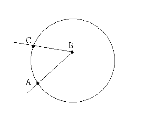
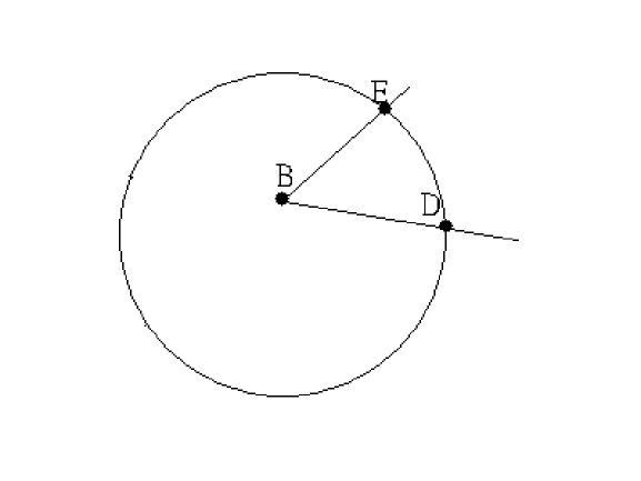
show the result. In Figure 1, there is one random path, from point
to point then from point to point . In Figure 2,
there is one random path, from point to point then from
point to point . The events of these two figures are
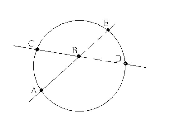
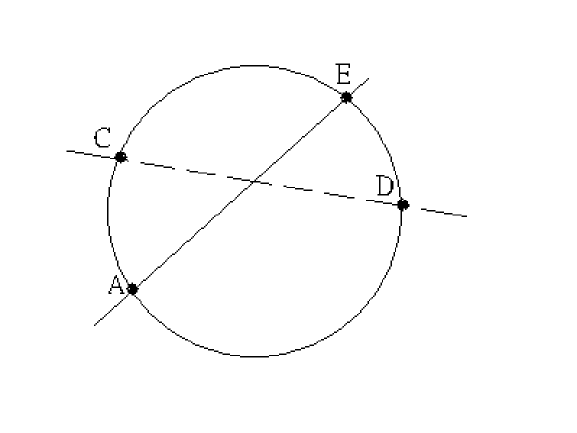
equally likely. In the Figure 3, there are two random paths, one
is the same as in Figure 1 and the other is the same as in Figure
2. In the Figure 4, there are two random paths, one is the path
from point to point then from point to point . and
the other is the path from point to point then from point
to point . Using these facts, these two cases of events and
their associated probabilities, events in Figure 3 and the events
in Figure 4, must be equivalent to each other. These arguments
support that the expectation of random path (Figure 3) is the same
as that of random chords (Figure 4).
The Theoretical Values of
Now, we are going to find the expectation of random chord. Without losing the generality, we solve the two dimensional problems instead of n-dimensional problem. Though there are so called the Bertrand paradox in random chords problem, we are able solve paradox since the results computer simulation will show the correct answer of this paradox. This verifying work could not be done in that time.
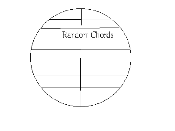
We consider a circle with radius . The set of all chords is well defined. Therefore, we can find the expectation (average) of the lengths of the set of chords. Since the chords are uniformly and randomly distributed in the circle. we can find some subset of these chords by defining a equivalent relation. The parallel relation between chords is a equivalent relation on the set of that chords. The equivalent relation partitions this set into disjoint equivalent classes. Clearly, the expectations of these equivalent classes must be the same one. In the case of finite set, if the mean of all disjoint subsets is the same one, then the set has the same as that of these subsets. Therefore, we will compute the expectation of the random chords in one of these equivalent classes. In figure 5, the measure of the distribution is . Therefore, we have expectation of random chords, ,
. (3)
| (3) |
We interpretate equation (3) as since the diameter is the normal section of the circle. This interpretation can be generalize to higher dimension cases.
From identity (2), we have
| (4) |
where is the volume of the
normal section of and is the boundary area of .
Here, we mean that the sphere contains all its interior points. If
it is necessary, we will use the term the sphere surface which is
to be used in usual sense of mathematician. From equation
(4), we are able to calculate the theoretical values of
all .
Discovery of some sequence
The paper, by H. Chalkley, J. Confield and H. Park, stresses how to estimate the ratio of volume and area. So do their followers’. But our interest is to find the values of . It can be shown that the values of depend on the dimension the space and that the values of are not dependent on the shape or the size of the bounded regions. The ratio of is well known. If we can find the expectation of random chords, then we are able to get the theoretical values of .
From equation (1), We can estimate the value of by computer simulation while the theoretical value of can be obtained by equation . The values of are , , , , …, …, , …
Our approach is to study the related topics rather than to solve this problem separately or independently. In order to convince the readers that the results we obtain are correct and can be verified by computer simulation, the computer programs have been run on PC, DEC VAX 9000, and IBM SP2 for more than 5 years. It is computer that generates a phenomenon which we have never found. From this phenomenon, we try to find some mathematical model to fit it. It is quite natural to generalize the results to Riemannian manifold. And then the sequence , , , ,…,,…, ,…, is discovered. So far, we have found that Kd’s depend on the dimension of the space or manifold only.
It takes time to judge how important the identity , , is, because there are many branches of mathematics such as
geometry, analysis and probability or measure theory, concerning
with this equation . We think that this is a interesting
problem.
We have done the computer simulation of random walk on Riemannian
manifold, the surface of the sphere , . Almost the
same result is obtained. We will organize another paper to show
how to design the computer program for simulating the random walk
on the surface of sphere . We shall simply use Riemannian
manifold in usual sense. In , we are shocked by a
simple example. Let the boundary region be defined on the north
pole of the earth . The region is a circle of which the
center is the north pole and the radius , ,
since , the region becomes a circle on the south
pole. The chord of the circle is defined as the segment of a
geodesic that contains at least one interior point of the circle,
the bounded region. Of course, the two end points must be on the
circle. Let us use the spherical coordinate system, ,
and . Here is constant since we are
studying the problem on . For any , , there is a circle defined on the north pole. The value
of is , that
is, . The value of is , The value of is . Therefore, the value of
or is , . The circle is the north hemisphere of the
earth when . Then the value of is ,
the value of is and the value of or is
. We find this is a circle of which all chords have the
same length, . Since we were confused by this circle, we
have spent more than one year’s time to reinvestigate our
formulation. Finally, we found the result is correct.
References
1. H. Solomon, Geometric Probability (Society for Industrial and Applied Mathematics, Philadelphia, Pennsylvania, 1978), pp. 1-32, 127-172 .
2. H. Chalkley, J. Cornfield, H. Park, A method for estimating volume-surface ratios, Science, 110, pp. 295-297 (1949).
3. C. Kittel AND H. Kroemer, Thermal Physics (W.H. Freeman and Company, San Francisco, ed. 2, 1980), pp. 399-414.
4. R.P. Feynman et al., Lectures on Physics (California Institute of Technology, 1963), vol. 1, section 43-3-section 43-5.
5. K. Stowe , Introduction to Statistical Mechanics and Thermodynamics (John Wiley, New York, 1984), pp. 324-327.
6. Hung-Ming Tsai et al., Estimation of the Mean Speed of Mosquitoes, Science Exhibition, Taichung, Taiwan (1993).
the table of data
| dimension 1 | dimension 2 | dimension 3 | dimension 4 | dimension 5 |
| 0.50065 | 0.313622 | 0.248796 | 0.216937 | 0.188525 |
| 0.4994 | 0.319567 | 0.262792 | 0.211288 | 0.18821 |
| 0.58505 | 0.313033 | 0.251967 | 0.213581 | 0.197106 |
| 0.49935 | 0.319322 | 0.257308 | 0.232106 | 0.185656 |
| 0.49895 | 0.323244 | 0.252587 | 0.214341 | 0.18923 |
| 0.53095 | 0.316656 | 0.245117 | 0.211194 | 0.19041 |
| 0.55985 | 0.346344 | 0.254642 | 0.209172 | 0.195942 |
| 0.50035 | 0.3259 | 0.251117 | 0.21765 | 0.189067 |
| 0.4995 | 0.314611 | 0.255404 | 0.217041 | 0.193394 |
| 0.5001 | 0.314278 | 0.249083 | 0.209794 | 0.188805 |
| 0.4988 | 0.324444 | 0.250887 | 0.211703 | 0.193387 |
| 0.49885 | 0.321067 | 0.255754 | 0.206331 | 0.18697 |
| 0.54215 | 0.3226 | 0.254733 | 0.220672 | 0.190093 |
| 0.4994 | 0.320378 | 0.263854 | 0.212503 | 0.195502 |
| 0.50035 | 0.313078 | 0.253188 | 0.207934 | 0.188976 |
| 0.49935 | 0.321233 | 0.254737 | 0.214747 | 0.196928 |
| 0.50005 | 0.3178 | 0.247129 | 0.210894 | 0.190982 |
| 0.5003 | 0.3166 | 0.254737 | 0.215356 | 0.186613 |
| 0.50065 | 0.349744 | 0.252467 | 0.214447 | 0.195952 |
| 0.4988 | 0.314167 | 0.251663 | 0.212528 | 0.18815 |
| 1/2 | 1/4 | 3/16 | ||
| dimension 6 | dimension 7 | dimension 8 | dimension 9 | dimension 10 |
| 0.171587 | 0.15727 | 0.150828 | 0.141217 | 0.13023 |
| 0.170157 | 0.156205 | 0.146288 | 0.140869 | 0.131315 |
| 0.170313 | 0.157762 | 0.145272 | 0.136662 | 0.126905 |
| 0.172759 | 0.158712 | 0.142739 | 0.137612 | 0.130235 |
| 0.174857 | 0.155061 | 0.144548 | 0.14564 | 0.13146 |
| 0.178097 | 0.155077 | 0.143702 | 0.140506 | 0.130815 |
| 0.170351 | 0.15632 | 0.150119 | 0.134872 | 0.12698 |
| 0.169589 | 0.152943 | 0.147578 | 0.137501 | 0.131175 |
| 0.173221 | 0.154071 | 0.145909 | 0.136983 | 0.125865 |
| 0.176309 | 0.161386 | 0.143639 | 0.13556 | 0.129785 |
| 0.170673 | 0.15788 | 0.146711 | 0.133069 | 0.132895 |
| 0.167793 | 0.157454 | 0.143225 | 0.136452 | 0.12908 |
| 0.169161 | 0.160764 | 0.143214 | 0.140338 | 0.13793 |
| 0.170093 | 0.155816 | 0.144177 | 0.141294 | 0.131325 |
| 0.175531 | 0.153232 | 0.145216 | 0.135168 | 0.12902 |
| 0.169005 | 0.158348 | 0.14707 | 0.13701 | 0.12985 |
| 0.170316 | 0.153707 | 0.14688 | 0.138528 | 0.13025 |
| 0.17744 | 0.158312 | 0.146405 | 0.134812 | 0.138405 |
| 0.17088 | 0.160957 | 0.146869 | 0.13817 | 0.131965 |
| 0.169431 | 0.157529 | 0.147278 | 0.135202 | 0.1304 |
| 5/32 | 35/256 |
The computer program
program sphere
! This main program. id and k are the control variable for
! the dimension of the sace. m is the number
! of partcles. n is the steps of random walk.
dimension x(600100,10),dd(600100,10),dx(10),tow(10),tm(10),tn(10)
open(2,file=”D:forsp41.dat”,status=”unknown”)
rewind(2)
write(2,*)”t=0.01 pro=sp n=1000 4th aprali”
pi=3.1415926
r=1
t=0.01
do id=1,10
ii=id
call brn(ii,a,ad)
nn=a*1.15**id
n=1000*nn
m=1000*nn
do k=1,10
s=0
ss=0
! The m number of particles is uniformly distributed.
! The partcles is generated uniforly in the general interval.
! The method of rejction is used to obtain the desired results.
do i=1,m
100 rs=0
do j=1,id
call random_number(xZ)
x(i,j)=2*xz-1
rs=x(i,j)**2+rs
end do
r1=sqrt(rs)
if (r1 .GE. r)go to 100
end do
do l1=1,n
ss1=0
! The directions of next step are generated.
do i=1,m
call rt(dx,id)
do j=1,id
dd(i,j)=dx(j)
end do
end do
! The postions of m partcles are updated.
! Of course, the counters s and ss1 are used to
! count the number of partcles that hit the boundary.
! The technique for using two counter s and ss1 insure
! the sum is correct. That is, sss1=ss1+1 is not correc
! counter, when the content is very large.
do i=1,m
do j=1,id
dx(j)=dd(i,j)
tow(j)=x(i,j)
x(i,j)=x(i,j)+t*dx(j)
tn(j)=x(i,j)
end do
rs=0
do j=1,id
rs=x(i,j)**2+rs
end do
r1=sqrt(rs)
if(r1 .LT. r) go to 300
call tt(tow,tn,r,dx,id,t)
do j=1,id
x(i,j)=tn(j)
dd(i,j)=dx(j)
end do
s=s+1
ss1=ss1+1
300 end do
ss=ss+ss1
ss1=0
end do
! The theoretical value of K, ty , is computed.
ii=id
call voa(ii,a,ad)
tx=n
sm=m
b=a*id
tk=ss/(sm*b*tx*t)*a
ty=ad/b
! The computer simulation of K is tk.
write(2,*)tk,ty
write(*,*)tk,ty
end do
end do
close(2)
stop
end
subroutine tt(tow,tn,r,dx,id,t)
! In this subprogram, the new postion is determined
! when the partcle collides the boundary of sphere.
! The elastic reflection is computed. A simple property is used.
! That is, any position, including on the boundary, of the particle is vector which is
! perpendicular to the (tangent of )boundary
dimension tow(10),tn(10),dx(10),f(10),g(10),h(10)
ap=0
pl=0
do j=1,id
ap=ap+dx(j)*tow(j)
pl=pl+tow(j)**2
end do
tp=-ap+sqrt(ap**2+1-pl)
pr=0
pr1=0
do j=1,id
f(j)=tow(j)+tp*dx(j)
pr=pr+(tn(j)-f(j))*f(j)
pr1=pr1+dx(j)*f(j)
end do
dl=0
do j=1,id
tn(j)=tn(j)-2*pr*f(j)
dx(j)=dx(j)-2*pr1*dx(j)
dl=dl+dx(j)**2
end do
dl=1.0/sqrt(dl)
do j=1,id
dx(j)=dx(j)*dl
end do
return
end
subroutine rt(dx,id)
! In this subprogram a random unit vector is generated for
! direction of next step random walking.
dimension dx(10)
100 tl=0
do j=1,id
call random_number(xz)
dx(j)=2*xz-1
tl=tl+dx(j)**2
end do
if(tl .EQ. 0) go to 100
tl=sqrt(tl)
if(tl .GT. 1) go to 100
tl=1.0/tl
do j=1,id
dx(j)=dx(j)*tl
end do
return
end
subroutine voa(ii,a,ad)
! In the subprogram, both the volumes of unit sphere and the normal section
! section of the unit sphere are computed. For example, if input ii=3,
! then output a is the volume of three dimensional unit sphere and
! the other output ad is the area of a unit two dimensinal sphere, the disk.
ii=ii-1
call brn(ii,a,ad)
ad=a
ii=ii+1
call brn(ii,a,ad)
return
end
subroutine brn(ii,a,ad)
! In this subprogram, the volume of unit sphere is computed
! The parameter ii is the dimension, the parameter a is ouput and
! the parameter ad is a redunduncy
in=ii/2
in=ii-2*in+1
if (in .EQ. 2)go to 400
f=1
ls=ii/2
do j= 1,ls
f=f*j
end do
a=3.1415926**ls/f
go to 500
400 f=1
do j=1,ii
f=f*j
end do
l1=(ii-1)/2
f1=1
do j=1,l1
f1=f1*j
end do
a=3.1415926**l1*2**ii*f1/f
500 return
end