Static Interactions of $U(N)$ non-Abelian Vortices

Abstract

Interactions between non-BPS non-Abelian vortices are studied in non-Abelian $U(1)\times SU(N)$ extensions of the Abelian-Higgs model in four dimensions. In addition to the usual type I/II Abelian superconductors, we find other two new regimes: type I^∗/II^∗.

1 Introduction

Recently, a new type of BPS vortex was found in $U(N)$ gauge theories [1, 2]. This is called non-Abelian vortex and carries the non-Abelian charge ${\bf C}P^{N-1}=\frac{SU(N)_{{\rm C}+{\rm F}}}{SU(N-1)_{{\rm C}+{\rm F}}\times U(1)_{{\rm C}+{\rm F}}}$. Readers can find good reviews in [3, 4] and references of related works therein. In this talk we are interested in studying interactions between non-Abelian vortices which are non-BPS. The non-BPS vortices are more natural than BPS ones in a sense that the BPS always requires a fine tuning or supersymmetry. It is well known that ANO vortices [5, 6] in the type I system feel an attractive force while those in the type II model feel a repulsive force [7, 8, 9, 10]. Specifically we are interested in the interactions between vortices with different internal orientations, which is the distinct feature from the ANO case [11].

This talk is based on [12] in collaboration with R.Auzzi and W.Vince.

2 The model

2.1 A fine-tuned model

We start with non-Abelian, $U(N)$, extension of the Abelian-Higgs model

$${\cal L}={\rm Tr}\left[-\frac{1}{2e^{2}}F_{\mu\nu}F^{\mu\nu}+\mathcal{D}_{\mu}H(\mathcal{D}^{\mu}H)^{\dagger}-{\frac{\lambda^{2}\,e^{2}}{4}}\left(v^{2}{\bf 1}_{N}-HH^{\dagger}\right)^{2}\right].$$ (1)

Here, for simplicity we take the same gauge coupling $e$ for both the $U(1)$ and $SU(N)$ groups, while $\lambda^{2}\,e^{2}/4$ is a scalar coupling and $v$ ($>0$) determines the Higgs VEV. $H$ is $N$ Higgs fields in the fundamental representation of $U(N)$. The Higgs vacuum of the model is given by $HH^{\dagger}=v^{2}{\bf 1}_{N}$. It breaks completely the gauge symmetry, although a global color-flavor locking symmetry $SU(N)_{\rm C+F}$ is preserved

$$H\to U_{\rm G}HU_{\rm F},\quad U_{\rm G}=U_{\rm F}^{\dagger},\quad U_{\rm G}\in SU(N)_{\rm G},\ U_{\rm F}\in SU(N)_{\rm F}.$$ (2)

The trace part ${\rm Tr}H$ is a singlet under the color-flavor group and the traceless parts are in the adjoint representation. The $U(1)$ and the $SU(N)$ gauge vector bosons have both the same mass $M_{U(1)}=M_{SU(N)}=e\,v$. The $N^{2}$ real scalar fields in $H$ are eaten by the gauge bosons and the other $N^{2}$ (one singlet and the rest adjoint) have same masses $M_{\rm s}=M_{\rm ad}=\lambda\,e\,v$. The critical coupling $\lambda=1$ (BPS) allows an $\mathcal{N}=2$ supersymmetric extension.

2.2 Models with general couplings

A generalization of (1) is to consider different gauge couplings, $e$ for the $U(1)$ part and $g$ for the $SU(N)$ part, and a general quartic scalar potential

$${\cal L}={\rm Tr}\left[-\frac{1}{2g^{2}}\hat{F}_{\mu\nu}\hat{F}^{\mu\nu}-\frac{1}{2e^{2}}f_{\mu\nu}f^{\mu\nu}+\mathcal{D}_{\mu}H(\mathcal{D}^{\mu}H)^{\dagger}\right]-V,$$ (3)

where we have defined $\hat{F}_{\mu\nu}=\sum_{A=1}^{N^{2}-1}F_{\mu\nu}^{A}T_{A}$ and $f_{\mu\nu}=F_{\mu\nu}^{0}T^{0}$ with ${\rm Tr}(T^{A}T^{B})=\delta^{AB}/2$ and $T^{0}={\bf 1}/\sqrt{2N}$ The scalar potential is:

$$V=\frac{\lambda_{g}^{2}g^{2}}{4}{\rm Tr}\hat{X}^{2}+\frac{\lambda_{e}^{2}e^{2}}{4}{\rm Tr}\left(X^{0}T^{0}-v^{2}{\bf 1}_{N}\right)^{2},$$ (4)

where $HH^{\dagger}=X^{0}T^{0}+\hat{X}$ and $\hat{X}=2\sum_{A=1}^{N^{2}-1}\left(H^{i\dagger}T^{A}H_{i}\right)T^{A}$. The symmetries is same as the previous fine-tuned model (1). In this model, the $U(1)$ and the $SU(N)$ vector bosons have different masses $M_{U(1)}=e\,v,\ M_{SU(N)}=g\,v.$ Moreover, the singlet part of $H$ has a mass $M_{\rm s}$ different from that of the adjoint part $M_{\rm ad}$ as $M_{\rm s}=\lambda_{e}\,e\,v,\ M_{\rm ad}=\lambda_{g}\,g\,v$. For the critical values $\lambda_{e}=\lambda_{g}=1$, the Lagrangian again allows an $\mathcal{N}=2$ susy extension.

2.3 Vortex equations in the fine-tuned model

Let us make the following rescaling of fields and coordinates:

$$H\rightarrow vH,\quad W_{\mu}\rightarrow evW_{\mu},\quad x_{\mu}\rightarrow\frac{x_{\mu}}{ev}.$$ (5)

The masses of vector and scalar bosons are rescaled to

$$M_{U(1)}=M_{SU(N)}=1,\qquad M_{\rm s}=M_{\rm ad}=\lambda.$$ (6)

In order to construct non-BPS non-Abelian vortex solutions, we have to solve the equation of motion derived from the Lagrangian (1),

$$\mathcal{D}_{\mu}F^{\mu\nu}-\frac{i}{2}\left[H(\mathcal{D}^{\nu}H)^{\dagger}-(\mathcal{D}^{\nu}H)H^{\dagger}\right]=0,$$ (7)

$$\mathcal{D}_{\mu}\mathcal{D}^{\mu}H+\frac{\lambda^{2}}{4}\left(1-HH^{\dagger}\right)H=0.$$ (8)

From now on, we restrict ourselves to static configurations depending only on the coordinates $x^{1},x^{2}$. Here we introduce a complex notation $z=x^{1}+ix^{2},\partial=\frac{\partial_{1}-i\partial_{2}}{2},\ W=\frac{W_{1}-iW_{2}}{2},\ \mathcal{D}=\frac{\mathcal{D}_{1}-i\mathcal{D}_{2}}{2}=\partial+iW$. Instead of the equation of motions itself, it might be better to study gauge invariant quantities. For that purpose let us define

$$\bar{W}(z,\bar{z})=-iS^{-1}(z,\bar{z})\bar{\partial}S(z,\bar{z}),\quad H(z,\bar{z})=S^{-1}(z,\bar{z})\tilde{H}(z,\bar{z}),$$ (9)

where $S$ takes values in $GL(N,{\bf C})$ and it is in the fundamental representation of $U(N)$ while the gauge singlet $\tilde{H}$ is an $N\times N$ complex matrix. There is an equivalence relation $(S,\tilde{H})\sim(V(z)S,V(z)\tilde{H})$, where $V(z)$ is a holomorphic $GL(N,{\bf C})$ matrix with respect to $z$. The gauge group $U(N)$ and the flavor symmetry act as follows

$$S(z,\bar{z})\to U_{\rm G}S(z,\bar{z}),\quad H_{0}(z)\to H_{0}(z)U_{\rm F}.$$ (10)

An important gauge invariant quantity is now constructed as

$$\Omega(z,\bar{z})\equiv S(z,\bar{z})S(z,\bar{z})^{\dagger}.$$ (11)

With respect to the gauge invariant objects, the equations of motion are

$$4\bar{\partial}^{2}\left(\Omega\partial\Omega^{-1}\right)-\tilde{H}\bar{\partial}\left(\tilde{H}^{\dagger}\Omega^{-1}\right)+\bar{\partial}\tilde{H}\tilde{H}^{\dagger}\Omega^{-1}=0,\qquad\quad$$ (12)

$$\Omega\partial\left(\Omega^{-1}\bar{\partial}\tilde{H}\right)+\bar{\partial}\left(\Omega\partial\left(\Omega^{-1}\tilde{H}\right)\right)+\frac{\lambda^{2}}{4}\left(\Omega-\tilde{H}\tilde{H}^{\dagger}\right)\Omega^{-1}\tilde{H}=0.$$ (13)

These equations must be solved with the boundary conditions for $k$ vortices $\det\tilde{H}\rightarrow z^{k},\ \Omega\rightarrow\tilde{H}\tilde{H}^{\dagger}$ as $z\rightarrow\infty$.

2.4 BPS Limit

For the later convenience, let us see the BPS limit $\lambda\to 1$. It can be done by just taking a holomorphic function $\tilde{H}$ with respect to $z$ as

$$\tilde{H}=H_{0}(z).$$ (14)

Then the equations (12) and (13) reduce to the single matrix equation

$$\bar{\partial}\left(\Omega\partial\Omega^{-1}\right)+\frac{1}{4}\left({\bf 1}-H_{0}H_{0}^{\dagger}\Omega^{-1}\right)=0.$$ (15)

This is the master equation for the BPS non-Abelian vortex and the holomorphic matrix $H_{0}(z)$ is called the moduli matrix [13, 4]. All the complex parameters contained in the moduli matrix are moduli of the BPS vortices. For example, the position of the vortices can be read from the moduli matrix as zeros of its determinant $\det H_{0}(z_{i})=0$. Furthermore, the number of vortices (the units of magnetic flux of the configuration) corresponds to the degree of $\det H_{0}(z)$ as a polynomial with respect to $z$. The classification of the moduli matrix for the BPS vortices is given in Ref. [13, 4].

Consider $U(2)$ gauge theory. The minimal vortex is generated by

$$H_{0}^{(1,0)}=\left(\begin{array}[]{cc}z-z_{0}&0\\ -b^{\prime}&1\end{array}\right),\qquad H_{0}^{(0,1)}=\left(\begin{array}[]{cc}1&-b\\ 0&z-z_{0}\end{array}\right).$$ (20)

$z_{0}$ corresponds to the position of the vortex and $b$ and $b^{\prime}$ are the internal orientation. One can extract the orientation as the null eigenvector of $H_{0}(z)$ at the vortex position $z=z_{0}$ as

$$\vec{\phi}^{~{}(1,0)}=\left(\begin{array}[]{c}1\\ b^{\prime}\end{array}\right)\quad\sim\quad\vec{\phi}^{~{}(0,1)}=\left(\begin{array}[]{c}b\\ 1\end{array}\right).$$ (25)

Here “$\sim$” stands for an identification up to complex non zero factors: $\vec{\phi}\sim\lambda\vec{\phi}$, $\lambda\in{\bf C}^{*}$, so that we have found ${\bf C}P^{1}$ [13, 4]. We call two non-Abelian vortices with equal orientational vectors parallel, while orthogonal orientational vectors anti-parallel.

Arbitrary two vortices (the center of mass is fixed to be zero and the overall orientaion is fixed) is given by

$$H_{0\ {\rm red}}^{(1,1)}\equiv\left(\begin{array}[]{cc}z-z_{0}&-\eta\\ 0&z+z_{0}\end{array}\right).$$ (28)

The orientational vectors are then of the form

$$\vec{\phi}^{~{}(1,1)}_{1}\big{|}_{z=z_{0}}=\left(\begin{array}[]{c}1\\ 0\end{array}\right),\qquad\vec{\phi}^{~{}(1,1)}_{2}\big{|}_{z=-z_{0}}=\left(\begin{array}[]{c}\eta\\ -2z_{0}\end{array}\right).$$ (33)

3 Vortex interaction in the fine-tuned model

3.1 $(k_{1},k_{2})$ coincident vortices

The minimal winding solution in the non-Abelian gauge theory is a mere embedding of the ANO solution into the non-Abelian theory. Embedding is also useful for another simple non-BPS configurations. Let us start with the moduli matrix for a configuration of $k$ coincident vortices. The axial symmetry allows a reasonable ansatz for $\Omega$ and $\tilde{H}$

$$\Omega^{(0,1)}=\left(\begin{array}[]{cc}1&0\\ 0&w(r)\end{array}\right),\qquad\tilde{H}^{(0,1)}=\left(\begin{array}[]{cc}1&0\\ 0&f(r)z^{k}\end{array}\right).$$ (38)

We call this “$(0,k)$-vortex”. When $k\geq 2$, it is possible that the ansatz (38) does not give the true solution (minimum of the energy) of the equations of motion (12) and (13). This is because there could be repulsive forces between the vortices. With ansatz (38) we fix the positions of all the vortices at the origin by hand. The master equation (15) is nevertheless still useful to investigate the interactions between two vortices. The results are listed in Table 1.

$\lambda$ $k=1$ $k=2$ 0.8 0.91231 1.77407 0.9 0.95737 1.88936 1 1.00000 2.00000 1.1 1.04053 2.10655 1.2 1.07922 2.20944

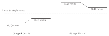
Figure 1: Spectrum of the $(0,2)$ and $(1,1)$ coincident vortices.

For $\lambda=1$, the masses are identical to integer values, up to $10^{-5}$ order, which are nothing but the winding number of the vortices.

There is another type of composite configuration which can easily be analyzed numerically

$$\Omega^{(1,1)}=\left(\begin{array}[]{cc}w_{1}(r)&0\\ 0&w_{2}(r)\end{array}\right),\qquad\tilde{H}^{(1,1)}=\left(\begin{array}[]{cc}f_{1}(r)z^{k_{1}}&0\\ 0&f_{2}(r)z^{k_{2}}\end{array}\right).$$ (43)

This ansatz corresponds to a configuration with $k_{1}$ composite vortices which wind in the first diagonal $U(1)$ subgroup of $U(2)$ and with $k_{2}$ coincident vortices that wind the second diagonal $U(1)$ subgroup. We refer to these as a “$(k_{1},k_{2})$-vortex”. The mass of a $(k_{1},k_{2})$-vortex is thus the sum of the mass of the $(k_{1},0)$-vortex and that of the $(0,k_{2})$-vortex.

We call the non-Abelian vortices in the fine-tuned model for $\lambda<1$ type I, while they will be called type II for $\lambda>1$. From Fig. 1, we can see that in the type I case, the $(0,2)$-vortex is energetically preferred to the $(1,1)$-vortex, while in type II case the $(1,1)$-vortex is preferred. If the two vortices are separated sufficiently, regardless of their orientations, the mass of two well separated vortices is twice that of the single vortex. This mass is equal to the mass of the $(1,1)$-vortex.

3.2 Effective potential for coincident vortices

The dynamics of BPS solitons can be investigated by the so-called moduli approximation [14]. The effective action is a massless non-linear sigma model whose target space is the moduli space. If the coupling constant $\lambda$ is close to the BPS limit $\lambda=1$, we can still use the moduli approximation, to investigate dynamics of the non-BPS non-Abelian vortices by adding a potential of order $|1-\lambda^{2}|\ll 1$. To this end, we write the Lagrangian

$$\tilde{\cal L}=\tilde{\cal L}_{\rm BPS}+\frac{(\lambda^{2}-1)}{4}\left({\bf 1}_{N}-HH^{\dagger}\right)^{2}.$$ (44)

We get non-BPS corrections of order $O(\lambda^{2}-1)$ by putting BPS solutions into Eq. (44). The energy functional thus takes the following form

$${\cal E}=2+(\lambda^{2}-1){\cal V},\quad{\cal V}=\frac{1}{8\pi}\int dx^{1}dx^{2}\ {\rm Tr}\left({\bf 1}-\left|H_{\rm BPS}(\varphi_{i})\right|^{2}\right)^{2}$$ (45)

where $H_{\rm BPS}(\varphi_{i})$ stands for the BPS solution. We have defined a reduced effective potential ${\cal V}$ which is independent of $\lambda$. The first term corresponds to the mass of two BPS vortices and the second term is the deviation from the BPS solutions which is nothing but the effective potential we want.

To have the effective potential on the moduli space of coincident vortices, it suffices to consider only the matrix (28) with turning off the relative distance $z_{0}$. In order to evaluate it, we need to solve the BPS equations with an intermediate value of $\eta$. Because of the axial symmetry and the boundary condition at infinity $\Omega\rightarrow H_{0}(z)H_{0}^{\dagger}(\bar{z})$, we can make an ansatz

$$\Omega^{(1,1)}=\left(\begin{array}[]{cc}w_{1}(r)&-\eta e^{-i\theta}w_{2}(r)\\ -\eta e^{i\theta}w_{2}(r)&w_{3}(r)\end{array}\right).$$ (48)

The advantage of the moduli matrix formalism is that only three functions $w_{i}(r)$ are needed and the formalism itself is gauge invariant. The effective potential can be obtained by plugging numerical solutions into Eq. (45). The result is shown in Fig. 2.

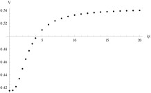
Figure 2: Numerical plots of the effective reduced potential ${\cal V}(|\eta|)$.

The type II effective potential has the same qualitative behavior as showed in the figure. It has a minimum at $|\eta|=0$. This matches the previous result that the $(1,1)$-vortex is energetically preferred to the $(2,0)$-vortex. The type I effective potential can be obtained just by flipping the overall sign of that of the type II case. Then the effective potential always takes a negative value, which is consistent with the fact that the masses of the type I vortices are less than that of the BPS vortices. Contrary to the type II case, the type I potential has a minimum at $|\eta|=\infty$, so that the $(2,0)$-vortex is preferred to the $(1,1)$ vortex.

3.3 Interaction at generic vortex separation

Next we go on investigating the interactions of non-Abelian vortices in the $U(2)$ gauge group at generic distances. We will again use the moduli space approximation. The generic configurations are described by the moduli matrices in Eq. (28). By putting the two vortices on the real axis, we can reduce $z_{0}$ to a real parameter $d$. So $2d$ is the relative distance and $\eta$ the relative orientation. Now let us study the effective potential as function of $\eta$ and $d$. As before, we first need the numerical solution to the BPS master equation. Despite the great complexity by broken axial symmetry, the moduli matrix formalism is a powerful tool and the relaxation method is very effective to solve the problem. Once we get the numerical solution, the effective potential is obtained by plugging them into Eq. (45), see Fig. 3. It for the type II has the same shape, up to a small positive factor ($\lambda^{2}-1$). The potential forms a hill whose top is at $(d,|\eta|)=(0,\infty)$. It clearly shows that two vortices feel repulsive forces, in both the real and internal space, for every distance and relative orientation. The minima of the potential has a flat direction along the $d$-axis where the orientations are anti-parallel $(\eta=0)$ and along the $\eta$ axis at infinite distance $(d=\infty)$. Therefore the anti-parallel vortices do not interact.

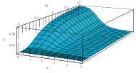
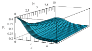
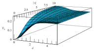
Figure 3: Left panel is the effective potential ${\cal V}(\eta,d)$. The Abelian potential ${\cal V}_{e}$ (middle) and the non-Abelian potential ${\cal V}_{g}$ (right) for $\gamma=1$.

In the type I case ($\lambda<1$) the effective potential is upside-down of that of the type II case. There is unique minimum of the potential at $(d,|\eta|)=(0,\infty)$. This means that attractive force works not only for the distance in real space but also among the internal orientations.

4 Vortices with generic couplings

In this section we sutudy the general model defined in Eqs. (3) and (4). We have three effective couplings $\gamma=g/e,\lambda_{e},\lambda_{g}$ after the rescaling (5). The masses of particles are rescaled as

$$M_{U(1)}=1,\quad M_{SU(N)}=\gamma,\quad M_{\rm s}=\lambda_{e},\quad M_{\rm ad}=\gamma\lambda_{g}.$$ (49)

In order to find the effective potential on the moduli space as before, we need to clarify BPS configurations. The moduli matrix in (14) is still valid, while the master equation (15) get a modification

$$4\bar{\partial}\left(\Omega\partial\Omega^{-1}\right)=\Omega_{0}\Omega^{-1}-{\bf 1}_{N}+(\gamma^{2}-1)\left(\Omega_{0}\Omega^{-1}-\frac{{\rm Tr}\left(\Omega_{0}\Omega^{-1}\right)}{N}{\bf 1}_{N}\right)$$ (50)

where $\Omega=SS^{\dagger}$ is same as before and $\Omega_{0}\equiv H_{0}H_{0}^{\dagger}$. It turns out that the effective potential consists of the Abelian and the non-Abelian potentials

$${\cal V}_{e}(\eta,d;\gamma)=\int d\tilde{x}^{2}\ {\rm Tr}(F_{12}^{0}T^{0})^{2},\quad{\cal V}_{g}(\eta,d;\gamma)=\int d\tilde{x}^{2}\ {\rm Tr}(\hat{F}_{12})^{2}.$$ (51)

The true potential is a linear combination of them

$$V(\eta,d;\gamma,\lambda_{e},\lambda_{g})=(\lambda_{e}^{2}-1){\cal V}_{e}(\eta,d;\gamma)+\frac{\lambda_{g}^{2}-1}{\gamma^{2}}{\cal V}_{g}(\eta,d;\gamma).$$ (52)

4.1 Equal gauge coupling $\gamma=1$ revisited

The effective potential with $\gamma=1$ and $\lambda=\lambda_{g}=\lambda_{e}$ in the left panel of Fig. 3 should be now decomposed in the two potentials, see the middle and the right panels in Fig. 3. In the case with $\lambda_{e}^{2}-1>0$ and $\lambda_{g}^{2}-1>0$, the effective potential will have the same qualitative behaviors like the reduced potentials in the Figs. 3. The figures shows how ${\cal V}_{e}$ and ${\cal V}_{g}$ behaves very differently. In particular, the Abelian potential is always repulsive, both in the real and internal space. The non-Abelian potential is on the contrary sensitive on the orientations. Fig. 3 shows that it is repulsive for parallel vortices while it is attractive for anti-parallel ones. When the two scalar couplings are equal, $\lambda_{e}^{2}=\lambda_{g}^{2}$, the two potentials exactly cancel for anti-parallel vortices.

Of course, the true effective potential depends on $\lambda_{e}$ and $\lambda_{g}$ through the combination in Eq. (52). This indicates the interaction between non-Abelian vortices is quite rich in comparison with that of the ANO vortices.

4.2 Different gauge coupling $\gamma\neq 1$

We now consider interactions between non-Abelian vortices with different gauge coupling $e\neq g$ ($\gamma\neq 1$). In Figs. 5 and 5 we show two numerical examples for the reduced effective potentials ${\cal V}_{e}$, ${\cal V}_{g}$ given in Eq. (51).

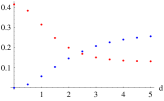
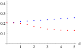
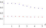
anti-parallel ($\eta=0$)		intermediate ($\eta=4$)		parallel ($\eta=\infty$)

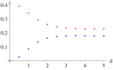
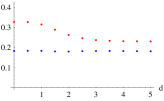
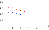
Figure 4: Effective potential with $\gamma=1/2$ vs. separation. (red, blue) = (${\cal V}_{e}$, ${\cal V}_{g}$).

anti-parallel ($\eta=0$)		intermediate ($\eta=4$)		parallel ($\eta=\infty$)

Figure 5: Effective potential with $\gamma=1.3$ vs. separation. (red, blue) = (${\cal V}_{e}$, ${\cal V}_{g}$).

These show that the qualitative features of ${\cal V}_{e}$ and ${\cal V}_{g}$ are basically the same as what is discussed in the equal gauge coupling case $(\gamma=1)$. The true effective potential in Eq. (52) depends on the three parameters $\gamma$, $\lambda_{e}$ and $\lambda_{g}$. We can have potentials which develop a global minimum at some finite non zero distance, see Fig. 6

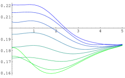
Figure 6: $\gamma=1/2$, $\lambda_{e}=1.2$, $\lambda_{g}=1.06$: From $\eta=0$ (green) to $\eta=7$ (blue) with $d=0\sim 5$ for each $\eta$.

The figure shows the presence of a minimum around $d\sim 2.$ This kind of behavior have not been found for the ANO type I/II vortices and the possibility of bounded vortices really results from the non-Abelian symmetry.

5 Interaction at large vortex separation

5.1 Vortices in fine-tuned models $e=g$ and $\lambda_{e}=\lambda_{g}$

We study an asymptotic forces between vortices at large separation, following Refs. [10]. We need to find asymptotic behaviors around $(1,0)$-vortex

$$H_{0}(z)^{(1,0)}=\left(\begin{array}[]{cc}z&0\\ 0&1\end{array}\right),\qquad\vec{\phi}_{1}^{(1,0)}=\left(\begin{array}[]{cc}1\\ 0\end{array}\right).$$ (57)

We are lead to the well known asymptotic behavior of the ANO vortex

$$H_{[1,1]}=\left(1+\frac{q}{2\pi}K_{0}(\lambda r)\right)e^{i\theta},\quad\bar{W}_{[1,1]}=-\frac{i}{2}\left(\frac{1}{r}-\frac{m}{2\pi}K_{1}(r)\right)e^{i\theta},$$ (58)

where $K_{1}\equiv-K^{\prime}_{0}$ and we have defined $H_{[1,1]}$ and $\bar{W}_{[1,1]}$ as $[1,1]$ elements of $H$ and $\bar{W}$ in Eq. (9) with the $k=1$ ansatz (38).

Next we treat the vortices as point particles in a linear field theory coupled with a scalar source $\rho$ and a vector current $j_{\mu}$. To linearize the Yang-Mills-Higgs Lagrangian, we choose a gauge such that the Higgs fields is given by hermitian matrix $H={\bf 1}_{2}+\frac{1}{2}h^{i}\sigma_{i},\ W_{\mu}=\frac{1}{2}w_{\mu}^{i}\sigma_{i}$ with $\sigma=({\bf 1}_{2},\vec{\sigma})$. with all $h^{a},w_{\mu}^{a}$ are real. Then the quadratic part of the Lagrangian is

$${\cal L}^{(2)}_{\rm free}=\sum_{a=0}^{3}\left[-\frac{1}{4}f_{\mu\nu}^{a}f^{a\mu\nu}+\frac{1}{2}w^{a}_{\mu}w^{a\mu}+\frac{1}{2}\partial_{\mu}h^{a}\partial^{\mu}h^{a}-\frac{\lambda^{2}}{2}(h^{a})^{2}\right]$$ (59)

with $f_{\mu\nu}^{a}\equiv\partial_{\mu}w^{a}_{\nu}-\partial_{\nu}w^{a}_{\mu}$. We also take into account the external source terms to realize the point vortex

$${\cal L}_{\rm source}=\sum_{a=0}^{3}\left[\rho^{a}h^{a}-j_{\mu}^{a}w^{a\mu}\right].$$ (60)

The scalar and the vector sources should be determined so that the asymptotic behavior of the fields in Eq. (58) are replicated. The solution of the equation of motion is

$$h^{0}=h^{3}=\frac{q}{2\pi}K_{0}(\lambda r), \ \rho^{0}=\rho^{3}=q\delta(r),$$

$${\bf w}^{0}={\bf w}^{3}=-\frac{m}{2\pi}\hat{\bf k}\times\nabla K_{0}(r), \ {\bf j}^{0}={\bf j}^{3}=-m\hat{\bf k}\times\nabla\delta(r)$$ (61)

where $\hat{\bf k}$ is a spatial fictitious unit vector along the vortex world-volume. The vortex configuration with general orientation is also treated easily, since the origin of the orientation is the Nambu-Goldstone mode associated with the broken $SU(2)$ color-flavor symmetry $H_{0}\to H_{0}(z)^{(1,0)}U_{\rm F},\ \vec{\phi}_{2}=U_{\rm F}^{\dagger}\vec{\phi}_{1}^{(1,0)}$. The interaction between a vortex at ${\bf x}={\bf x}_{1}$ with the orientation $\vec{\phi}_{1}$ and another vortex at ${\bf x}={\bf x}_{2}$ with the orientation $\vec{\phi}_{2}$ is given through the source term and is summarized as

$$V_{\rm int}=-\frac{\left|{\vec{\phi}}^{\dagger}_{1}{\vec{\phi}}_{2}\right|^{2}}{\left|{\vec{\phi}}_{1}\right|^{2}\left|{\vec{\phi}}_{2}\right|^{2}}\left(\frac{q^{2}}{2\pi}K_{0}(\lambda r)-\frac{m^{2}}{2\pi}K_{0}(r)\right),$$ (62)

where $r\equiv|{\bf x}_{1}-{\bf x}_{2}|\gg 1$. When two vortices have parallel orientations, this potential becomes that of two ANO vortices [10]. On the other hand, the potential vanishes when their orientations are anti-parallel. This agrees with the numerical result found in the previous sections. In the BPS limit $\lambda=1$ ($q=m$), the interaction becomes precisely zero.

5.2 Vortices with general couplings

It is quite straightforward to generalize the results of the previous section to the case of generic couplings. We find the total potential $V_{\rm int}$

$$V_{\rm int} = \frac{1}{2}\left(-\frac{(q^{0})^{2}}{2\pi}K_{0}(\lambda_{e}r)+\frac{(m^{0})^{2}}{2\pi}K_{0}(r)\right)$$ (63)

$$+ \left(\frac{\left|{\vec{\phi}}^{\dagger}_{1}{\vec{\phi}}_{2}\right|^{2}}{\left|{\vec{\phi}}_{1}\right|^{2}\left|{\vec{\phi}}_{2}\right|^{2}}-\frac{1}{2}\right)\left(-\frac{(q^{3})^{2}}{2\pi}K_{0}(\lambda_{g}\gamma r)+\frac{(m^{3})^{2}}{2\pi}K_{0}(\gamma r)\right).$$

At large distance, the interactions between vortices are dominated by the particles with the lowest mass $M_{\rm low}$. There are four possible regimes $V_{\rm int}=$

$$\left\{\begin{array}[]{ccll}-\frac{(q^{0})^{2}}{4\pi}\sqrt{\frac{\pi}{2\lambda_{e}r}}e^{-\lambda_{e}r}&{\rm for}&M_{\rm low}=M_{\rm s},&{\rm Type}\,{\rm I}\\ -\left(\frac{\left|{\vec{\phi}}^{\dagger}_{1}{\vec{\phi}}_{2}\right|^{2}}{\left|{\vec{\phi}}_{1}\right|^{2}\left|{\vec{\phi}}_{2}\right|^{2}}-\frac{1}{2}\right)\frac{(q^{3})^{2}}{2\pi}\sqrt{\frac{\pi}{2\lambda_{g}\gamma r}}e^{-\lambda_{g}\gamma r}&{\rm for}&M_{\rm low}=M_{\rm ad},&{\rm Type}\,{\rm I}^{*}\\ \frac{(m^{0})^{2}}{4\pi}\sqrt{\frac{\pi}{2r}}e^{-r}&{\rm for}&M_{\rm low}=M_{U(1)},&{\rm Type}\,{\rm II}\\ \left(\frac{\left|{\vec{\phi}}^{\dagger}_{1}{\vec{\phi}}_{2}\right|^{2}}{\left|{\vec{\phi}}_{1}\right|^{2}\left|{\vec{\phi}}_{2}\right|^{2}}-\frac{1}{2}\right)\frac{(m^{3})^{2}}{2\pi}\sqrt{\frac{\pi}{2\gamma r}}e^{-\gamma r}&{\rm for}&M_{\rm low}=M_{SU(2)},&{\rm Type}\,{\rm II}^{*}\end{array}\right.,$$ (68)

because of $K_{0}(\lambda r)\sim\sqrt{\pi/2\lambda r}e^{-\lambda r}$. This generalizes the type I/II classification of Abelian superconductors. We have found two new categories, called type I^∗ and type II^∗, in which the force can be attractive or repulsive depending on the relative orientation. In the type I^∗ case the forces between parallel vortices are attractive while anti-parallel vortices repel each other. The type II^∗ vortices feel opposite forces to the type I^∗. The result in Eq. (68) is easily extended to the general case of $U(1)\times SU(N)$. This can be done by just thinking of the orientation vectors $\vec{\phi}$ as taking values in ${\bf C}P^{N-1}$.

It may be interesting to compare these results with the recently studied asymptotic interactions between non-BPS non-Abelian global vortices [15].

References

- [1] A. Hanany and D. Tong, JHEP 0307 (2003) 037
- [2] R. Auzzi, S. Bolognesi, J. Evslin, K. Konishi and A. Yung, Nucl. Phys. B 673 (2003) 187
- [3] D. Tong, arXiv:hep-th/0509216; K. Konishi, arXiv:hep-th/0702102; M. Shifman and A. Yung, arXiv:hep-th/0703267.
- [4] M. Eto, Y. Isozumi, M. Nitta, K. Ohashi and N. Sakai, J. Phys. A 39 (2006) R315
- [5] A. A. Abrikosov, Sov. Phys. JETP 5 (1957) 1174 [Zh. Eksp. Teor. Fiz. 32 (1957) 1442].
- [6] H. B. Nielsen and P. Olesen, Nucl. Phys. B61 (1973) 45.
- [7] S. Gustafson and I. M. Sigal, Commun. Math. Phys. 212, 257 (2000).
- [8] L. Jacobs and C. Rebbi, Phys. Rev. B 19, 4486 (1979); K. J. M. Moriarty, E. Myers and C. Rebbi, Phys. Lett. B 207, 411 (1988).
- [9] L. M. A. Bettencourt and R. J. Rivers, Phys. Rev. D 51, 1842 (1995)
- [10] J. M. Speight, Phys. Rev. D 55, 3830 (1997)
- [11] R. Auzzi, M. Eto and W. Vinci, JHEP 0711, 090 (2007)
- [12] R. Auzzi, M. Eto and W. Vinci, JHEP 0802, 100 (2008)
- [13] M. Eto, Y. Isozumi, M. Nitta, K. Ohashi and N. Sakai, Phys. Rev. Lett. 96 (2006) 161601
- [14] N. S. Manton, Phys. Lett. B 110, 54 (1982).
- [15] M. Nitta and N. Shiiki, Phys. Lett. B 658, 143 (2008); E. Nakano, M. Nitta and T. Matsuura, arXiv:0708.4092 [hep-ph]; arXiv:0708.4096 [hep-ph].